SlideShare a Scribd company logo
1 of 32
how much would it cost to do the following:
How can graphics and/or statistics be used to misrepresent data?
Where have you seen this done?
What are the characteristics of a population for which it would
be appropriate to use mean/median/mode? When would the
characteristics of a population make them inappropriate to use?
Questions to Be Graded: Exercises 6, 8 and 9
Complete Exercises 6, 8, and 9 in
Statistics for Nursing Research: A Workbook for Evidence-
Based Practice,
and submit as directed by the instructor.
80.0
Questions to Be Graded: Exercise 27
Use MS Word to complete "Questions to be Graded: Exercise
27" in
Statistics for Nursing Research: A Workbook for Evidence-
Based Practice
. Submit your work in SPSS by copying the output and pasting
into the Word document. In addition to the SPSS output, please
include explanations of the results where appropriate.
Copyright © 2017, Elsevier Inc. All rights reserved. 67
EXERCISE 6 Questions to Be Graded Follow your instructor ’ s
directions to submit your answers to the following questions for
grading. Your instructor may ask you to write your answers
below and submit them as a hard copy for grading.
Alternatively, your instructor may ask you to use the space
below for notes and submit your answers online at
http://evolve.elsevier.com/Grove/statistics/ under “Questions to
Be Graded.”
Name:
_____________________________________________________
__
Class: _____________________
Date:
_____________________________________________________
______________________________ 68EXERCISE 6 •
1. What are the frequency and percentage of the COPD patients
in the severe airfl ow limitation group who are employed in the
Eckerblad et al. (2014) study?
2. What percentage of the total sample is retired? What
percentage of the total sample is on sick leave?
3. What is the total sample size of this study? What frequency
and percentage of the total sample were still employed? Show
your calculations and round your answer to the nearest whole
percent.
4. What is the total percentage of the sample with a smoking
history—either still smoking or former smokers? Is the smoking
history for study participants clinically important? Provide a
rationale for your answer.
5. What are pack years of smoking? Is there a signifi cant
difference between the moderate and severe airfl ow limitation
groups regarding pack years of smoking? Provide a rationale for
your answer.
6. What were the four most common psychological symptoms
reported by this sample of patients with COPD? What
percentage of these subjects experienced these symptoms? Was
there a sig-nifi cant difference between the moderate and severe
airfl ow limitation groups for psychological symptoms?
7. What frequency and percentage of the total sample used
short-acting β 2 -agonists? Show your calculations and round to
the nearest whole percent.
8. Is there a signifi cant difference between the moderate and
severe airfl ow limitation groups regarding the use of short-
acting β 2 -agonists? Provide a rationale for your answer.
9. Was the percentage of COPD patients with moderate and
severe airfl ow limitation using short-acting β 2 -agonists what
you expected? Provide a rationale with documentation for your
answer.
10. Are these fi ndings ready for use in practice? Provide a
rationale for your answer.
Understanding Frequencies and Percentages STATISTICAL
TECHNIQUE IN REVIEW Frequency is the number of times a
score or value for a variable occurs in a set of data. Frequency
distribution is a statistical procedure that involves listing all the
possible values or scores for a variable in a study. Frequency
distributions are used to organize study data for a detailed
examination to help determine the presence of errors in coding
or computer programming ( Grove, Burns, & Gray, 2013 ). In
addition, frequencies and percentages are used to describe
demographic and study variables measured at the nominal or
ordinal levels. Percentage can be defi ned as a portion or part of
the whole or a named amount in every hundred measures. For
example, a sample of 100 subjects might include 40 females and
60 males. In this example, the whole is the sample of 100
subjects, and gender is described as including two parts, 40
females and 60 males. A percentage is calculated by dividing
the smaller number, which would be a part of the whole, by the
larger number, which represents the whole. The result of this
calculation is then multiplied by 100%. For example, if 14
nurses out of a total of 62 are working on a given day, you can
divide 14 by 62 and multiply by 100% to calculate the
percentage of nurses working that day. Calculations: (14 ÷ 62) ×
100% = 0.2258 × 100% = 22.58% = 22.6%. The answer also
might be expressed as a whole percentage, which would be 23%
in this example. A cumulative percentage distribution involves
the summing of percentages from the top of a table to the
bottom. Therefore the bottom category has a cumulative
percentage of 100% (Grove, Gray, & Burns, 2015). Cumulative
percentages can also be used to deter-mine percentile ranks,
especially when discussing standardized scores. For example, if
75% of a group scored equal to or lower than a particular
examinee ’ s score, then that examinee ’ s rank is at the 75 th
percentile. When reported as a percentile rank, the percentage is
often rounded to the nearest whole number. Percentile ranks can
be used to analyze ordinal data that can be assigned to
categories that can be ranked. Percentile ranks and cumulative
percentages might also be used in any frequency distribution
where subjects have only one value for a variable. For example,
demographic characteristics are usually reported with the
frequency ( f ) or number ( n ) of subjects and percentage (%) of
subjects for each level of a demographic variable. Income level
is presented as an example for 200 subjects: Income Level
Frequency ( f ) Percentage (%) Cumulative % 1. < $40,000
2010%10% 2. $40,000–$59,999 5025%35% 3. $60,000–$79,999
8040%75% 4. $80,000–$100,000 4020%95% 5. > $100,000
105%100% EXERCISE 6 60EXERCISE 6 • Understanding
Frequencies and PercentagesCopyright © 2017, Elsevier Inc. All
rights reserved. In data analysis, percentage distributions can be
used to compare fi ndings from different studies that have
different sample sizes, and these distributions are usually
arranged in tables in order either from greatest to least or least
to greatest percentages ( Plichta & Kelvin, 2013 ). RESEARCH
ARTICLE Source Eckerblad, J., Tödt, K., Jakobsson, P.,
Unosson, M., Skargren, E., Kentsson, M., & Thean-der, K.
(2014). Symptom burden in stable COPD patients with moderate
to severe airfl ow limitation. Heart & Lung, 43 (4), 351–357.
Introduction Eckerblad and colleagues (2014 , p. 351)
conducted a comparative descriptive study to examine the
symptoms of “patients with stable chronic obstructive
pulmonary disease (COPD) and determine whether symptom
experience differed between patients with mod-erate or severe
airfl ow limitations.” The Memorial Symptom Assessment Scale
(MSAS) was used to measure the symptoms of 42 outpatients
with moderate airfl ow limitations and 49 patients with severe
airfl ow limitations. The results indicated that the mean number
of symptoms was 7.9 ( ± 4.3) for both groups combined, with no
signifi cant dif-ferences found in symptoms between the patients
with moderate and severe airfl ow limi-tations. For patients with
the highest MSAS symptom burden scores in both the moderate
and the severe limitations groups, the symptoms most frequently
experienced included shortness of breath, dry mouth, cough,
sleep problems, and lack of energy. The research-ers concluded
that patients with moderate or severe airfl ow limitations
experienced mul-tiple severe symptoms that caused high levels
of distress. Quality assessment of COPD patients ’ physical and
psychological symptoms is needed to improve the management
of their symptoms. Relevant Study Results Eckerblad et al.
(2014 , p. 353) noted in their research report that “In total, 91
patients assessed with MSAS met the criteria for moderate ( n =
42) or severe airfl ow limitations ( n = 49). Of those 91 patients,
47% were men, and 53% were women, with a mean age of 68 ( ±
7) years for men and 67 ( ± 8) years for women. The majority
(70%) of patients were married or cohabitating. In addition,
61% were retired, and 15% were on sick leave. Twenty-eight
percent of the patients still smoked, and 69% had stopped
smoking. The mean BMI (kg/m 2 ) was 26.8 ( ± 5.7). There
were no signifi cant differences in demographic characteristics,
smoking history, or BMI between patients with moderate and
severe airfl ow limitations ( Table 1 ). A lower proportion of
patients with moderate airfl ow limitation used inhalation
treatment with glucocorticosteroids, long-acting β 2 -agonists
and short-acting β 2 -agonists, but a higher proportion used
analgesics compared with patients with severe airfl ow
limitation. Symptom prevalence and symptom experience The
patients reported multiple symptoms with a mean number of 7.9
( ± 4.3) symptoms (median = 7, range 0–32) for the total
sample, 8.1 ( ± 4.4) for moderate airfl ow limitation and 7.7 ( ±
4.3) for severe airfl ow limitation ( p = 0.36) . . . . Highly
prevalent physical symp-toms ( ≥ 50% of the total sample) were
shortness of breath (90%), cough (65%), dry mouth (65%), and
lack of energy (55%). Five additional physical symptoms,
feeling drowsy Understanding Frequencies and Percentages •
EXERCISE 6Copyright © 2017, Elsevier Inc. All rights
reserved. TABLE 1 BACKGROUND CHARACTERISTICS
AND USE OF MEDICATION FOR PATIENTS WITH STABLE
CHRONIC OBSTRUCTIVE LUNG DISEASE CLASSIFIED IN
PATIENTS WITH MODERATE AND SEVERE AIRFLOW
LIMITATION Moderate n = 42 Severe n = 49 p Value Sex, n
(%)0.607 Women19 (45)29 (59) Men23 (55)20 (41)Age (yrs),
mean ( SD )66.5 (8.6)67.9 (6.8)0.396Married/cohabitant n
(%)29 (69)34 (71)0.854Employed, n (%)7 (17)7
(14)0.754Smoking, n %0.789 Smoking13 (31)12 (24) Former
smokers28 (67)35 (71) Never smokers1 (2)2 (4)Pack years
smoking, mean ( SD )29.1 (13.5)34.0 (19.5)0.177BMI (kg/m 2 ),
mean ( SD )27.2 (5.2)26.5 (6.1)0.555FEV 1 % of predicted,
mean ( SD )61.6 (8.4)42.2 (5.8) < 0.001SpO 2 % mean ( SD
)95.8 (2.4)94.5 (3.0)0.009Physical health, mean ( SD )3.2
(0.8)3.0 (0.8)0.120Mental health, mean ( SD )3.7 (0.9)3.6
(1.0)0.628Exacerbation previous 6 months, n (%)14 (33)15
(31)0.781Admitted to hospital previous year, n (%)10 (24)14
(29)0.607Medication use, n (%) Inhaled glucocorticosteroids30
(71)44 (90)0.025 Systemic glucocorticosteroids3 (6.3)0
(0)0.094 Anticholinergic32 (76)42 (86)0.245 Long-acting β 2 -
agonists30 (71)45 (92)0.011 Short-acting β 2 -agonists13 (31)32
(65)0.001 Analgesics11 (26)5 (10)0.046 Statins8 (19)11
(23)0.691 Eckerblad, J., Tödt, K., Jakobsson, P., Unosson, M.,
Skargren, E., Kentsson, M., & Theander, K. (2014). Symptom
burden in stable COPD patients with moderate to severe airfl ow
limitation. Heart & Lung, 43 (4), p. 353. numbness/tingling in
hands/feet, feeling irritable, and dizziness, were reported by
between 25% and 50% of the patients. The most commonly
reported psychological symptom was diffi culty sleeping (52%),
followed by worrying (33%), feeling irritable (28%) and feeling
sad (22%). There were no signifi cant differences in the
occurrence of physical and psy-chological symptoms between
patients with moderate and severe airfl ow limitations” (
Eckerblad et al., 2014 , p. 353). 62EXERCISE 6 •
Understanding Frequencies and PercentagesCopyright © 2017,
Elsevier Inc. All rights reserved. STUDY QUESTIONS 1. What
are the frequency and percentage of women in the moderate airfl
ow limitation group? 2. What were the frequencies and
percentages of the moderate and the severe airfl ow limitation
groups who experienced an exacerbation in the previous 6
months? 3. What is the total sample size of COPD patients
included in this study? What number or fre-quency of the
subjects is married/cohabitating? What percentage of the total
sample is married or cohabitating? 4. Were the moderate and
severe airfl ow limitation groups signifi cantly different
regarding married/cohabitating status? Provide a rationale for
your answer. 5. List at least three other relevant demographic
variables the researchers might have gathered data on to
describe this study sample. 6. For the total sample, what
physical symptoms were experienced by ≥ 50% of the subjects?
Identify the physical symptoms and the percentages of the total
sample experiencing each symptom.
Interpreting Line Graphs EXERCISE 7
69 Interpreting Line Graphs STATISTICAL TECHNIQUE IN
REVIEW Tables and fi gures are commonly used to present fi
ndings from studies or to provide a way for researchers to
become familiar with research data. Using fi gures, researchers
are able to illustrate the results from descriptive data analyses,
assist in identifying patterns in data, identify changes over time,
and interpret exploratory fi ndings. A line graph is a fi gure that
is developed by joining a series of plotted points with a line to
illustrate how a variable changes over time. A line graph fi gure
includes a horizontal scale, or x -axis, and a vertical scale, or y
-axis. The x -axis is used to document time, and the y -axis is
used to document the mean scores or values for a variable (
Grove, Burns, & Gray, 2013 ; Plichta & Kelvin, 2013 ).
Researchers might include a line graph to compare the values
for three or four variables in a study or to identify the changes
in groups for a selected variable over time. For example, Figure
7-1 presents a line graph that documents time in weeks on the x
-axis and mean weight loss in pounds on the y -axis for an
experimental group consuming a low carbohydrate diet and a
control group consuming a standard diet. This line graph
illustrates the trend of a strong, steady increase in the mean
weight lost by the experimental or intervention group and
minimal mean weight loss by the control group. EXERCISE 7
FIGURE 7-1
■
LINE GRAPH COMPARING EXPERIMENTAL AND
CONTROL GROUPS FOR WEIGHT LOSS OVER FOUR
WEEKS. Weight loss (lbs)Weeksy-axisx-
axisControlExperimental10864201234 70EXERCISE 7 •
Interpreting Line GraphsCopyright © 2017, Elsevier Inc. All
rights reserved. RESEARCH ARTICLE Source Azzolin, K.,
Mussi, C. M., Ruschel, K. B., de Souza, E. N., Lucena, A. D., &
Rabelo-Silva, E. R. (2013). Effectiveness of nursing
interventions in heart failure patients in home care using
NANDA-I, NIC, and NOC. Applied Nursing Research, 26 (4),
239–244. Introduction Azzolin and colleagues (2013) analyzed
data from a larger randomized clinical trial to determine the
effectiveness of 11 nursing interventions (NIC) on selected
nursing out-comes (NOC) in a sample of patients with heart
failure (HF) receiving home care. A total of 23 patients with HF
were followed for 6 months after hospital discharge and
provided four home visits and four telephone calls. The home
visits and phone calls were organized using the nursing
diagnoses from the North American Nursing Diagnosis
Association International (NANDA-I) classifi cation list. The
researchers found that eight nursing interven tions signifi cantly
improved the nursing outcomes for these HF patients. Those
interventions included “health education, self-modifi cation
assistance, behavior modifi -cation, telephone consultation,
nutritional counselling, teaching: prescribed medications,
teaching: disease process, and energy management” ( Azzolin et
al., 2013 , p. 243). The researchers concluded that the NANDA-
I, NIC, and NOC linkages were useful in manag-ing patients
with HF in their home. Relevant Study Results Azzolin and
colleagues (2013) presented their results in a line graph format
to display the nursing outcome changes over the 6 months of the
home visits and phone calls. The nursing outcomes were
measured with a fi ve-point Likert scale with 1 = worst and 5 =
best. “Of the eight outcomes selected and measured during the
visits, four belonged to the health & knowledge behavior
domain (50%), as follows: knowledge: treatment regimen;
compliance behavior; knowledge: medication; and symptom
control. Signifi cant increases were observed in this domain for
all outcomes when comparing mean scores obtained at visits no.
1 and 4 ( Figure 1 ; p < 0.001 for all comparisons). The other
four outcomes assessed belong to three different NOC domains,
namely, functional health (activity tolerance and energy
conservation), physiologic health (fl uid balance), and family
health (family participation in professional care). The scores
obtained for activity tolerance and energy conservation
increased signifi cantly from visit no. 1 to visit no. 4 ( p = 0.004
and p < 0.001, respectively). Fluid balance and family
participation in professional care did not show statistically
signifi cant differences ( p = 0.848 and p = 0.101, respectively)
( Figure 2 )” ( Azzolin et al., 2013 , p. 241). The signifi cance
level or alpha ( α ) was set at 0.05 for this study. Interpreting
Line Graphs • EXERCISE 7Copyright © 2017, Elsevier Inc. All
rights reserved. FIGURE 2
■
NURSING OUTCOMES MEASURED OVER 6 MONTHS
(OTHER DOMAINS): Activity tolerance (95% CI − 1.38 to −
0.18, p = 0.004); energy conservation (95% CI − 0.62 to − 0.19,
p < 0.001); fl uid balance (95% CI − 0.25 to 0.07, p = .848);
family participation in professional care (95% CI − 2.31 to −
0.11, p = 0.101). HV = home visit. CI = confi dence interval.
Azzolin, K., Mussi, C. M., Ruschel, K. B., de Souza, E. N.,
Lucena, A. D., & Rabelo-Silva, E. R. (2013). Effectiveness of
nursing interventions in heart failure patients in home care
using NANDA-I, NIC, and NOC. Applied Nursing Research, 26
(4), p. 242.
5.04.54.03.53.02.52.01.51.00.50MeanHV1HV2HV3HV4Fluid
balanceFamily participationin professional careActivity
toleranceEnergy conservation FIGURE 1
■
NURSING OUTCOMES MEASURED OVER 6 MONTHS
(HEALTH & KNOWLEDGE BEHAVIOR DOMAIN):
Knowledge: medication (95% CI − 1.66 to − 0.87, p < 0.001);
knowledge: treatment regimen (95% CI − 1.53 to − 0.98, p <
0.001); symptom control (95% CI − 1.93 to − 0.95, p < 0.001);
and compliance behavior (95% CI − 1.24 to − 0.56, p < 0.001).
HV = home visit. CI = confi dence interval.
5.04.54.03.53.02.52.01.51.00.50MeanHV1HV2HV3HV4Compli
ance behaviorSymptom controlKnowledge:
medicationKnowledge: treatment reg 72EXERCISE 7 •
Interpreting Line GraphsCopyright © 2017, Elsevier Inc. All
rights reserved. STUDY QUESTIONS 1. What is the purpose of
a line graph? What elements are included in a line graph? 2.
Review Figure 1 and identify the focus of the x -axis and the y -
axis. What is the time frame for the x -axis? What variables are
presented on this line graph? 3. In Figure 1 , did the nursing
outcome compliance behavior change over the 6 months of
home visits? Provide a rationale for your answer. 4. State the
null hypothesis for the nursing outcome compliance behavior. 5.
Was there a signifi cant difference in compliance behavior from
the fi rst home visit (HV1) to the fourth home visit (HV4)? Was
the null hypothesis accepted or rejected? Provide a rationale for
your answer. 6. In Figure 1 , what outcome had the lowest mean
at HV1? Did this outcome improve over the four home visits?
Provide a rationale for your answer.
Copyright © 2017, Elsevier Inc. All rights reserved. 77
Questions to Be Graded EXERCISE 7 Follow your instructor ’ s
directions to submit your answers to the following questions for
grading. Your instructor may ask you to write your answers
below and submit them as a hard copy for grading.
Alternatively, your instructor may ask you to use the space
below for notes and submit your answers online at
http://evolve.elsevier.com/Grove/statistics/ under “Questions to
Be Graded.”
1. What is the focus of the example Figure 7-1 in the section
introducing the statistical technique of this exercise?
2. In Figure 2 of the Azzolin et al. (2013 , p. 242) study, did the
nursing outcome activity tolerance change over the 6 months of
home visits (HVs) and telephone calls? Provide a rationale for
your answer.
3. State the null hypothesis for the nursing outcome activity
tolerance.
4. Was there a signifi cant difference in activity tolerance from
the fi rst home visit (HV1) to the fourth home visit (HV4)? Was
the null hypothesis accepted or rejected? Provide a rationale for
your answer.
5. In Figure 2 , what nursing outcome had the lowest mean at
HV1? Did this outcome improve over the four HVs? Provide a
rationale for your answer.
6. What nursing outcome had the highest mean at HV1 and at
HV4? Was this outcome signifi -cantly different from HV1 to
HV4? Provide a rationale for your answer.
7. State the null hypothesis for the nursing outcome family
participation in professional care.
8. Was there a statistically signifi cant difference in family
participation in professional care from HV1 to HV4? Was the
null hypothesis accepted or rejected? Provide a rationale for
your answer.
9. Was Figure 2 helpful in understanding the nursing outcomes
for patients with heart failure (HF) who received four HVs and
telephone calls? Provide a rationale for your answer. 10. What
nursing interventions signifi cantly improved the nursing
outcomes for these patients with HF? What implications for
practice do you note from these study results? Copyright ©
2017, Elsevier Inc. All rights reserved. 79 Measures of Central
Tendency : Mean, Median, and Mode
EXERCISE 8 STATISTICAL TECHNIQUE IN REVIEW Mean,
median, and mode are the three measures of central tendency
used to describe study variables. These statistical techniques are
calculated to determine the center of a distribution of data, and
the central tendency that is calculated is determined by the level
of measurement of the data (nominal, ordinal, interval, or ratio;
see Exercise 1 ). The mode is a category or score that occurs
with the greatest frequency in a distribution of scores in a data
set. The mode is the only acceptable measure of central
tendency for analyzing nominal-level data, which are not
continuous and cannot be ranked, compared, or sub-jected to
mathematical operations. If a distribution has two scores that
occur more fre-quently than others (two modes), the distribution
is called bimodal . A distribution with more than two modes is
multimodal ( Grove, Burns, & Gray, 2013 ). The median ( MD )
is a score that lies in the middle of a rank-ordered list of values
of a distribution. If a distribution consists of an odd number of
scores, the MD is the middle score that divides the rest of the
distribution into two equal parts, with half of the values falling
above the middle score and half of the values falling below this
score. In a distribu-tion with an even number of scores, the MD
is half of the sum of the two middle numbers of that
distribution. If several scores in a distribution are of the same
value, then the MD will be the value of the middle score. The
MD is the most precise measure of central ten-dency for
ordinal-level data and for nonnormally distributed or skewed
interval- or ratio-level data. The following formula can be used
to calculate a median in a distribution of scores.
Median()()MDN=+÷12 N is the number of scores
ExampleMedianscoreth:N==+=÷=31311232216
ExampleMedianscoreth:.N==+=÷=404012412205 Thus in the
second example, the median is halfway between the 20 th and
the 21 st scores. The mean ( X ) is the arithmetic average of all
scores of a sample, that is, the sum of its individual scores
divided by the total number of scores. The mean is the most
accurate measure of central tendency for normally distributed
data measured at the interval and ratio levels and is only
appropriate for these levels of data (Grove, Gray, & Burns,
2015). In a normal distribution, the mean, median, and mode are
essentially equal (see Exercise 26 for determining the normality
of a distribution). The mean is sensitive to extreme
Copyright © 2017, Elsevier Inc. All rights reserved. 77
Questions to Be Graded EXERCISE 7 Follow your instructor ’ s
directions to submit your answers to the following questions for
grading. Your instructor may ask you to write your answers
below and submit them as a hard copy for grading.
Alternatively, your instructor may ask you to use the space
below for notes and submit your answers online at
http://evolve.elsevier.com/Grove/statistics/ under “Questions to
Be Graded.” 1. What is the focus of the example Figure 7-1 in
the section introducing the statistical technique of this exercise?
2. In Figure 2 of the Azzolin et al. (2013 , p. 242) study, did the
nursing outcome activity tolerance change over the 6 months of
home visits (HVs) and telephone calls? Provide a rationale for
your answer. 3. State the null hypothesis for the nursing
outcome activity tolerance. 4. Was there a signifi cant
difference in activity tolerance from the fi rst home visit (HV1)
to the fourth home visit (HV4)? Was the null hypothesis
accepted or rejected? Provide a rationale for your answer.
Name:
_____________________________________________________
__ Class: _____________________ Date:
_____________________________________________________
______________________________ 78EXERCISE 7 •
Interpreting Line GraphsCopyright © 2017, Elsevier Inc. All
rights reserved. 5. In Figure 2 , what nursing outcome had the
lowest mean at HV1? Did this outcome improve over the four
HVs? Provide a rationale for your answer. 6. What nursing
outcome had the highest mean at HV1 and at HV4? Was this
outcome signifi -cantly different from HV1 to HV4? Provide a
rationale for your answer. 7. State the null hypothesis for the
nursing outcome family participation in professional care. 8.
Was there a statistically signifi cant difference in family
participation in professional care from HV1 to HV4? Was the
null hypothesis accepted or rejected? Provide a rationale for
your answer. 9. Was Figure 2 helpful in understanding the
nursing outcomes for patients with heart failure (HF) who
received four HVs and telephone calls? Provide a rationale for
your answer. 10. What nursing interventions signifi cantly
improved the nursing outcomes for these patients with HF?
What implications for practice do you note from these study
results? Copyright © 2017, Elsevier Inc. All rights reserved. 79
Measures of Central Tendency : Mean, Median, and Mode
EXERCISE 8 STATISTICAL TECHNIQUE IN REVIEW Mean,
median, and mode are the three measures of central tendency
used to describe study variables. These statistical techniques are
calculated to determine the center of a distribution of data, and
the central tendency that is calculated is determined by the level
of measurement of the data (nominal, ordinal, interval, or ratio;
see Exercise 1 ). The mode is a category or score that occurs
with the greatest frequency in a distribution of scores in a data
set. The mode is the only acceptable measure of central
tendency for analyzing nominal-level data, which are not
continuous and cannot be ranked, compared, or sub-jected to
mathematical operations. If a distribution has two scores that
occur more fre-quently than others (two modes), the distribution
is called bimodal . A distribution with more than two modes is
multimodal ( Grove, Burns, & Gray, 2013 ). The median ( MD )
is a score that lies in the middle of a rank-ordered list of values
of a distribution. If a distribution consists of an odd number of
scores, the MD is the middle score that divides the rest of the
distribution into two equal parts, with half of the values falling
above the middle score and half of the values falling below this
score. In a distribu-tion with an even number of scores, the MD
is half of the sum of the two middle numbers of that
distribution. If several scores in a distribution are of the same
value, then the MD will be the value of the middle score. The
MD is the most precise measure of central ten-dency for
ordinal-level data and for nonnormally distributed or skewed
interval- or ratio-level data. The following formula can be used
to calculate a median in a distribution of scores.
Median()()MDN=+÷12 N is the number of scores
ExampleMedianscoreth:N==+=÷=31311232216
ExampleMedianscoreth:.N==+=÷=404012412205 Thus in the
second example, the median is halfway between the 20 th and
the 21 st scores. The mean ( X ) is the arithmetic average of all
scores of a sample, that is, the sum of its individual scores
divided by the total number of scores. The mean is the most
accurate measure of central tendency for normally distributed
data measured at the interval and ratio levels and is only
appropriate for these levels of data (Grove, Gray, & Burns,
2015). In a normal distribution, the mean, median, and mode are
essentially equal (see Exercise 26 for determining the normality
of a distribution). The mean is sensitive to extreme
Copyright © 2017, Elsevier Inc. All rights reserved. 77
Questions to Be Graded EXERCISE 7 Follow your instructor ’ s
directions to submit your answers to the following questions for
grading. Your instructor may ask you to write your answers
below and submit them as a hard copy for grading.
Alternatively, your instructor may ask you to use the space
below for notes and submit your answers online at
http://evolve.elsevier.com/Grove/statistics/ under “Questions to
Be Graded.”
1. What is the focus of the example Figure 7-1 in the section
introducing the statistical technique of this exercise?
2. In Figure 2 of the Azzolin et al. (2013 , p. 242) study, did the
nursing outcome activity tolerance change over the 6 months of
home visits (HVs) and telephone calls? Provide a rationale for
your answer.
3. State the null hypothesis for the nursing outcome activity
tolerance.
4. Was there a signifi cant difference in activity tolerance from
the fi rst home visit (HV1) to the fourth home visit (HV4)? Was
the null hypothesis accepted or rejected? Provide a rationale for
your answer.
5. In Figure 2 , what nursing outcome had the lowest mean at
HV1? Did this outcome improve over the four HVs? Provide a
rationale for your answer.
6. What nursing outcome had the highest mean at HV1 and at
HV4? Was this outcome signifi -cantly different from HV1 to
HV4? Provide a rationale for your answer.
7. State the null hypothesis for the nursing outcome family
participation in professional care.
8. Was there a statistically signifi cant difference in family
participation in professional care from HV1 to HV4? Was the
null hypothesis accepted or rejected? Provide a rationale for
your answer.
9. Was Figure 2 helpful in understanding the nursing outcomes
for patients with heart failure (HF) who received four HVs and
telephone calls? Provide a rationale for your answer.
10. What nursing interventions signifi cantly improved the
nursing outcomes for these patients with HF? What implications
for practice do you note from these study results?
Copyright © 2017, Elsevier Inc. All rights reserved. 79
Measures of Central Tendency : Mean, Median, and Mode
EXERCISE 8 STATISTICAL TECHNIQUE IN REVIEW Mean,
median, and mode are the three measures of central tendency
used to describe study variables. These statistical techniques are
calculated to determine the center of a distribution of data, and
the central tendency that is calculated is determined by the level
of measurement of the data (nominal, ordinal, interval, or ratio;
see Exercise 1 ). The mode is a category or score that occurs
with the greatest frequency in a distribution of scores in a data
set. The mode is the only acceptable measure of central
tendency for analyzing nominal-level data, which are not
continuous and cannot be ranked, compared, or sub-jected to
mathematical operations. If a distribution has two scores that
occur more fre-quently than others (two modes), the distribution
is called bimodal . A distribution with more than two modes is
multimodal ( Grove, Burns, & Gray, 2013 ). The median ( MD )
is a score that lies in the middle of a rank-ordered list of values
of a distribution. If a distribution consists of an odd number of
scores, the MD is the middle score that divides the rest of the
distribution into two equal parts, with half of the values falling
above the middle score and half of the values falling below this
score. In a distribu-tion with an even number of scores, the MD
is half of the sum of the two middle numbers of that
distribution. If several scores in a distribution are of the same
value, then the MD will be the value of the middle score. The
MD is the most precise measure of central ten-dency for
ordinal-level data and for nonnormally distributed or skewed
interval- or ratio-level data. The following formula can be used
to calculate a median in a distribution of scores.
Median()()MDN=+÷12 N is the number of scores
ExampleMedianscoreth:N==+=÷=31311232216
ExampleMedianscoreth:.N==+=÷=404012412205 Thus in the
second example, the median is halfway between the 20 th and
the 21 st scores. The mean ( X ) is the arithmetic average of all
scores of a sample, that is, the sum of its individual scores
divided by the total number of scores. The mean is the most
accurate measure of central tendency for normally distributed
data measured at the interval and ratio levels and is only
appropriate for these levels of data (Grove, Gray, & Burns,
2015). In a normal distribution, the mean, median, and mode are
essentially equal (see Exercise 26 for determining the normality
of a distribution). The mean is sensitive to extreme
Copyright © 2017, Elsevier Inc. All rights reserved. 291
Calculating Descriptive Statistics
There are two major classes of statistics: descriptive statistics
and inferential statistics. Descriptive statistics are computed to
reveal characteristics of the sample data set and to describe
study variables. Inferential statistics are computed to gain
information about effects and associations in the population
being studied. For some types of studies, descriptive statistics
will be the only approach to analysis of the data. For other
studies, descriptive statistics are the fi rst step in the data
analysis process, to be followed by infer-ential statistics. For all
studies that involve numerical data, descriptive statistics are
crucial in understanding the fundamental properties of the
variables being studied. Exer-cise 27 focuses only on
descriptive statistics and will illustrate the most common
descrip-tive statistics computed in nursing research and provide
examples using actual clinical data from empirical publications.
MEASURES OF CENTRAL TENDENCY A measure of central
tendency is a statistic that represents the center or middle of a
frequency distribution. The three measures of central tendency
commonly used in nursing research are the mode, median ( MD
), and mean ( X ). The mean is the arithmetic average of all of a
variable ’ s values. The median is the exact middle value (or the
average of the middle two values if there is an even number of
observations). The mode is the most commonly occurring value
or values (see Exercise 8 ). The following data have been
collected from veterans with rheumatoid arthritis ( Tran,
Hooker, Cipher, & Reimold, 2009 ). The values in Table 27-1
were extracted from a larger sample of veterans who had a
history of biologic medication use (e.g., infl iximab [Remi-
cade], etanercept [Enbrel]). Table 27-1 contains data collected
from 10 veterans who had stopped taking biologic medications,
and the variable represents the number of years that each
veteran had taken the medication before stopping. Because the
number of study subjects represented below is 10, the correct
statistical notation to refl ect that number is: n=10 Note that the
n is lowercase, because we are referring to a sample of veterans.
If the data being presented represented the entire population of
veterans, the correct notation is the uppercase N. Because most
nursing research is conducted using samples, not popu-lations,
all formulas in the subsequent exercises will incorporate the
sample notation, n. Mode The mode is the numerical value or
score that occurs with the greatest frequency; it does not
necessarily indicate the center of the data set. The data in Table
27-1 contain two EXERCISE 27 292EXERCISE 27 •
Calculating Descriptive StatisticsCopyright © 2017, Elsevier
Inc. All rights reserved. modes: 1.5 and 3.0. Each of these
numbers occurred twice in the data set. When two modes exist,
the data set is referred to as bimodal ; a data set that contains
more than two modes would be multimodal . Median The
median ( MD ) is the score at the exact center of the ungrouped
frequency distribution. It is the 50th percentile. To obtain the
MD , sort the values from lowest to highest. If the number of
values is an uneven number, exactly 50% of the values are
above the MD and 50% are below it. If the number of values is
an even number, the MD is the average of the two middle
values. Thus the MD may not be an actual value in the data set.
For example, the data in Table 27-1 consist of 10 observations,
and therefore the MD is calculated as the average of the two
middle values. MD=+()=15202175... Mean The most commonly
reported measure of central tendency is the mean. The mean is
the sum of the scores divided by the number of scores being
summed. Thus like the MD, the mean may not be a member of
the data set. The formula for calculating the mean is as follows:
XXn=∑ where X = mean ∑ = sigma, the statistical symbol for
summation X = a single value in the sample n = total number of
values in the sample The mean number of years that the
veterans used a biologic medication is calculated as follows:
X=+++++++++()=010313151520223030401019...........years
TABLE 27-1 DURATION OF BIOLOGIC USE AMONG
VETERANS WITH RHEUMATOID ARTHRITIS ( n = 10)
Duration of Biologic Use (years)
0.10.31.31.51.52.02.23.03.04.0 293Calculating Descriptive
Statistics • EXERCISE 27Copyright © 2017, Elsevier Inc. All
rights reserved. The mean is an appropriate measure of central
tendency for approximately normally distributed populations
with variables measured at the interval or ratio level. It is also
appropriate for ordinal level data such as Likert scale values,
where higher numbers rep-resent more of the construct being
measured and lower numbers represent less of the construct
(such as pain levels, patient satisfaction, depression, and health
status). The mean is sensitive to extreme scores such as outliers.
An outlier is a value in a sample data set that is unusually low
or unusually high in the context of the rest of the sample data.
An example of an outlier in the data presented in Table 27-1
might be a value such as 11. The existing values range from 0.1
to 4.0, meaning that no veteran used a biologic beyond 4 years.
If an additional veteran were added to the sample and that
person used a biologic for 11 years, the mean would be much
larger: 2.7 years. Simply adding this outlier to the sample
nearly doubled the mean value. The outlier would also change
the frequency distribution. Without the outlier, the frequency
distribution is approximately normal, as shown in Figure 27-1 .
Including the outlier changes the shape of the distribution to
appear positively skewed. Although the use of summary
statistics has been the traditional approach to describing data or
describing the characteristics of the sample before inferential
statistical analysis, its ability to clarify the nature of data is
limited. For example, using measures of central tendency,
particularly the mean, to describe the nature of the data
obscures the impact of extreme values or deviations in the data.
Thus, signifi cant features in the data may be concealed or
misrepresented. Often, anomalous, unexpected, or problematic
data and discrepant patterns are evident, but are not regarded as
meaningful. Measures of disper-sion, such as the range,
difference scores, variance, and standard deviation ( SD ),
provide important insight into the nature of the data.
MEASURES OF DISPERSION Measures of dispersion , or
variability, are measures of individual differences of the
members of the population and sample. They indicate how
values in a sample are dis-persed around the mean. These
measures provide information about the data that is not
available from measures of central tendency. They indicate how
different the scores are—the extent to which individual values
deviate from one another. If the individual values are similar,
measures of variability are small and the sample is relatively
homogeneous in terms of those values. Heterogeneity (wide
variation in scores) is important in some statistical procedures,
such as correlation. Heterogeneity is determined by measures of
variability. The measures most commonly used are range,
difference scores, variance, and SD (see Exercise 9 ). FIGURE
27-1
■
FREQUENCY DISTRIBUTION OF YEARS OF BIOLOGIC
USE, WITHOUT OUTLIER AND WITH OUTLIER.
0FrequencyFrequency3-3.90-0.92-2.91-1.94-4.93-3.90-.91-1.92-
2.94-4.95-5.96-6.97-7.98-8.99-9.910-10.911-11.9Years of
biologic useYears of biologic
use3.02.52.01.51.00.503.02.52.01.51.00.5 294EXERCISE 27 •
Calculating Descriptive StatisticsCopyright © 2017, Elsevier
Inc. All rights reserved. Range The simplest measure of
dispersion is the range . In published studies, range is presented
in two ways: (1) the range is the lowest and highest scores, or
(2) the range is calculated by subtracting the lowest score from
the highest score. The range for the scores in Table 27-1 is 0.3
and 4.0, or it can be calculated as follows: 4.0 − 0.3 = 3.7. In
this form, the range is a difference score that uses only the two
extreme scores for the comparison. The range is generally
reported but is not used in further analyses. Difference Scores
Difference scores are obtained by subtracting the mean from
each score. Sometimes a difference score is referred to as a
deviation score because it indicates the extent to which a score
deviates from the mean. Of course, most variables in nursing
research are not “scores,” yet the term difference score is used
to represent a value ’ s deviation from the mean. The difference
score is positive when the score is above the mean, and it is
negative when the score is below the mean (see Table 27-2 ).
Difference scores are the basis for many statistical analyses and
can be found within many statistical equations. The formula for
difference scores is: XX− Σof absolute values95:. TABLE 27-2
DIFFERENCE SCORES OF DURATION OF BIOLOGIC USE X
--X XX-- 0.1 − 1.9 − 1.80.3 − 1.9 − 1.61.3 − 1.9 − 0.61.5 − 1.9
− 0.41.5 − 1.9 − 0.42.0 − 1.90.12.2 − 1.90.33.0 − 1.91.13.0 −
1.91.14.0 − 1.92.1 The mean deviation is the average difference
score, using the absolute values. The formula for the mean
deviation is: XXXndeviation=−∑ In this example, the mean
deviation is 0.95. This value was calculated by taking the sum
of the absolute value of each difference score (1.8, 1.6, 0.6, 0.4,
0.4, 0.1, 0.3, 1.1, 1.1, 2.1) and dividing by 10. The result
indicates that, on average, subjects ’ duration of biologic use
deviated from the mean by 0.95 years. Variance Variance is
another measure commonly used in statistical analysis. The
equation for a sample variance ( s 2 ) is below. sXXn221=−()−∑
295Calculating Descriptive Statistics • EXERCISE 27Copyright
© 2017, Elsevier Inc. All rights reserved. Note that the
lowercase letter s 2 is used to represent a sample variance. The
lowercase Greek sigma ( σ 2 ) is used to represent a population
variance, in which the denominator is N instead of n − 1.
Because most nursing research is conducted using samples, not
popu-lations, formulas in the subsequent exercises that contain
a variance or standard deviation will incorporate the sample
notation, using n − 1 as the denominator. Moreover, statistical
software packages compute the variance and standard deviation
using the sample formu-las, not the population formulas. The
variance is always a positive value and has no upper limit. In
general, the larger the variance, the larger the dispersion of
scores. The variance is most often computed to derive the
standard deviation because, unlike the variance, the standard
deviation refl ects impor-tant properties about the frequency
distribution of the variable it represents. Table 27-3 displays
how we would compute a variance by hand, using the biologic
duration data. s213419=. s²=1.49 TABLE 27-3 VARIANCE
COMPUTATION OF BIOLOGIC USE X X XX-- XX--(())2 0.1
− 1.9 − 1.83.240.3 − 1.9 − 1.62.561.3 − 1.9 − 0.60.361.5 − 1.9 −
0.40.161.5 − 1.9 − 0.40.162.0 − 1.90.10.012.2 − 1.90.30.093.0 −
1.91.11.213.0 − 1.91.11.214.0 − 1.92.14.41 Σ 13.41 Standard
Deviation Standard deviation is a measure of dispersion that is
the square root of the variance. The standard deviation is
represented by the notation s or SD . The equation for obtaining
a standard deviation is SDX=−()−∑Xn21 Table 27-3 displays
the computations for the variance. To compute the SD , simply
take the square root of the variance. We know that the variance
of biologic duration is s 2 = 1.49. Therefore, the s of biologic
duration is SD = 1.22. The SD is an important sta-tistic, both
for understanding dispersion within a distribution and for
interpreting the relationship of a particular value to the
distribution. SAMPLING ERROR A standard error describes the
extent of sampling error. For example, a standard error of the
mean is calculated to determine the magnitude of the variability
associated with the mean. A small standard error is an
indication that the sample mean is close to 296EXERCISE 27 •
Calculating Descriptive StatisticsCopyright © 2017, Elsevier
Inc. All rights reserved. the population mean, while a large
standard error yields less certainty that the sample mean
approximates the population mean. The formula for the standard
error of the mean ( sX ) is: ssnX= Using the biologic medication
duration data, we know that the standard deviation of biologic
duration is s = 1.22. Therefore, the standard error of the mean
for biologic dura-tion is computed as follows: sX=12210.
sX=039. The standard error of the mean for biologic duration is
0.39. Confi dence Intervals To determine how closely the
sample mean approximates the population mean, the stan-dard
error of the mean is used to build a confi dence interval. For
that matter, a confi dence interval can be created for many
statistics, such as a mean, proportion, and odds ratio. To build a
confi dence interval around a statistic, you must have the
standard error value and the t value to adjust the standard error.
The degrees of freedom ( df ) to use to compute a confi dence
interval is df = n − 1. To compute the confi dence interval for a
mean, the lower and upper limits of that interval are created by
multiplying the sX by the t statistic, where df = n − 1. For a
95% confi dence interval, the t value should be selected at α =
0.05. For a 99% confi dence inter-val, the t value should be
selected at α = 0.01. Using the biologic medication duration
data, we know that the standard error of the mean duration of
biologic medication use is sX=039. . The mean duration of
biologic medication use is 1.89. Therefore, the 95% confi dence
interval for the mean duration of biologic medication use is
computed as follows: XstX± 189039226...±()() 189088..± As
referenced in Appendix A , the t value required for the 95%
confi dence interval with df = 9 is 2.26. The computation above
results in a lower limit of 1.01 and an upper limit of 2.77. This
means that our confi dence interval of 1.01 to 2.77 estimates the
population mean duration of biologic use with 95% confi dence
( Kline, 2004 ). Technically and math-ematically, it means that
if we computed the mean duration of biologic medication use on
an infi nite number of veterans, exactly 95% of the intervals
would contain the true population mean, and 5% would not
contain the population mean ( Gliner, Morgan, & Leech, 2009 ).
If we were to compute a 99% confi dence interval, we would
require the t value that is referenced at α = 0.01. Therefore, the
99% confi dence interval for the mean duration of biologic
medication use is computed as follows: 189039325...±()()
189127..± 297Calculating Descriptive Statistics • EXERCISE
27Copyright © 2017, Elsevier Inc. All rights reserved. As
referenced in Appendix A , the t value required for the 99%
confi dence interval with df = 9 is 3.25. The computation above
results in a lower limit of 0.62 and an upper limit of 3.16. This
means that our confi dence interval of 0.62 to 3.16 estimates the
population mean duration of biologic use with 99% confi dence.
Degrees of Freedom The concept of degrees of freedom ( df )
was used in reference to computing a confi dence interval. For
any statistical computation, degrees of freedom are the number
of inde-pendent pieces of information that are free to vary in
order to estimate another piece of information ( Zar, 2010 ). In
the case of the confi dence interval, the degrees of freedom are
n − 1. This means that there are n − 1 independent observations
in the sample that are free to vary (to be any value) to estimate
the lower and upper limits of the confi dence interval. SPSS
COMPUTATIONS A retrospective descriptive study examined
the duration of biologic use from veterans with rheumatoid
arthritis ( Tran et al., 2009 ). The values in Table 27-4 were
extracted from a larger sample of veterans who had a history of
biologic medication use (e.g., infl iximab [Remicade],
etanercept [Enbrel]). Table 27-4 contains simulated
demographic data col-lected from 10 veterans who had stopped
taking biologic medications. Age at study enroll-ment, duration
of biologic use, race/ethnicity, gender (F = female), tobacco use
(F = former use, C = current use, N = never used), primary
diagnosis (3 = irritable bowel syndrome, 4 = psoriatic arthritis,
5 = rheumatoid arthritis, 6 = reactive arthritis), and type of
biologic medication used were among the study variables
examined. TABLE 27-4 DEMOGRAPHIC VARIABLES OF
VETERANS WITH RHEUMATOID ARTHRITIS Patient ID
Duration (yrs) Age Race/Ethnicity Gender Tobacco Diagnosis
Biologic 10.142CaucasianFF5Infl iximab20.341Black, not of
Hispanic OriginFF5Etanercept31.356CaucasianFN5Infl
iximab41.578CaucasianFF3Infl iximab51.586Black, not of
Hispanic
OriginFF4Etanercept62.049CaucasianFF6Etanercept72.282Cauc
asianFF5Infl iximab83.035CaucasianFN3Infl
iximab93.059Black, not of Hispanic OriginFC3Infl
iximab104.037CaucasianFF5Etanercept 298EXERCISE 27 •
Calculating Descriptive StatisticsCopyright © 2017, Elsevier
Inc. All rights reserved. This is how our data set looks in SPSS.
Step 1: For a nominal variable, the appropriate descriptive
statistics are frequencies and percentages. From the “Analyze”
menu, choose “Descriptive Statistics” and “Frequen-cies.” Move
“Race/Ethnicity and Gender” over to the right. Click “OK.”
299Calculating Descriptive Statistics • EXERCISE 27Copyright
© 2017, Elsevier Inc. All rights reserved. Step 2: For a
continuous variable, the appropriate descriptive statistics are
means and standard deviations. From the “Analyze” menu,
choose “Descriptive Statistics” and “Explore.” Move “Duration”
over to the right. Click “OK.” INTERPRETATION OF SPSS
OUTPUT The following tables are generated from SPSS. The fi
rst set of tables (from the fi rst set of SPSS commands in Step 1)
contains the frequencies of race/ethnicity and gender. Most
(70%) were Caucasian, and 100% were female. Frequencies
Frequency Table RaceEthnicityFrequencyPercentValid
PercentCumulative PercentValidBlack, not of Hispanic
Origin330.030.030.0Caucasian770.070.0100.0Total10100.0100.
0GenderFrequencyPercentValid PercentCumulative
PercentValidF10100.0100.0100.0 300EXERCISE 27 •
Calculating Descriptive StatisticsCopyright © 2017, Elsevier
Inc. All rights reserved. DescriptivesStatisticStd. ErrorDuration
of Biologic Use1.890.3860Lower Bound1.017Upper
Bound2.7631.8721.7501.4901.2206.14.03.92.0.159.687-
.4371.334Mean95% Confidence Interval for Mean 5% Trimmed
MeanMedianVarianceStd.
DeviationMinimumMaximumRangeInterquartile
RangeSkewnessKurtosis The second set of output (from the
second set of SPSS commands in Step 2) contains the
descriptive statistics for “Duration,” including the mean, s
(standard deviation), SE , 95% confi dence interval for the
mean, median, variance, minimum value, maximum value,
range, and skewness and kurtosis statistics. As shown in the
output, mean number of years for duration is 1.89, and the SD is
1.22. The 95% CI is 1.02–2.76. Explore 301Calculating
Descriptive Statistics • EXERCISE 27Copyright © 2017,
Elsevier Inc. All rights reserved. STUDY QUESTIONS 1. Defi
ne mean. 2. What does this symbol, s 2 , represent? 3. Defi ne
outlier. 4. Are there any outliers among the values representing
duration of biologic use? 5. How would you interpret the 95%
confi dence interval for the mean of duration of biologic use? 6.
What percentage of patients were Black, not of Hispanic origin?
7. Can you compute the variance for duration of biologic use by
using the information presented in the SPSS output above?
Copyright © 2017, Elsevier Inc. All rights reserved. 305
Questions to Be Graded
EXERCISE 27 Follow your instructor ’ s directions to submit
your answers to the following questions for grading. Your
instructor may ask you to write your answers below and submit
them as a hard copy for grading. Alternatively, your instructor
may ask you to use the space below for notes and submit your
answers online at http://evolve.elsevier.com/Grove/statistics/
under “
Name:
_____________________________________________________
__
Class: _____________________
Date:_____________________
Questions to Be Graded.”
1. What is the mean age of the sample data?
2. What percentage of patients never used tobacco?
3. What is the standard deviation for age?
4. Are there outliers among the values of age? Provide a
rationale for your answer.
5. What is the range of age values?
6. What percentage of patients were taking infl iximab?
7. What percentage of patients had rheumatoid arthritis as their
primary diagnosis?
8. What percentage of patients had irritable bowel syndrome as
their primary diagnosis?
9. What is the 95% CI for age?
10. What percentage of patients had psoriatic arthritis as their
primary diagnosis?
Copyright © 2017, Elsevier Inc. All rights reserved. 307
Calculating Pearson Product-Moment Correlation Coeffi cient
Correlational analyses identify associations between two
variables. There are many differ-ent kinds of statistics that yield
a measure of correlation. All of these statistics address a
research question or hypothesis that involves an association or
relationship. Examples of research questions that are answered
with correlation statistics are, “Is there an associa-tion between
weight loss and depression?” and “Is there a relationship
between patient satisfaction and health status?” A hypothesis is
developed to identify the nature (positive or negative) of the
relationship between the variables being studied. The Pearson
product-moment correlation was the fi rst of the correlation
measures developed and is the most commonly used. As is
explained in Exercise 13 , this coeffi cient (statistic) is
represented by the letter r , and the value of r is always between
− 1.00 and + 1.00. A value of zero indicates no relationship
between the two variables. A positive cor-relation indicates that
higher values of x are associated with higher values of y . A
negative or inverse correlation indicates that higher values of x
are associated with lower values of y . The r value is indicative
of the slope of the line (called a regression line) that can be
drawn through a standard scatterplot of the two variables (see
Exercise 11 ). The strengths of different relationships are
identifi ed in Table 28-1 ( Cohen, 1988 ). EXERCISE 28
TABLE 28-1 STRENGTH OF ASSOCIATION FOR PEARSON r
Strength of Association Positive Association Negative
Association Weak association0.00 to < 0.300.00 to < −
0.30Moderate association0.30 to 0.49 − 0.49 to − 0.30Strong
association0.50 or greater − 1.00 to − 0.50 RESEARCH
DESIGNS APPROPRIATE FOR THE PEARSON r Research
designs that may utilize the Pearson r include any associational
design ( Gliner, Morgan, & Leech, 2009 ). The variables
involved in the design are attributional, meaning the variables
are characteristics of the participant, such as health status,
blood pressure, gender, diagnosis, or ethnicity. Regardless of
the nature of variables, the variables submit-ted to a Pearson
correlation must be measured as continuous or at the interval or
ratio level. STATISTICAL FORMULA AND ASSUMPTIONS
Use of the Pearson correlation involves the following
assumptions: 1. Interval or ratio measurement of both variables
(e.g., age, income, blood pressure, cholesterol levels). However,
if the variables are measured with a Likert scale, and the
frequency distribution is approximately normally distributed,
these data are
how much would it cost to do the followingHow can graphics and.docx

More Related Content

Similar to how much would it cost to do the followingHow can graphics and.docx

Running Head SCENARIO NCLEX MEMORIAL HOSPITAL .docx
Running Head SCENARIO NCLEX MEMORIAL HOSPITAL                    .docxRunning Head SCENARIO NCLEX MEMORIAL HOSPITAL                    .docx
Running Head SCENARIO NCLEX MEMORIAL HOSPITAL .docxtoltonkendal
 
Critical Appriaisal Skills Basic 1 | May 4th 2011
Critical Appriaisal Skills Basic 1 | May 4th 2011Critical Appriaisal Skills Basic 1 | May 4th 2011
Critical Appriaisal Skills Basic 1 | May 4th 2011NES
 
ANSWER LAST 10 QUESTION THATEXERCISE 9Measures of DispersionRa.docx
ANSWER LAST 10 QUESTION THATEXERCISE 9Measures of DispersionRa.docxANSWER LAST 10 QUESTION THATEXERCISE 9Measures of DispersionRa.docx
ANSWER LAST 10 QUESTION THATEXERCISE 9Measures of DispersionRa.docxmelvinjrobinson2199
 
Statistical Analysis Of Data Final
Statistical Analysis Of Data FinalStatistical Analysis Of Data Final
Statistical Analysis Of Data FinalSaba Butt
 
NR283 Pathophysiology Concept Process Assignment Guidel.docx
NR283 Pathophysiology Concept Process Assignment Guidel.docxNR283 Pathophysiology Concept Process Assignment Guidel.docx
NR283 Pathophysiology Concept Process Assignment Guidel.docxadkinspaige22
 
NR283 Pathophysiology Concept Process Assignment Guidel.docx
NR283 Pathophysiology Concept Process Assignment Guidel.docxNR283 Pathophysiology Concept Process Assignment Guidel.docx
NR283 Pathophysiology Concept Process Assignment Guidel.docxgertrudebellgrove
 
Sampling, Statistics and Sample Size
Sampling, Statistics and Sample SizeSampling, Statistics and Sample Size
Sampling, Statistics and Sample Sizeclearsateam
 
Sample size &amp; meta analysis
Sample size &amp; meta analysisSample size &amp; meta analysis
Sample size &amp; meta analysisdrsrb
 
Normal and Referance Range
Normal and Referance RangeNormal and Referance Range
Normal and Referance RangePrakash Mishra
 
PUH 5302, Applied Biostatistics 1 Course Learning Outcomes.docx
PUH 5302, Applied Biostatistics 1 Course Learning Outcomes.docxPUH 5302, Applied Biostatistics 1 Course Learning Outcomes.docx
PUH 5302, Applied Biostatistics 1 Course Learning Outcomes.docxdenneymargareta
 
Chapter 19Basic Quantitative Data AnalysisData Cleaning.docx
Chapter 19Basic Quantitative Data AnalysisData Cleaning.docxChapter 19Basic Quantitative Data AnalysisData Cleaning.docx
Chapter 19Basic Quantitative Data AnalysisData Cleaning.docxketurahhazelhurst
 
Soni_Biostatistics.ppt
Soni_Biostatistics.pptSoni_Biostatistics.ppt
Soni_Biostatistics.pptOgunsina1
 
Understanding and interpreting the report findings
Understanding and interpreting the report findingsUnderstanding and interpreting the report findings
Understanding and interpreting the report findingsHoem Seiha
 
1) What waswere the outcome(s) of interest in the study If there.docx
1) What waswere the outcome(s) of interest in the study If there.docx1) What waswere the outcome(s) of interest in the study If there.docx
1) What waswere the outcome(s) of interest in the study If there.docxSONU61709
 
Case Study 2The approach should include a combination of nutriti.docx
Case Study 2The approach should include a combination of nutriti.docxCase Study 2The approach should include a combination of nutriti.docx
Case Study 2The approach should include a combination of nutriti.docxwendolynhalbert
 
Course Project Phase TwoPavel GarbuzApril 12th, 2017.docx
Course Project Phase TwoPavel GarbuzApril 12th, 2017.docxCourse Project Phase TwoPavel GarbuzApril 12th, 2017.docx
Course Project Phase TwoPavel GarbuzApril 12th, 2017.docxvanesaburnand
 
Lemeshow samplesize
Lemeshow samplesizeLemeshow samplesize
Lemeshow samplesize1joanenab
 
Clinical application of statistical analysis
Clinical application of statistical analysisClinical application of statistical analysis
Clinical application of statistical analysisUmair hanif
 
Medpage guide-to-biostatistics
Medpage guide-to-biostatisticsMedpage guide-to-biostatistics
Medpage guide-to-biostatisticsElsa von Licy
 

Similar to how much would it cost to do the followingHow can graphics and.docx (20)

Running Head SCENARIO NCLEX MEMORIAL HOSPITAL .docx
Running Head SCENARIO NCLEX MEMORIAL HOSPITAL                    .docxRunning Head SCENARIO NCLEX MEMORIAL HOSPITAL                    .docx
Running Head SCENARIO NCLEX MEMORIAL HOSPITAL .docx
 
Critical Appriaisal Skills Basic 1 | May 4th 2011
Critical Appriaisal Skills Basic 1 | May 4th 2011Critical Appriaisal Skills Basic 1 | May 4th 2011
Critical Appriaisal Skills Basic 1 | May 4th 2011
 
ANSWER LAST 10 QUESTION THATEXERCISE 9Measures of DispersionRa.docx
ANSWER LAST 10 QUESTION THATEXERCISE 9Measures of DispersionRa.docxANSWER LAST 10 QUESTION THATEXERCISE 9Measures of DispersionRa.docx
ANSWER LAST 10 QUESTION THATEXERCISE 9Measures of DispersionRa.docx
 
Statistical Analysis Of Data Final
Statistical Analysis Of Data FinalStatistical Analysis Of Data Final
Statistical Analysis Of Data Final
 
NR283 Pathophysiology Concept Process Assignment Guidel.docx
NR283 Pathophysiology Concept Process Assignment Guidel.docxNR283 Pathophysiology Concept Process Assignment Guidel.docx
NR283 Pathophysiology Concept Process Assignment Guidel.docx
 
NR283 Pathophysiology Concept Process Assignment Guidel.docx
NR283 Pathophysiology Concept Process Assignment Guidel.docxNR283 Pathophysiology Concept Process Assignment Guidel.docx
NR283 Pathophysiology Concept Process Assignment Guidel.docx
 
Sampling, Statistics and Sample Size
Sampling, Statistics and Sample SizeSampling, Statistics and Sample Size
Sampling, Statistics and Sample Size
 
Sample size &amp; meta analysis
Sample size &amp; meta analysisSample size &amp; meta analysis
Sample size &amp; meta analysis
 
Normal and Referance Range
Normal and Referance RangeNormal and Referance Range
Normal and Referance Range
 
Meta analysis
Meta analysisMeta analysis
Meta analysis
 
PUH 5302, Applied Biostatistics 1 Course Learning Outcomes.docx
PUH 5302, Applied Biostatistics 1 Course Learning Outcomes.docxPUH 5302, Applied Biostatistics 1 Course Learning Outcomes.docx
PUH 5302, Applied Biostatistics 1 Course Learning Outcomes.docx
 
Chapter 19Basic Quantitative Data AnalysisData Cleaning.docx
Chapter 19Basic Quantitative Data AnalysisData Cleaning.docxChapter 19Basic Quantitative Data AnalysisData Cleaning.docx
Chapter 19Basic Quantitative Data AnalysisData Cleaning.docx
 
Soni_Biostatistics.ppt
Soni_Biostatistics.pptSoni_Biostatistics.ppt
Soni_Biostatistics.ppt
 
Understanding and interpreting the report findings
Understanding and interpreting the report findingsUnderstanding and interpreting the report findings
Understanding and interpreting the report findings
 
1) What waswere the outcome(s) of interest in the study If there.docx
1) What waswere the outcome(s) of interest in the study If there.docx1) What waswere the outcome(s) of interest in the study If there.docx
1) What waswere the outcome(s) of interest in the study If there.docx
 
Case Study 2The approach should include a combination of nutriti.docx
Case Study 2The approach should include a combination of nutriti.docxCase Study 2The approach should include a combination of nutriti.docx
Case Study 2The approach should include a combination of nutriti.docx
 
Course Project Phase TwoPavel GarbuzApril 12th, 2017.docx
Course Project Phase TwoPavel GarbuzApril 12th, 2017.docxCourse Project Phase TwoPavel GarbuzApril 12th, 2017.docx
Course Project Phase TwoPavel GarbuzApril 12th, 2017.docx
 
Lemeshow samplesize
Lemeshow samplesizeLemeshow samplesize
Lemeshow samplesize
 
Clinical application of statistical analysis
Clinical application of statistical analysisClinical application of statistical analysis
Clinical application of statistical analysis
 
Medpage guide-to-biostatistics
Medpage guide-to-biostatisticsMedpage guide-to-biostatistics
Medpage guide-to-biostatistics
 

More from howard4little59962

assignment mental health disordersA 38-year-old woman presen.docx
assignment mental health disordersA 38-year-old woman presen.docxassignment mental health disordersA 38-year-old woman presen.docx
assignment mental health disordersA 38-year-old woman presen.docxhoward4little59962
 
Assignment Marking Criteria and FeedbackStrengths of this as.docx
Assignment Marking Criteria and FeedbackStrengths of this as.docxAssignment Marking Criteria and FeedbackStrengths of this as.docx
Assignment Marking Criteria and FeedbackStrengths of this as.docxhoward4little59962
 
Assignment Linux ForensicsResearch information about Linux .docx
Assignment Linux ForensicsResearch information about Linux .docxAssignment Linux ForensicsResearch information about Linux .docx
Assignment Linux ForensicsResearch information about Linux .docxhoward4little59962
 
Assignment Legislation Grid and TestimonyAdvocacy Statement.docx
Assignment Legislation Grid and TestimonyAdvocacy Statement.docxAssignment Legislation Grid and TestimonyAdvocacy Statement.docx
Assignment Legislation Grid and TestimonyAdvocacy Statement.docxhoward4little59962
 
Assignment Legislation Comparison Grid and TestimonyAdvocacy State.docx
Assignment Legislation Comparison Grid and TestimonyAdvocacy State.docxAssignment Legislation Comparison Grid and TestimonyAdvocacy State.docx
Assignment Legislation Comparison Grid and TestimonyAdvocacy State.docxhoward4little59962
 
Assignment Leadership Style What Do People Do When They Are Leadin.docx
Assignment Leadership Style What Do People Do When They Are Leadin.docxAssignment Leadership Style What Do People Do When They Are Leadin.docx
Assignment Leadership Style What Do People Do When They Are Leadin.docxhoward4little59962
 
Assignment Legislation Comparison Grid and TestimonyAdvocacy S.docx
Assignment Legislation Comparison Grid and TestimonyAdvocacy S.docxAssignment Legislation Comparison Grid and TestimonyAdvocacy S.docx
Assignment Legislation Comparison Grid and TestimonyAdvocacy S.docxhoward4little59962
 
Assignment Leadership and Strategic PlanningIn this assignm.docx
Assignment Leadership and Strategic PlanningIn this assignm.docxAssignment Leadership and Strategic PlanningIn this assignm.docx
Assignment Leadership and Strategic PlanningIn this assignm.docxhoward4little59962
 
Assignment Lab Assignment Assessing the Genitalia and Rectum.docx
Assignment Lab Assignment Assessing the Genitalia and Rectum.docxAssignment Lab Assignment Assessing the Genitalia and Rectum.docx
Assignment Lab Assignment Assessing the Genitalia and Rectum.docxhoward4little59962
 
Assignment Keys Black The requirements of that .docx
Assignment Keys Black The requirements of that .docxAssignment Keys Black The requirements of that .docx
Assignment Keys Black The requirements of that .docxhoward4little59962
 
Assignment Journal Entry – Media and SexismMany marketing effor.docx
Assignment Journal Entry – Media and SexismMany marketing effor.docxAssignment Journal Entry – Media and SexismMany marketing effor.docx
Assignment Journal Entry – Media and SexismMany marketing effor.docxhoward4little59962
 
Assignment IT Infrastructure PoliciesLearning Objectives and Ou.docx
Assignment IT Infrastructure PoliciesLearning Objectives and Ou.docxAssignment IT Infrastructure PoliciesLearning Objectives and Ou.docx
Assignment IT Infrastructure PoliciesLearning Objectives and Ou.docxhoward4little59962
 
Assignment IT Infrastructure PoliciesLearning Objectives and .docx
Assignment IT Infrastructure PoliciesLearning Objectives and .docxAssignment IT Infrastructure PoliciesLearning Objectives and .docx
Assignment IT Infrastructure PoliciesLearning Objectives and .docxhoward4little59962
 
Assignment is dues Tuesday 27th of August by 1200 pm eastern ti.docx
Assignment is dues Tuesday 27th of August by 1200 pm eastern ti.docxAssignment is dues Tuesday 27th of August by 1200 pm eastern ti.docx
Assignment is dues Tuesday 27th of August by 1200 pm eastern ti.docxhoward4little59962
 
Assignment is due Wednesday by 3pm ZERO Plagiarism include reference.docx
Assignment is due Wednesday by 3pm ZERO Plagiarism include reference.docxAssignment is due Wednesday by 3pm ZERO Plagiarism include reference.docx
Assignment is due Wednesday by 3pm ZERO Plagiarism include reference.docxhoward4little59962
 
Assignment is due by Today by 6pm ZERO Plagiarism include references.docx
Assignment is due by Today by 6pm ZERO Plagiarism include references.docxAssignment is due by Today by 6pm ZERO Plagiarism include references.docx
Assignment is due by Today by 6pm ZERO Plagiarism include references.docxhoward4little59962
 
Assignment Interview Question on Patriotism and Military Histor.docx
Assignment Interview Question on Patriotism and Military Histor.docxAssignment Interview Question on Patriotism and Military Histor.docx
Assignment Interview Question on Patriotism and Military Histor.docxhoward4little59962
 
Assignment Interview PreparationPart IUse the Internet to loc.docx
Assignment Interview PreparationPart IUse the Internet to loc.docxAssignment Interview PreparationPart IUse the Internet to loc.docx
Assignment Interview PreparationPart IUse the Internet to loc.docxhoward4little59962
 
Assignment International trade and interprises··Impor.docx
Assignment International trade and interprises··Impor.docxAssignment International trade and interprises··Impor.docx
Assignment International trade and interprises··Impor.docxhoward4little59962
 
Assignment is due by 600 PM Eastern Time (about 8 hours from now).docx
Assignment is due by 600 PM Eastern Time (about 8 hours from now).docxAssignment is due by 600 PM Eastern Time (about 8 hours from now).docx
Assignment is due by 600 PM Eastern Time (about 8 hours from now).docxhoward4little59962
 

More from howard4little59962 (20)

assignment mental health disordersA 38-year-old woman presen.docx
assignment mental health disordersA 38-year-old woman presen.docxassignment mental health disordersA 38-year-old woman presen.docx
assignment mental health disordersA 38-year-old woman presen.docx
 
Assignment Marking Criteria and FeedbackStrengths of this as.docx
Assignment Marking Criteria and FeedbackStrengths of this as.docxAssignment Marking Criteria and FeedbackStrengths of this as.docx
Assignment Marking Criteria and FeedbackStrengths of this as.docx
 
Assignment Linux ForensicsResearch information about Linux .docx
Assignment Linux ForensicsResearch information about Linux .docxAssignment Linux ForensicsResearch information about Linux .docx
Assignment Linux ForensicsResearch information about Linux .docx
 
Assignment Legislation Grid and TestimonyAdvocacy Statement.docx
Assignment Legislation Grid and TestimonyAdvocacy Statement.docxAssignment Legislation Grid and TestimonyAdvocacy Statement.docx
Assignment Legislation Grid and TestimonyAdvocacy Statement.docx
 
Assignment Legislation Comparison Grid and TestimonyAdvocacy State.docx
Assignment Legislation Comparison Grid and TestimonyAdvocacy State.docxAssignment Legislation Comparison Grid and TestimonyAdvocacy State.docx
Assignment Legislation Comparison Grid and TestimonyAdvocacy State.docx
 
Assignment Leadership Style What Do People Do When They Are Leadin.docx
Assignment Leadership Style What Do People Do When They Are Leadin.docxAssignment Leadership Style What Do People Do When They Are Leadin.docx
Assignment Leadership Style What Do People Do When They Are Leadin.docx
 
Assignment Legislation Comparison Grid and TestimonyAdvocacy S.docx
Assignment Legislation Comparison Grid and TestimonyAdvocacy S.docxAssignment Legislation Comparison Grid and TestimonyAdvocacy S.docx
Assignment Legislation Comparison Grid and TestimonyAdvocacy S.docx
 
Assignment Leadership and Strategic PlanningIn this assignm.docx
Assignment Leadership and Strategic PlanningIn this assignm.docxAssignment Leadership and Strategic PlanningIn this assignm.docx
Assignment Leadership and Strategic PlanningIn this assignm.docx
 
Assignment Lab Assignment Assessing the Genitalia and Rectum.docx
Assignment Lab Assignment Assessing the Genitalia and Rectum.docxAssignment Lab Assignment Assessing the Genitalia and Rectum.docx
Assignment Lab Assignment Assessing the Genitalia and Rectum.docx
 
Assignment Keys Black The requirements of that .docx
Assignment Keys Black The requirements of that .docxAssignment Keys Black The requirements of that .docx
Assignment Keys Black The requirements of that .docx
 
Assignment Journal Entry – Media and SexismMany marketing effor.docx
Assignment Journal Entry – Media and SexismMany marketing effor.docxAssignment Journal Entry – Media and SexismMany marketing effor.docx
Assignment Journal Entry – Media and SexismMany marketing effor.docx
 
Assignment IT Infrastructure PoliciesLearning Objectives and Ou.docx
Assignment IT Infrastructure PoliciesLearning Objectives and Ou.docxAssignment IT Infrastructure PoliciesLearning Objectives and Ou.docx
Assignment IT Infrastructure PoliciesLearning Objectives and Ou.docx
 
Assignment IT Infrastructure PoliciesLearning Objectives and .docx
Assignment IT Infrastructure PoliciesLearning Objectives and .docxAssignment IT Infrastructure PoliciesLearning Objectives and .docx
Assignment IT Infrastructure PoliciesLearning Objectives and .docx
 
Assignment is dues Tuesday 27th of August by 1200 pm eastern ti.docx
Assignment is dues Tuesday 27th of August by 1200 pm eastern ti.docxAssignment is dues Tuesday 27th of August by 1200 pm eastern ti.docx
Assignment is dues Tuesday 27th of August by 1200 pm eastern ti.docx
 
Assignment is due Wednesday by 3pm ZERO Plagiarism include reference.docx
Assignment is due Wednesday by 3pm ZERO Plagiarism include reference.docxAssignment is due Wednesday by 3pm ZERO Plagiarism include reference.docx
Assignment is due Wednesday by 3pm ZERO Plagiarism include reference.docx
 
Assignment is due by Today by 6pm ZERO Plagiarism include references.docx
Assignment is due by Today by 6pm ZERO Plagiarism include references.docxAssignment is due by Today by 6pm ZERO Plagiarism include references.docx
Assignment is due by Today by 6pm ZERO Plagiarism include references.docx
 
Assignment Interview Question on Patriotism and Military Histor.docx
Assignment Interview Question on Patriotism and Military Histor.docxAssignment Interview Question on Patriotism and Military Histor.docx
Assignment Interview Question on Patriotism and Military Histor.docx
 
Assignment Interview PreparationPart IUse the Internet to loc.docx
Assignment Interview PreparationPart IUse the Internet to loc.docxAssignment Interview PreparationPart IUse the Internet to loc.docx
Assignment Interview PreparationPart IUse the Internet to loc.docx
 
Assignment International trade and interprises··Impor.docx
Assignment International trade and interprises··Impor.docxAssignment International trade and interprises··Impor.docx
Assignment International trade and interprises··Impor.docx
 
Assignment is due by 600 PM Eastern Time (about 8 hours from now).docx
Assignment is due by 600 PM Eastern Time (about 8 hours from now).docxAssignment is due by 600 PM Eastern Time (about 8 hours from now).docx
Assignment is due by 600 PM Eastern Time (about 8 hours from now).docx
 

Recently uploaded

Solving Puzzles Benefits Everyone (English).pptx
Solving Puzzles Benefits Everyone (English).pptxSolving Puzzles Benefits Everyone (English).pptx
Solving Puzzles Benefits Everyone (English).pptxOH TEIK BIN
 
Kisan Call Centre - To harness potential of ICT in Agriculture by answer farm...
Kisan Call Centre - To harness potential of ICT in Agriculture by answer farm...Kisan Call Centre - To harness potential of ICT in Agriculture by answer farm...
Kisan Call Centre - To harness potential of ICT in Agriculture by answer farm...Krashi Coaching
 
Introduction to AI in Higher Education_draft.pptx
Introduction to AI in Higher Education_draft.pptxIntroduction to AI in Higher Education_draft.pptx
Introduction to AI in Higher Education_draft.pptxpboyjonauth
 
Incoming and Outgoing Shipments in 1 STEP Using Odoo 17
Incoming and Outgoing Shipments in 1 STEP Using Odoo 17Incoming and Outgoing Shipments in 1 STEP Using Odoo 17
Incoming and Outgoing Shipments in 1 STEP Using Odoo 17Celine George
 
ECONOMIC CONTEXT - LONG FORM TV DRAMA - PPT
ECONOMIC CONTEXT - LONG FORM TV DRAMA - PPTECONOMIC CONTEXT - LONG FORM TV DRAMA - PPT
ECONOMIC CONTEXT - LONG FORM TV DRAMA - PPTiammrhaywood
 
Introduction to ArtificiaI Intelligence in Higher Education
Introduction to ArtificiaI Intelligence in Higher EducationIntroduction to ArtificiaI Intelligence in Higher Education
Introduction to ArtificiaI Intelligence in Higher Educationpboyjonauth
 
URLs and Routing in the Odoo 17 Website App
URLs and Routing in the Odoo 17 Website AppURLs and Routing in the Odoo 17 Website App
URLs and Routing in the Odoo 17 Website AppCeline George
 
Science 7 - LAND and SEA BREEZE and its Characteristics
Science 7 - LAND and SEA BREEZE and its CharacteristicsScience 7 - LAND and SEA BREEZE and its Characteristics
Science 7 - LAND and SEA BREEZE and its CharacteristicsKarinaGenton
 
Concept of Vouching. B.Com(Hons) /B.Compdf
Concept of Vouching. B.Com(Hons) /B.CompdfConcept of Vouching. B.Com(Hons) /B.Compdf
Concept of Vouching. B.Com(Hons) /B.CompdfUmakantAnnand
 
BASLIQ CURRENT LOOKBOOK LOOKBOOK(1) (1).pdf
BASLIQ CURRENT LOOKBOOK  LOOKBOOK(1) (1).pdfBASLIQ CURRENT LOOKBOOK  LOOKBOOK(1) (1).pdf
BASLIQ CURRENT LOOKBOOK LOOKBOOK(1) (1).pdfSoniaTolstoy
 
Organic Name Reactions for the students and aspirants of Chemistry12th.pptx
Organic Name Reactions  for the students and aspirants of Chemistry12th.pptxOrganic Name Reactions  for the students and aspirants of Chemistry12th.pptx
Organic Name Reactions for the students and aspirants of Chemistry12th.pptxVS Mahajan Coaching Centre
 
Sanyam Choudhary Chemistry practical.pdf
Sanyam Choudhary Chemistry practical.pdfSanyam Choudhary Chemistry practical.pdf
Sanyam Choudhary Chemistry practical.pdfsanyamsingh5019
 
_Math 4-Q4 Week 5.pptx Steps in Collecting Data
_Math 4-Q4 Week 5.pptx Steps in Collecting Data_Math 4-Q4 Week 5.pptx Steps in Collecting Data
_Math 4-Q4 Week 5.pptx Steps in Collecting DataJhengPantaleon
 
Paris 2024 Olympic Geographies - an activity
Paris 2024 Olympic Geographies - an activityParis 2024 Olympic Geographies - an activity
Paris 2024 Olympic Geographies - an activityGeoBlogs
 
MENTAL STATUS EXAMINATION format.docx
MENTAL     STATUS EXAMINATION format.docxMENTAL     STATUS EXAMINATION format.docx
MENTAL STATUS EXAMINATION format.docxPoojaSen20
 
microwave assisted reaction. General introduction
microwave assisted reaction. General introductionmicrowave assisted reaction. General introduction
microwave assisted reaction. General introductionMaksud Ahmed
 
Accessible design: Minimum effort, maximum impact
Accessible design: Minimum effort, maximum impactAccessible design: Minimum effort, maximum impact
Accessible design: Minimum effort, maximum impactdawncurless
 

Recently uploaded (20)

Solving Puzzles Benefits Everyone (English).pptx
Solving Puzzles Benefits Everyone (English).pptxSolving Puzzles Benefits Everyone (English).pptx
Solving Puzzles Benefits Everyone (English).pptx
 
TataKelola dan KamSiber Kecerdasan Buatan v022.pdf
TataKelola dan KamSiber Kecerdasan Buatan v022.pdfTataKelola dan KamSiber Kecerdasan Buatan v022.pdf
TataKelola dan KamSiber Kecerdasan Buatan v022.pdf
 
Kisan Call Centre - To harness potential of ICT in Agriculture by answer farm...
Kisan Call Centre - To harness potential of ICT in Agriculture by answer farm...Kisan Call Centre - To harness potential of ICT in Agriculture by answer farm...
Kisan Call Centre - To harness potential of ICT in Agriculture by answer farm...
 
Introduction to AI in Higher Education_draft.pptx
Introduction to AI in Higher Education_draft.pptxIntroduction to AI in Higher Education_draft.pptx
Introduction to AI in Higher Education_draft.pptx
 
Código Creativo y Arte de Software | Unidad 1
Código Creativo y Arte de Software | Unidad 1Código Creativo y Arte de Software | Unidad 1
Código Creativo y Arte de Software | Unidad 1
 
Incoming and Outgoing Shipments in 1 STEP Using Odoo 17
Incoming and Outgoing Shipments in 1 STEP Using Odoo 17Incoming and Outgoing Shipments in 1 STEP Using Odoo 17
Incoming and Outgoing Shipments in 1 STEP Using Odoo 17
 
ECONOMIC CONTEXT - LONG FORM TV DRAMA - PPT
ECONOMIC CONTEXT - LONG FORM TV DRAMA - PPTECONOMIC CONTEXT - LONG FORM TV DRAMA - PPT
ECONOMIC CONTEXT - LONG FORM TV DRAMA - PPT
 
Introduction to ArtificiaI Intelligence in Higher Education
Introduction to ArtificiaI Intelligence in Higher EducationIntroduction to ArtificiaI Intelligence in Higher Education
Introduction to ArtificiaI Intelligence in Higher Education
 
URLs and Routing in the Odoo 17 Website App
URLs and Routing in the Odoo 17 Website AppURLs and Routing in the Odoo 17 Website App
URLs and Routing in the Odoo 17 Website App
 
Science 7 - LAND and SEA BREEZE and its Characteristics
Science 7 - LAND and SEA BREEZE and its CharacteristicsScience 7 - LAND and SEA BREEZE and its Characteristics
Science 7 - LAND and SEA BREEZE and its Characteristics
 
Concept of Vouching. B.Com(Hons) /B.Compdf
Concept of Vouching. B.Com(Hons) /B.CompdfConcept of Vouching. B.Com(Hons) /B.Compdf
Concept of Vouching. B.Com(Hons) /B.Compdf
 
BASLIQ CURRENT LOOKBOOK LOOKBOOK(1) (1).pdf
BASLIQ CURRENT LOOKBOOK  LOOKBOOK(1) (1).pdfBASLIQ CURRENT LOOKBOOK  LOOKBOOK(1) (1).pdf
BASLIQ CURRENT LOOKBOOK LOOKBOOK(1) (1).pdf
 
Organic Name Reactions for the students and aspirants of Chemistry12th.pptx
Organic Name Reactions  for the students and aspirants of Chemistry12th.pptxOrganic Name Reactions  for the students and aspirants of Chemistry12th.pptx
Organic Name Reactions for the students and aspirants of Chemistry12th.pptx
 
Sanyam Choudhary Chemistry practical.pdf
Sanyam Choudhary Chemistry practical.pdfSanyam Choudhary Chemistry practical.pdf
Sanyam Choudhary Chemistry practical.pdf
 
_Math 4-Q4 Week 5.pptx Steps in Collecting Data
_Math 4-Q4 Week 5.pptx Steps in Collecting Data_Math 4-Q4 Week 5.pptx Steps in Collecting Data
_Math 4-Q4 Week 5.pptx Steps in Collecting Data
 
Paris 2024 Olympic Geographies - an activity
Paris 2024 Olympic Geographies - an activityParis 2024 Olympic Geographies - an activity
Paris 2024 Olympic Geographies - an activity
 
MENTAL STATUS EXAMINATION format.docx
MENTAL     STATUS EXAMINATION format.docxMENTAL     STATUS EXAMINATION format.docx
MENTAL STATUS EXAMINATION format.docx
 
microwave assisted reaction. General introduction
microwave assisted reaction. General introductionmicrowave assisted reaction. General introduction
microwave assisted reaction. General introduction
 
Accessible design: Minimum effort, maximum impact
Accessible design: Minimum effort, maximum impactAccessible design: Minimum effort, maximum impact
Accessible design: Minimum effort, maximum impact
 
9953330565 Low Rate Call Girls In Rohini Delhi NCR
9953330565 Low Rate Call Girls In Rohini  Delhi NCR9953330565 Low Rate Call Girls In Rohini  Delhi NCR
9953330565 Low Rate Call Girls In Rohini Delhi NCR
 

how much would it cost to do the followingHow can graphics and.docx

  • 1. how much would it cost to do the following: How can graphics and/or statistics be used to misrepresent data? Where have you seen this done? What are the characteristics of a population for which it would be appropriate to use mean/median/mode? When would the characteristics of a population make them inappropriate to use? Questions to Be Graded: Exercises 6, 8 and 9 Complete Exercises 6, 8, and 9 in Statistics for Nursing Research: A Workbook for Evidence- Based Practice, and submit as directed by the instructor. 80.0 Questions to Be Graded: Exercise 27 Use MS Word to complete "Questions to be Graded: Exercise 27" in Statistics for Nursing Research: A Workbook for Evidence- Based Practice . Submit your work in SPSS by copying the output and pasting into the Word document. In addition to the SPSS output, please include explanations of the results where appropriate.
  • 2. Copyright © 2017, Elsevier Inc. All rights reserved. 67 EXERCISE 6 Questions to Be Graded Follow your instructor ’ s directions to submit your answers to the following questions for grading. Your instructor may ask you to write your answers below and submit them as a hard copy for grading. Alternatively, your instructor may ask you to use the space below for notes and submit your answers online at http://evolve.elsevier.com/Grove/statistics/ under “Questions to Be Graded.” Name: _____________________________________________________ __ Class: _____________________ Date: _____________________________________________________ ______________________________ 68EXERCISE 6 • 1. What are the frequency and percentage of the COPD patients in the severe airfl ow limitation group who are employed in the Eckerblad et al. (2014) study? 2. What percentage of the total sample is retired? What percentage of the total sample is on sick leave? 3. What is the total sample size of this study? What frequency and percentage of the total sample were still employed? Show your calculations and round your answer to the nearest whole percent.
  • 3. 4. What is the total percentage of the sample with a smoking history—either still smoking or former smokers? Is the smoking history for study participants clinically important? Provide a rationale for your answer. 5. What are pack years of smoking? Is there a signifi cant difference between the moderate and severe airfl ow limitation groups regarding pack years of smoking? Provide a rationale for your answer. 6. What were the four most common psychological symptoms reported by this sample of patients with COPD? What percentage of these subjects experienced these symptoms? Was there a sig-nifi cant difference between the moderate and severe airfl ow limitation groups for psychological symptoms? 7. What frequency and percentage of the total sample used short-acting β 2 -agonists? Show your calculations and round to the nearest whole percent. 8. Is there a signifi cant difference between the moderate and severe airfl ow limitation groups regarding the use of short- acting β 2 -agonists? Provide a rationale for your answer. 9. Was the percentage of COPD patients with moderate and severe airfl ow limitation using short-acting β 2 -agonists what you expected? Provide a rationale with documentation for your answer. 10. Are these fi ndings ready for use in practice? Provide a rationale for your answer. Understanding Frequencies and Percentages STATISTICAL TECHNIQUE IN REVIEW Frequency is the number of times a score or value for a variable occurs in a set of data. Frequency
  • 4. distribution is a statistical procedure that involves listing all the possible values or scores for a variable in a study. Frequency distributions are used to organize study data for a detailed examination to help determine the presence of errors in coding or computer programming ( Grove, Burns, & Gray, 2013 ). In addition, frequencies and percentages are used to describe demographic and study variables measured at the nominal or ordinal levels. Percentage can be defi ned as a portion or part of the whole or a named amount in every hundred measures. For example, a sample of 100 subjects might include 40 females and 60 males. In this example, the whole is the sample of 100 subjects, and gender is described as including two parts, 40 females and 60 males. A percentage is calculated by dividing the smaller number, which would be a part of the whole, by the larger number, which represents the whole. The result of this calculation is then multiplied by 100%. For example, if 14 nurses out of a total of 62 are working on a given day, you can divide 14 by 62 and multiply by 100% to calculate the percentage of nurses working that day. Calculations: (14 ÷ 62) × 100% = 0.2258 × 100% = 22.58% = 22.6%. The answer also might be expressed as a whole percentage, which would be 23% in this example. A cumulative percentage distribution involves the summing of percentages from the top of a table to the bottom. Therefore the bottom category has a cumulative percentage of 100% (Grove, Gray, & Burns, 2015). Cumulative percentages can also be used to deter-mine percentile ranks, especially when discussing standardized scores. For example, if 75% of a group scored equal to or lower than a particular examinee ’ s score, then that examinee ’ s rank is at the 75 th percentile. When reported as a percentile rank, the percentage is often rounded to the nearest whole number. Percentile ranks can be used to analyze ordinal data that can be assigned to categories that can be ranked. Percentile ranks and cumulative percentages might also be used in any frequency distribution where subjects have only one value for a variable. For example, demographic characteristics are usually reported with the
  • 5. frequency ( f ) or number ( n ) of subjects and percentage (%) of subjects for each level of a demographic variable. Income level is presented as an example for 200 subjects: Income Level Frequency ( f ) Percentage (%) Cumulative % 1. < $40,000 2010%10% 2. $40,000–$59,999 5025%35% 3. $60,000–$79,999 8040%75% 4. $80,000–$100,000 4020%95% 5. > $100,000 105%100% EXERCISE 6 60EXERCISE 6 • Understanding Frequencies and PercentagesCopyright © 2017, Elsevier Inc. All rights reserved. In data analysis, percentage distributions can be used to compare fi ndings from different studies that have different sample sizes, and these distributions are usually arranged in tables in order either from greatest to least or least to greatest percentages ( Plichta & Kelvin, 2013 ). RESEARCH ARTICLE Source Eckerblad, J., Tödt, K., Jakobsson, P., Unosson, M., Skargren, E., Kentsson, M., & Thean-der, K. (2014). Symptom burden in stable COPD patients with moderate to severe airfl ow limitation. Heart & Lung, 43 (4), 351–357. Introduction Eckerblad and colleagues (2014 , p. 351) conducted a comparative descriptive study to examine the symptoms of “patients with stable chronic obstructive pulmonary disease (COPD) and determine whether symptom experience differed between patients with mod-erate or severe airfl ow limitations.” The Memorial Symptom Assessment Scale (MSAS) was used to measure the symptoms of 42 outpatients with moderate airfl ow limitations and 49 patients with severe airfl ow limitations. The results indicated that the mean number of symptoms was 7.9 ( ± 4.3) for both groups combined, with no signifi cant dif-ferences found in symptoms between the patients with moderate and severe airfl ow limi-tations. For patients with the highest MSAS symptom burden scores in both the moderate and the severe limitations groups, the symptoms most frequently experienced included shortness of breath, dry mouth, cough, sleep problems, and lack of energy. The research-ers concluded that patients with moderate or severe airfl ow limitations experienced mul-tiple severe symptoms that caused high levels of distress. Quality assessment of COPD patients ’ physical and
  • 6. psychological symptoms is needed to improve the management of their symptoms. Relevant Study Results Eckerblad et al. (2014 , p. 353) noted in their research report that “In total, 91 patients assessed with MSAS met the criteria for moderate ( n = 42) or severe airfl ow limitations ( n = 49). Of those 91 patients, 47% were men, and 53% were women, with a mean age of 68 ( ± 7) years for men and 67 ( ± 8) years for women. The majority (70%) of patients were married or cohabitating. In addition, 61% were retired, and 15% were on sick leave. Twenty-eight percent of the patients still smoked, and 69% had stopped smoking. The mean BMI (kg/m 2 ) was 26.8 ( ± 5.7). There were no signifi cant differences in demographic characteristics, smoking history, or BMI between patients with moderate and severe airfl ow limitations ( Table 1 ). A lower proportion of patients with moderate airfl ow limitation used inhalation treatment with glucocorticosteroids, long-acting β 2 -agonists and short-acting β 2 -agonists, but a higher proportion used analgesics compared with patients with severe airfl ow limitation. Symptom prevalence and symptom experience The patients reported multiple symptoms with a mean number of 7.9 ( ± 4.3) symptoms (median = 7, range 0–32) for the total sample, 8.1 ( ± 4.4) for moderate airfl ow limitation and 7.7 ( ± 4.3) for severe airfl ow limitation ( p = 0.36) . . . . Highly prevalent physical symp-toms ( ≥ 50% of the total sample) were shortness of breath (90%), cough (65%), dry mouth (65%), and lack of energy (55%). Five additional physical symptoms, feeling drowsy Understanding Frequencies and Percentages • EXERCISE 6Copyright © 2017, Elsevier Inc. All rights reserved. TABLE 1 BACKGROUND CHARACTERISTICS AND USE OF MEDICATION FOR PATIENTS WITH STABLE CHRONIC OBSTRUCTIVE LUNG DISEASE CLASSIFIED IN PATIENTS WITH MODERATE AND SEVERE AIRFLOW LIMITATION Moderate n = 42 Severe n = 49 p Value Sex, n (%)0.607 Women19 (45)29 (59) Men23 (55)20 (41)Age (yrs), mean ( SD )66.5 (8.6)67.9 (6.8)0.396Married/cohabitant n (%)29 (69)34 (71)0.854Employed, n (%)7 (17)7
  • 7. (14)0.754Smoking, n %0.789 Smoking13 (31)12 (24) Former smokers28 (67)35 (71) Never smokers1 (2)2 (4)Pack years smoking, mean ( SD )29.1 (13.5)34.0 (19.5)0.177BMI (kg/m 2 ), mean ( SD )27.2 (5.2)26.5 (6.1)0.555FEV 1 % of predicted, mean ( SD )61.6 (8.4)42.2 (5.8) < 0.001SpO 2 % mean ( SD )95.8 (2.4)94.5 (3.0)0.009Physical health, mean ( SD )3.2 (0.8)3.0 (0.8)0.120Mental health, mean ( SD )3.7 (0.9)3.6 (1.0)0.628Exacerbation previous 6 months, n (%)14 (33)15 (31)0.781Admitted to hospital previous year, n (%)10 (24)14 (29)0.607Medication use, n (%) Inhaled glucocorticosteroids30 (71)44 (90)0.025 Systemic glucocorticosteroids3 (6.3)0 (0)0.094 Anticholinergic32 (76)42 (86)0.245 Long-acting β 2 - agonists30 (71)45 (92)0.011 Short-acting β 2 -agonists13 (31)32 (65)0.001 Analgesics11 (26)5 (10)0.046 Statins8 (19)11 (23)0.691 Eckerblad, J., Tödt, K., Jakobsson, P., Unosson, M., Skargren, E., Kentsson, M., & Theander, K. (2014). Symptom burden in stable COPD patients with moderate to severe airfl ow limitation. Heart & Lung, 43 (4), p. 353. numbness/tingling in hands/feet, feeling irritable, and dizziness, were reported by between 25% and 50% of the patients. The most commonly reported psychological symptom was diffi culty sleeping (52%), followed by worrying (33%), feeling irritable (28%) and feeling sad (22%). There were no signifi cant differences in the occurrence of physical and psy-chological symptoms between patients with moderate and severe airfl ow limitations” ( Eckerblad et al., 2014 , p. 353). 62EXERCISE 6 • Understanding Frequencies and PercentagesCopyright © 2017, Elsevier Inc. All rights reserved. STUDY QUESTIONS 1. What are the frequency and percentage of women in the moderate airfl ow limitation group? 2. What were the frequencies and percentages of the moderate and the severe airfl ow limitation groups who experienced an exacerbation in the previous 6 months? 3. What is the total sample size of COPD patients included in this study? What number or fre-quency of the subjects is married/cohabitating? What percentage of the total sample is married or cohabitating? 4. Were the moderate and
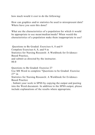
  • 8. severe airfl ow limitation groups signifi cantly different regarding married/cohabitating status? Provide a rationale for your answer. 5. List at least three other relevant demographic variables the researchers might have gathered data on to describe this study sample. 6. For the total sample, what physical symptoms were experienced by ≥ 50% of the subjects? Identify the physical symptoms and the percentages of the total sample experiencing each symptom. Interpreting Line Graphs EXERCISE 7 69 Interpreting Line Graphs STATISTICAL TECHNIQUE IN REVIEW Tables and fi gures are commonly used to present fi ndings from studies or to provide a way for researchers to become familiar with research data. Using fi gures, researchers are able to illustrate the results from descriptive data analyses, assist in identifying patterns in data, identify changes over time, and interpret exploratory fi ndings. A line graph is a fi gure that is developed by joining a series of plotted points with a line to illustrate how a variable changes over time. A line graph fi gure includes a horizontal scale, or x -axis, and a vertical scale, or y -axis. The x -axis is used to document time, and the y -axis is used to document the mean scores or values for a variable ( Grove, Burns, & Gray, 2013 ; Plichta & Kelvin, 2013 ). Researchers might include a line graph to compare the values for three or four variables in a study or to identify the changes in groups for a selected variable over time. For example, Figure 7-1 presents a line graph that documents time in weeks on the x -axis and mean weight loss in pounds on the y -axis for an experimental group consuming a low carbohydrate diet and a control group consuming a standard diet. This line graph illustrates the trend of a strong, steady increase in the mean weight lost by the experimental or intervention group and minimal mean weight loss by the control group. EXERCISE 7
  • 9. FIGURE 7-1 ■ LINE GRAPH COMPARING EXPERIMENTAL AND CONTROL GROUPS FOR WEIGHT LOSS OVER FOUR WEEKS. Weight loss (lbs)Weeksy-axisx- axisControlExperimental10864201234 70EXERCISE 7 • Interpreting Line GraphsCopyright © 2017, Elsevier Inc. All rights reserved. RESEARCH ARTICLE Source Azzolin, K., Mussi, C. M., Ruschel, K. B., de Souza, E. N., Lucena, A. D., & Rabelo-Silva, E. R. (2013). Effectiveness of nursing interventions in heart failure patients in home care using NANDA-I, NIC, and NOC. Applied Nursing Research, 26 (4), 239–244. Introduction Azzolin and colleagues (2013) analyzed data from a larger randomized clinical trial to determine the effectiveness of 11 nursing interventions (NIC) on selected nursing out-comes (NOC) in a sample of patients with heart failure (HF) receiving home care. A total of 23 patients with HF were followed for 6 months after hospital discharge and provided four home visits and four telephone calls. The home visits and phone calls were organized using the nursing diagnoses from the North American Nursing Diagnosis Association International (NANDA-I) classifi cation list. The researchers found that eight nursing interven tions signifi cantly improved the nursing outcomes for these HF patients. Those interventions included “health education, self-modifi cation assistance, behavior modifi -cation, telephone consultation, nutritional counselling, teaching: prescribed medications, teaching: disease process, and energy management” ( Azzolin et al., 2013 , p. 243). The researchers concluded that the NANDA- I, NIC, and NOC linkages were useful in manag-ing patients with HF in their home. Relevant Study Results Azzolin and colleagues (2013) presented their results in a line graph format to display the nursing outcome changes over the 6 months of the home visits and phone calls. The nursing outcomes were measured with a fi ve-point Likert scale with 1 = worst and 5 = best. “Of the eight outcomes selected and measured during the
  • 10. visits, four belonged to the health & knowledge behavior domain (50%), as follows: knowledge: treatment regimen; compliance behavior; knowledge: medication; and symptom control. Signifi cant increases were observed in this domain for all outcomes when comparing mean scores obtained at visits no. 1 and 4 ( Figure 1 ; p < 0.001 for all comparisons). The other four outcomes assessed belong to three different NOC domains, namely, functional health (activity tolerance and energy conservation), physiologic health (fl uid balance), and family health (family participation in professional care). The scores obtained for activity tolerance and energy conservation increased signifi cantly from visit no. 1 to visit no. 4 ( p = 0.004 and p < 0.001, respectively). Fluid balance and family participation in professional care did not show statistically signifi cant differences ( p = 0.848 and p = 0.101, respectively) ( Figure 2 )” ( Azzolin et al., 2013 , p. 241). The signifi cance level or alpha ( α ) was set at 0.05 for this study. Interpreting Line Graphs • EXERCISE 7Copyright © 2017, Elsevier Inc. All rights reserved. FIGURE 2 ■ NURSING OUTCOMES MEASURED OVER 6 MONTHS (OTHER DOMAINS): Activity tolerance (95% CI − 1.38 to − 0.18, p = 0.004); energy conservation (95% CI − 0.62 to − 0.19, p < 0.001); fl uid balance (95% CI − 0.25 to 0.07, p = .848); family participation in professional care (95% CI − 2.31 to − 0.11, p = 0.101). HV = home visit. CI = confi dence interval. Azzolin, K., Mussi, C. M., Ruschel, K. B., de Souza, E. N., Lucena, A. D., & Rabelo-Silva, E. R. (2013). Effectiveness of nursing interventions in heart failure patients in home care using NANDA-I, NIC, and NOC. Applied Nursing Research, 26 (4), p. 242. 5.04.54.03.53.02.52.01.51.00.50MeanHV1HV2HV3HV4Fluid balanceFamily participationin professional careActivity toleranceEnergy conservation FIGURE 1 ■ NURSING OUTCOMES MEASURED OVER 6 MONTHS
  • 11. (HEALTH & KNOWLEDGE BEHAVIOR DOMAIN): Knowledge: medication (95% CI − 1.66 to − 0.87, p < 0.001); knowledge: treatment regimen (95% CI − 1.53 to − 0.98, p < 0.001); symptom control (95% CI − 1.93 to − 0.95, p < 0.001); and compliance behavior (95% CI − 1.24 to − 0.56, p < 0.001). HV = home visit. CI = confi dence interval. 5.04.54.03.53.02.52.01.51.00.50MeanHV1HV2HV3HV4Compli ance behaviorSymptom controlKnowledge: medicationKnowledge: treatment reg 72EXERCISE 7 • Interpreting Line GraphsCopyright © 2017, Elsevier Inc. All rights reserved. STUDY QUESTIONS 1. What is the purpose of a line graph? What elements are included in a line graph? 2. Review Figure 1 and identify the focus of the x -axis and the y - axis. What is the time frame for the x -axis? What variables are presented on this line graph? 3. In Figure 1 , did the nursing outcome compliance behavior change over the 6 months of home visits? Provide a rationale for your answer. 4. State the null hypothesis for the nursing outcome compliance behavior. 5. Was there a signifi cant difference in compliance behavior from the fi rst home visit (HV1) to the fourth home visit (HV4)? Was the null hypothesis accepted or rejected? Provide a rationale for your answer. 6. In Figure 1 , what outcome had the lowest mean at HV1? Did this outcome improve over the four home visits? Provide a rationale for your answer. Copyright © 2017, Elsevier Inc. All rights reserved. 77 Questions to Be Graded EXERCISE 7 Follow your instructor ’ s directions to submit your answers to the following questions for grading. Your instructor may ask you to write your answers below and submit them as a hard copy for grading. Alternatively, your instructor may ask you to use the space below for notes and submit your answers online at http://evolve.elsevier.com/Grove/statistics/ under “Questions to Be Graded.”
  • 12. 1. What is the focus of the example Figure 7-1 in the section introducing the statistical technique of this exercise? 2. In Figure 2 of the Azzolin et al. (2013 , p. 242) study, did the nursing outcome activity tolerance change over the 6 months of home visits (HVs) and telephone calls? Provide a rationale for your answer. 3. State the null hypothesis for the nursing outcome activity tolerance. 4. Was there a signifi cant difference in activity tolerance from the fi rst home visit (HV1) to the fourth home visit (HV4)? Was the null hypothesis accepted or rejected? Provide a rationale for your answer. 5. In Figure 2 , what nursing outcome had the lowest mean at HV1? Did this outcome improve over the four HVs? Provide a rationale for your answer. 6. What nursing outcome had the highest mean at HV1 and at HV4? Was this outcome signifi -cantly different from HV1 to HV4? Provide a rationale for your answer. 7. State the null hypothesis for the nursing outcome family participation in professional care. 8. Was there a statistically signifi cant difference in family participation in professional care from HV1 to HV4? Was the
  • 13. null hypothesis accepted or rejected? Provide a rationale for your answer. 9. Was Figure 2 helpful in understanding the nursing outcomes for patients with heart failure (HF) who received four HVs and telephone calls? Provide a rationale for your answer. 10. What nursing interventions signifi cantly improved the nursing outcomes for these patients with HF? What implications for practice do you note from these study results? Copyright © 2017, Elsevier Inc. All rights reserved. 79 Measures of Central Tendency : Mean, Median, and Mode EXERCISE 8 STATISTICAL TECHNIQUE IN REVIEW Mean, median, and mode are the three measures of central tendency used to describe study variables. These statistical techniques are calculated to determine the center of a distribution of data, and the central tendency that is calculated is determined by the level of measurement of the data (nominal, ordinal, interval, or ratio; see Exercise 1 ). The mode is a category or score that occurs with the greatest frequency in a distribution of scores in a data set. The mode is the only acceptable measure of central tendency for analyzing nominal-level data, which are not continuous and cannot be ranked, compared, or sub-jected to mathematical operations. If a distribution has two scores that occur more fre-quently than others (two modes), the distribution is called bimodal . A distribution with more than two modes is multimodal ( Grove, Burns, & Gray, 2013 ). The median ( MD ) is a score that lies in the middle of a rank-ordered list of values of a distribution. If a distribution consists of an odd number of scores, the MD is the middle score that divides the rest of the distribution into two equal parts, with half of the values falling above the middle score and half of the values falling below this score. In a distribu-tion with an even number of scores, the MD is half of the sum of the two middle numbers of that distribution. If several scores in a distribution are of the same
  • 14. value, then the MD will be the value of the middle score. The MD is the most precise measure of central ten-dency for ordinal-level data and for nonnormally distributed or skewed interval- or ratio-level data. The following formula can be used to calculate a median in a distribution of scores. Median()()MDN=+÷12 N is the number of scores ExampleMedianscoreth:N==+=÷=31311232216 ExampleMedianscoreth:.N==+=÷=404012412205 Thus in the second example, the median is halfway between the 20 th and the 21 st scores. The mean ( X ) is the arithmetic average of all scores of a sample, that is, the sum of its individual scores divided by the total number of scores. The mean is the most accurate measure of central tendency for normally distributed data measured at the interval and ratio levels and is only appropriate for these levels of data (Grove, Gray, & Burns, 2015). In a normal distribution, the mean, median, and mode are essentially equal (see Exercise 26 for determining the normality of a distribution). The mean is sensitive to extreme Copyright © 2017, Elsevier Inc. All rights reserved. 77 Questions to Be Graded EXERCISE 7 Follow your instructor ’ s directions to submit your answers to the following questions for grading. Your instructor may ask you to write your answers below and submit them as a hard copy for grading. Alternatively, your instructor may ask you to use the space below for notes and submit your answers online at http://evolve.elsevier.com/Grove/statistics/ under “Questions to Be Graded.” 1. What is the focus of the example Figure 7-1 in the section introducing the statistical technique of this exercise? 2. In Figure 2 of the Azzolin et al. (2013 , p. 242) study, did the nursing outcome activity tolerance change over the 6 months of home visits (HVs) and telephone calls? Provide a rationale for your answer. 3. State the null hypothesis for the nursing outcome activity tolerance. 4. Was there a signifi cant difference in activity tolerance from the fi rst home visit (HV1) to the fourth home visit (HV4)? Was the null hypothesis
  • 15. accepted or rejected? Provide a rationale for your answer. Name: _____________________________________________________ __ Class: _____________________ Date: _____________________________________________________ ______________________________ 78EXERCISE 7 • Interpreting Line GraphsCopyright © 2017, Elsevier Inc. All rights reserved. 5. In Figure 2 , what nursing outcome had the lowest mean at HV1? Did this outcome improve over the four HVs? Provide a rationale for your answer. 6. What nursing outcome had the highest mean at HV1 and at HV4? Was this outcome signifi -cantly different from HV1 to HV4? Provide a rationale for your answer. 7. State the null hypothesis for the nursing outcome family participation in professional care. 8. Was there a statistically signifi cant difference in family participation in professional care from HV1 to HV4? Was the null hypothesis accepted or rejected? Provide a rationale for your answer. 9. Was Figure 2 helpful in understanding the nursing outcomes for patients with heart failure (HF) who received four HVs and telephone calls? Provide a rationale for your answer. 10. What nursing interventions signifi cantly improved the nursing outcomes for these patients with HF? What implications for practice do you note from these study results? Copyright © 2017, Elsevier Inc. All rights reserved. 79 Measures of Central Tendency : Mean, Median, and Mode EXERCISE 8 STATISTICAL TECHNIQUE IN REVIEW Mean, median, and mode are the three measures of central tendency used to describe study variables. These statistical techniques are calculated to determine the center of a distribution of data, and the central tendency that is calculated is determined by the level of measurement of the data (nominal, ordinal, interval, or ratio; see Exercise 1 ). The mode is a category or score that occurs with the greatest frequency in a distribution of scores in a data set. The mode is the only acceptable measure of central tendency for analyzing nominal-level data, which are not continuous and cannot be ranked, compared, or sub-jected to
  • 16. mathematical operations. If a distribution has two scores that occur more fre-quently than others (two modes), the distribution is called bimodal . A distribution with more than two modes is multimodal ( Grove, Burns, & Gray, 2013 ). The median ( MD ) is a score that lies in the middle of a rank-ordered list of values of a distribution. If a distribution consists of an odd number of scores, the MD is the middle score that divides the rest of the distribution into two equal parts, with half of the values falling above the middle score and half of the values falling below this score. In a distribu-tion with an even number of scores, the MD is half of the sum of the two middle numbers of that distribution. If several scores in a distribution are of the same value, then the MD will be the value of the middle score. The MD is the most precise measure of central ten-dency for ordinal-level data and for nonnormally distributed or skewed interval- or ratio-level data. The following formula can be used to calculate a median in a distribution of scores. Median()()MDN=+÷12 N is the number of scores ExampleMedianscoreth:N==+=÷=31311232216 ExampleMedianscoreth:.N==+=÷=404012412205 Thus in the second example, the median is halfway between the 20 th and the 21 st scores. The mean ( X ) is the arithmetic average of all scores of a sample, that is, the sum of its individual scores divided by the total number of scores. The mean is the most accurate measure of central tendency for normally distributed data measured at the interval and ratio levels and is only appropriate for these levels of data (Grove, Gray, & Burns, 2015). In a normal distribution, the mean, median, and mode are essentially equal (see Exercise 26 for determining the normality of a distribution). The mean is sensitive to extreme Copyright © 2017, Elsevier Inc. All rights reserved. 77 Questions to Be Graded EXERCISE 7 Follow your instructor ’ s directions to submit your answers to the following questions for
  • 17. grading. Your instructor may ask you to write your answers below and submit them as a hard copy for grading. Alternatively, your instructor may ask you to use the space below for notes and submit your answers online at http://evolve.elsevier.com/Grove/statistics/ under “Questions to Be Graded.” 1. What is the focus of the example Figure 7-1 in the section introducing the statistical technique of this exercise? 2. In Figure 2 of the Azzolin et al. (2013 , p. 242) study, did the nursing outcome activity tolerance change over the 6 months of home visits (HVs) and telephone calls? Provide a rationale for your answer. 3. State the null hypothesis for the nursing outcome activity tolerance. 4. Was there a signifi cant difference in activity tolerance from the fi rst home visit (HV1) to the fourth home visit (HV4)? Was the null hypothesis accepted or rejected? Provide a rationale for your answer. 5. In Figure 2 , what nursing outcome had the lowest mean at HV1? Did this outcome improve over the four HVs? Provide a rationale for your answer. 6. What nursing outcome had the highest mean at HV1 and at HV4? Was this outcome signifi -cantly different from HV1 to HV4? Provide a rationale for your answer. 7. State the null hypothesis for the nursing outcome family participation in professional care.
  • 18. 8. Was there a statistically signifi cant difference in family participation in professional care from HV1 to HV4? Was the null hypothesis accepted or rejected? Provide a rationale for your answer. 9. Was Figure 2 helpful in understanding the nursing outcomes for patients with heart failure (HF) who received four HVs and telephone calls? Provide a rationale for your answer. 10. What nursing interventions signifi cantly improved the nursing outcomes for these patients with HF? What implications for practice do you note from these study results? Copyright © 2017, Elsevier Inc. All rights reserved. 79 Measures of Central Tendency : Mean, Median, and Mode EXERCISE 8 STATISTICAL TECHNIQUE IN REVIEW Mean, median, and mode are the three measures of central tendency used to describe study variables. These statistical techniques are calculated to determine the center of a distribution of data, and the central tendency that is calculated is determined by the level of measurement of the data (nominal, ordinal, interval, or ratio; see Exercise 1 ). The mode is a category or score that occurs with the greatest frequency in a distribution of scores in a data set. The mode is the only acceptable measure of central tendency for analyzing nominal-level data, which are not continuous and cannot be ranked, compared, or sub-jected to mathematical operations. If a distribution has two scores that occur more fre-quently than others (two modes), the distribution is called bimodal . A distribution with more than two modes is multimodal ( Grove, Burns, & Gray, 2013 ). The median ( MD ) is a score that lies in the middle of a rank-ordered list of values of a distribution. If a distribution consists of an odd number of scores, the MD is the middle score that divides the rest of the distribution into two equal parts, with half of the values falling
  • 19. above the middle score and half of the values falling below this score. In a distribu-tion with an even number of scores, the MD is half of the sum of the two middle numbers of that distribution. If several scores in a distribution are of the same value, then the MD will be the value of the middle score. The MD is the most precise measure of central ten-dency for ordinal-level data and for nonnormally distributed or skewed interval- or ratio-level data. The following formula can be used to calculate a median in a distribution of scores. Median()()MDN=+÷12 N is the number of scores ExampleMedianscoreth:N==+=÷=31311232216 ExampleMedianscoreth:.N==+=÷=404012412205 Thus in the second example, the median is halfway between the 20 th and the 21 st scores. The mean ( X ) is the arithmetic average of all scores of a sample, that is, the sum of its individual scores divided by the total number of scores. The mean is the most accurate measure of central tendency for normally distributed data measured at the interval and ratio levels and is only appropriate for these levels of data (Grove, Gray, & Burns, 2015). In a normal distribution, the mean, median, and mode are essentially equal (see Exercise 26 for determining the normality of a distribution). The mean is sensitive to extreme Copyright © 2017, Elsevier Inc. All rights reserved. 291 Calculating Descriptive Statistics There are two major classes of statistics: descriptive statistics and inferential statistics. Descriptive statistics are computed to reveal characteristics of the sample data set and to describe
  • 20. study variables. Inferential statistics are computed to gain information about effects and associations in the population being studied. For some types of studies, descriptive statistics will be the only approach to analysis of the data. For other studies, descriptive statistics are the fi rst step in the data analysis process, to be followed by infer-ential statistics. For all studies that involve numerical data, descriptive statistics are crucial in understanding the fundamental properties of the variables being studied. Exer-cise 27 focuses only on descriptive statistics and will illustrate the most common descrip-tive statistics computed in nursing research and provide examples using actual clinical data from empirical publications. MEASURES OF CENTRAL TENDENCY A measure of central tendency is a statistic that represents the center or middle of a frequency distribution. The three measures of central tendency commonly used in nursing research are the mode, median ( MD ), and mean ( X ). The mean is the arithmetic average of all of a variable ’ s values. The median is the exact middle value (or the average of the middle two values if there is an even number of observations). The mode is the most commonly occurring value or values (see Exercise 8 ). The following data have been collected from veterans with rheumatoid arthritis ( Tran, Hooker, Cipher, & Reimold, 2009 ). The values in Table 27-1 were extracted from a larger sample of veterans who had a history of biologic medication use (e.g., infl iximab [Remi- cade], etanercept [Enbrel]). Table 27-1 contains data collected from 10 veterans who had stopped taking biologic medications, and the variable represents the number of years that each veteran had taken the medication before stopping. Because the number of study subjects represented below is 10, the correct statistical notation to refl ect that number is: n=10 Note that the n is lowercase, because we are referring to a sample of veterans. If the data being presented represented the entire population of veterans, the correct notation is the uppercase N. Because most nursing research is conducted using samples, not popu-lations, all formulas in the subsequent exercises will incorporate the
  • 21. sample notation, n. Mode The mode is the numerical value or score that occurs with the greatest frequency; it does not necessarily indicate the center of the data set. The data in Table 27-1 contain two EXERCISE 27 292EXERCISE 27 • Calculating Descriptive StatisticsCopyright © 2017, Elsevier Inc. All rights reserved. modes: 1.5 and 3.0. Each of these numbers occurred twice in the data set. When two modes exist, the data set is referred to as bimodal ; a data set that contains more than two modes would be multimodal . Median The median ( MD ) is the score at the exact center of the ungrouped frequency distribution. It is the 50th percentile. To obtain the MD , sort the values from lowest to highest. If the number of values is an uneven number, exactly 50% of the values are above the MD and 50% are below it. If the number of values is an even number, the MD is the average of the two middle values. Thus the MD may not be an actual value in the data set. For example, the data in Table 27-1 consist of 10 observations, and therefore the MD is calculated as the average of the two middle values. MD=+()=15202175... Mean The most commonly reported measure of central tendency is the mean. The mean is the sum of the scores divided by the number of scores being summed. Thus like the MD, the mean may not be a member of the data set. The formula for calculating the mean is as follows: XXn=∑ where X = mean ∑ = sigma, the statistical symbol for summation X = a single value in the sample n = total number of values in the sample The mean number of years that the veterans used a biologic medication is calculated as follows: X=+++++++++()=010313151520223030401019...........years TABLE 27-1 DURATION OF BIOLOGIC USE AMONG VETERANS WITH RHEUMATOID ARTHRITIS ( n = 10) Duration of Biologic Use (years) 0.10.31.31.51.52.02.23.03.04.0 293Calculating Descriptive Statistics • EXERCISE 27Copyright © 2017, Elsevier Inc. All rights reserved. The mean is an appropriate measure of central tendency for approximately normally distributed populations with variables measured at the interval or ratio level. It is also
  • 22. appropriate for ordinal level data such as Likert scale values, where higher numbers rep-resent more of the construct being measured and lower numbers represent less of the construct (such as pain levels, patient satisfaction, depression, and health status). The mean is sensitive to extreme scores such as outliers. An outlier is a value in a sample data set that is unusually low or unusually high in the context of the rest of the sample data. An example of an outlier in the data presented in Table 27-1 might be a value such as 11. The existing values range from 0.1 to 4.0, meaning that no veteran used a biologic beyond 4 years. If an additional veteran were added to the sample and that person used a biologic for 11 years, the mean would be much larger: 2.7 years. Simply adding this outlier to the sample nearly doubled the mean value. The outlier would also change the frequency distribution. Without the outlier, the frequency distribution is approximately normal, as shown in Figure 27-1 . Including the outlier changes the shape of the distribution to appear positively skewed. Although the use of summary statistics has been the traditional approach to describing data or describing the characteristics of the sample before inferential statistical analysis, its ability to clarify the nature of data is limited. For example, using measures of central tendency, particularly the mean, to describe the nature of the data obscures the impact of extreme values or deviations in the data. Thus, signifi cant features in the data may be concealed or misrepresented. Often, anomalous, unexpected, or problematic data and discrepant patterns are evident, but are not regarded as meaningful. Measures of disper-sion, such as the range, difference scores, variance, and standard deviation ( SD ), provide important insight into the nature of the data. MEASURES OF DISPERSION Measures of dispersion , or variability, are measures of individual differences of the members of the population and sample. They indicate how values in a sample are dis-persed around the mean. These measures provide information about the data that is not available from measures of central tendency. They indicate how
  • 23. different the scores are—the extent to which individual values deviate from one another. If the individual values are similar, measures of variability are small and the sample is relatively homogeneous in terms of those values. Heterogeneity (wide variation in scores) is important in some statistical procedures, such as correlation. Heterogeneity is determined by measures of variability. The measures most commonly used are range, difference scores, variance, and SD (see Exercise 9 ). FIGURE 27-1 ■ FREQUENCY DISTRIBUTION OF YEARS OF BIOLOGIC USE, WITHOUT OUTLIER AND WITH OUTLIER. 0FrequencyFrequency3-3.90-0.92-2.91-1.94-4.93-3.90-.91-1.92- 2.94-4.95-5.96-6.97-7.98-8.99-9.910-10.911-11.9Years of biologic useYears of biologic use3.02.52.01.51.00.503.02.52.01.51.00.5 294EXERCISE 27 • Calculating Descriptive StatisticsCopyright © 2017, Elsevier Inc. All rights reserved. Range The simplest measure of dispersion is the range . In published studies, range is presented in two ways: (1) the range is the lowest and highest scores, or (2) the range is calculated by subtracting the lowest score from the highest score. The range for the scores in Table 27-1 is 0.3 and 4.0, or it can be calculated as follows: 4.0 − 0.3 = 3.7. In this form, the range is a difference score that uses only the two extreme scores for the comparison. The range is generally reported but is not used in further analyses. Difference Scores Difference scores are obtained by subtracting the mean from each score. Sometimes a difference score is referred to as a deviation score because it indicates the extent to which a score deviates from the mean. Of course, most variables in nursing research are not “scores,” yet the term difference score is used to represent a value ’ s deviation from the mean. The difference score is positive when the score is above the mean, and it is negative when the score is below the mean (see Table 27-2 ). Difference scores are the basis for many statistical analyses and can be found within many statistical equations. The formula for
  • 24. difference scores is: XX− Σof absolute values95:. TABLE 27-2 DIFFERENCE SCORES OF DURATION OF BIOLOGIC USE X --X XX-- 0.1 − 1.9 − 1.80.3 − 1.9 − 1.61.3 − 1.9 − 0.61.5 − 1.9 − 0.41.5 − 1.9 − 0.42.0 − 1.90.12.2 − 1.90.33.0 − 1.91.13.0 − 1.91.14.0 − 1.92.1 The mean deviation is the average difference score, using the absolute values. The formula for the mean deviation is: XXXndeviation=−∑ In this example, the mean deviation is 0.95. This value was calculated by taking the sum of the absolute value of each difference score (1.8, 1.6, 0.6, 0.4, 0.4, 0.1, 0.3, 1.1, 1.1, 2.1) and dividing by 10. The result indicates that, on average, subjects ’ duration of biologic use deviated from the mean by 0.95 years. Variance Variance is another measure commonly used in statistical analysis. The equation for a sample variance ( s 2 ) is below. sXXn221=−()−∑ 295Calculating Descriptive Statistics • EXERCISE 27Copyright © 2017, Elsevier Inc. All rights reserved. Note that the lowercase letter s 2 is used to represent a sample variance. The lowercase Greek sigma ( σ 2 ) is used to represent a population variance, in which the denominator is N instead of n − 1. Because most nursing research is conducted using samples, not popu-lations, formulas in the subsequent exercises that contain a variance or standard deviation will incorporate the sample notation, using n − 1 as the denominator. Moreover, statistical software packages compute the variance and standard deviation using the sample formu-las, not the population formulas. The variance is always a positive value and has no upper limit. In general, the larger the variance, the larger the dispersion of scores. The variance is most often computed to derive the standard deviation because, unlike the variance, the standard deviation refl ects impor-tant properties about the frequency distribution of the variable it represents. Table 27-3 displays how we would compute a variance by hand, using the biologic duration data. s213419=. s²=1.49 TABLE 27-3 VARIANCE COMPUTATION OF BIOLOGIC USE X X XX-- XX--(())2 0.1 − 1.9 − 1.83.240.3 − 1.9 − 1.62.561.3 − 1.9 − 0.60.361.5 − 1.9 − 0.40.161.5 − 1.9 − 0.40.162.0 − 1.90.10.012.2 − 1.90.30.093.0 −
  • 25. 1.91.11.213.0 − 1.91.11.214.0 − 1.92.14.41 Σ 13.41 Standard Deviation Standard deviation is a measure of dispersion that is the square root of the variance. The standard deviation is represented by the notation s or SD . The equation for obtaining a standard deviation is SDX=−()−∑Xn21 Table 27-3 displays the computations for the variance. To compute the SD , simply take the square root of the variance. We know that the variance of biologic duration is s 2 = 1.49. Therefore, the s of biologic duration is SD = 1.22. The SD is an important sta-tistic, both for understanding dispersion within a distribution and for interpreting the relationship of a particular value to the distribution. SAMPLING ERROR A standard error describes the extent of sampling error. For example, a standard error of the mean is calculated to determine the magnitude of the variability associated with the mean. A small standard error is an indication that the sample mean is close to 296EXERCISE 27 • Calculating Descriptive StatisticsCopyright © 2017, Elsevier Inc. All rights reserved. the population mean, while a large standard error yields less certainty that the sample mean approximates the population mean. The formula for the standard error of the mean ( sX ) is: ssnX= Using the biologic medication duration data, we know that the standard deviation of biologic duration is s = 1.22. Therefore, the standard error of the mean for biologic dura-tion is computed as follows: sX=12210. sX=039. The standard error of the mean for biologic duration is 0.39. Confi dence Intervals To determine how closely the sample mean approximates the population mean, the stan-dard error of the mean is used to build a confi dence interval. For that matter, a confi dence interval can be created for many statistics, such as a mean, proportion, and odds ratio. To build a confi dence interval around a statistic, you must have the standard error value and the t value to adjust the standard error. The degrees of freedom ( df ) to use to compute a confi dence interval is df = n − 1. To compute the confi dence interval for a mean, the lower and upper limits of that interval are created by multiplying the sX by the t statistic, where df = n − 1. For a
  • 26. 95% confi dence interval, the t value should be selected at α = 0.05. For a 99% confi dence inter-val, the t value should be selected at α = 0.01. Using the biologic medication duration data, we know that the standard error of the mean duration of biologic medication use is sX=039. . The mean duration of biologic medication use is 1.89. Therefore, the 95% confi dence interval for the mean duration of biologic medication use is computed as follows: XstX± 189039226...±()() 189088..± As referenced in Appendix A , the t value required for the 95% confi dence interval with df = 9 is 2.26. The computation above results in a lower limit of 1.01 and an upper limit of 2.77. This means that our confi dence interval of 1.01 to 2.77 estimates the population mean duration of biologic use with 95% confi dence ( Kline, 2004 ). Technically and math-ematically, it means that if we computed the mean duration of biologic medication use on an infi nite number of veterans, exactly 95% of the intervals would contain the true population mean, and 5% would not contain the population mean ( Gliner, Morgan, & Leech, 2009 ). If we were to compute a 99% confi dence interval, we would require the t value that is referenced at α = 0.01. Therefore, the 99% confi dence interval for the mean duration of biologic medication use is computed as follows: 189039325...±()() 189127..± 297Calculating Descriptive Statistics • EXERCISE 27Copyright © 2017, Elsevier Inc. All rights reserved. As referenced in Appendix A , the t value required for the 99% confi dence interval with df = 9 is 3.25. The computation above results in a lower limit of 0.62 and an upper limit of 3.16. This means that our confi dence interval of 0.62 to 3.16 estimates the population mean duration of biologic use with 99% confi dence. Degrees of Freedom The concept of degrees of freedom ( df ) was used in reference to computing a confi dence interval. For any statistical computation, degrees of freedom are the number of inde-pendent pieces of information that are free to vary in order to estimate another piece of information ( Zar, 2010 ). In the case of the confi dence interval, the degrees of freedom are n − 1. This means that there are n − 1 independent observations
  • 27. in the sample that are free to vary (to be any value) to estimate the lower and upper limits of the confi dence interval. SPSS COMPUTATIONS A retrospective descriptive study examined the duration of biologic use from veterans with rheumatoid arthritis ( Tran et al., 2009 ). The values in Table 27-4 were extracted from a larger sample of veterans who had a history of biologic medication use (e.g., infl iximab [Remicade], etanercept [Enbrel]). Table 27-4 contains simulated demographic data col-lected from 10 veterans who had stopped taking biologic medications. Age at study enroll-ment, duration of biologic use, race/ethnicity, gender (F = female), tobacco use (F = former use, C = current use, N = never used), primary diagnosis (3 = irritable bowel syndrome, 4 = psoriatic arthritis, 5 = rheumatoid arthritis, 6 = reactive arthritis), and type of biologic medication used were among the study variables examined. TABLE 27-4 DEMOGRAPHIC VARIABLES OF VETERANS WITH RHEUMATOID ARTHRITIS Patient ID Duration (yrs) Age Race/Ethnicity Gender Tobacco Diagnosis Biologic 10.142CaucasianFF5Infl iximab20.341Black, not of Hispanic OriginFF5Etanercept31.356CaucasianFN5Infl iximab41.578CaucasianFF3Infl iximab51.586Black, not of Hispanic OriginFF4Etanercept62.049CaucasianFF6Etanercept72.282Cauc asianFF5Infl iximab83.035CaucasianFN3Infl iximab93.059Black, not of Hispanic OriginFC3Infl iximab104.037CaucasianFF5Etanercept 298EXERCISE 27 • Calculating Descriptive StatisticsCopyright © 2017, Elsevier Inc. All rights reserved. This is how our data set looks in SPSS. Step 1: For a nominal variable, the appropriate descriptive statistics are frequencies and percentages. From the “Analyze” menu, choose “Descriptive Statistics” and “Frequen-cies.” Move “Race/Ethnicity and Gender” over to the right. Click “OK.” 299Calculating Descriptive Statistics • EXERCISE 27Copyright © 2017, Elsevier Inc. All rights reserved. Step 2: For a continuous variable, the appropriate descriptive statistics are means and standard deviations. From the “Analyze” menu,
  • 28. choose “Descriptive Statistics” and “Explore.” Move “Duration” over to the right. Click “OK.” INTERPRETATION OF SPSS OUTPUT The following tables are generated from SPSS. The fi rst set of tables (from the fi rst set of SPSS commands in Step 1) contains the frequencies of race/ethnicity and gender. Most (70%) were Caucasian, and 100% were female. Frequencies Frequency Table RaceEthnicityFrequencyPercentValid PercentCumulative PercentValidBlack, not of Hispanic Origin330.030.030.0Caucasian770.070.0100.0Total10100.0100. 0GenderFrequencyPercentValid PercentCumulative PercentValidF10100.0100.0100.0 300EXERCISE 27 • Calculating Descriptive StatisticsCopyright © 2017, Elsevier Inc. All rights reserved. DescriptivesStatisticStd. ErrorDuration of Biologic Use1.890.3860Lower Bound1.017Upper Bound2.7631.8721.7501.4901.2206.14.03.92.0.159.687- .4371.334Mean95% Confidence Interval for Mean 5% Trimmed MeanMedianVarianceStd. DeviationMinimumMaximumRangeInterquartile RangeSkewnessKurtosis The second set of output (from the second set of SPSS commands in Step 2) contains the descriptive statistics for “Duration,” including the mean, s (standard deviation), SE , 95% confi dence interval for the mean, median, variance, minimum value, maximum value, range, and skewness and kurtosis statistics. As shown in the output, mean number of years for duration is 1.89, and the SD is 1.22. The 95% CI is 1.02–2.76. Explore 301Calculating Descriptive Statistics • EXERCISE 27Copyright © 2017, Elsevier Inc. All rights reserved. STUDY QUESTIONS 1. Defi ne mean. 2. What does this symbol, s 2 , represent? 3. Defi ne outlier. 4. Are there any outliers among the values representing duration of biologic use? 5. How would you interpret the 95% confi dence interval for the mean of duration of biologic use? 6. What percentage of patients were Black, not of Hispanic origin? 7. Can you compute the variance for duration of biologic use by using the information presented in the SPSS output above?
  • 29. Copyright © 2017, Elsevier Inc. All rights reserved. 305 Questions to Be Graded EXERCISE 27 Follow your instructor ’ s directions to submit your answers to the following questions for grading. Your instructor may ask you to write your answers below and submit them as a hard copy for grading. Alternatively, your instructor may ask you to use the space below for notes and submit your answers online at http://evolve.elsevier.com/Grove/statistics/ under “ Name: _____________________________________________________ __ Class: _____________________ Date:_____________________ Questions to Be Graded.” 1. What is the mean age of the sample data? 2. What percentage of patients never used tobacco? 3. What is the standard deviation for age? 4. Are there outliers among the values of age? Provide a rationale for your answer.
  • 30. 5. What is the range of age values? 6. What percentage of patients were taking infl iximab? 7. What percentage of patients had rheumatoid arthritis as their primary diagnosis? 8. What percentage of patients had irritable bowel syndrome as their primary diagnosis? 9. What is the 95% CI for age? 10. What percentage of patients had psoriatic arthritis as their primary diagnosis? Copyright © 2017, Elsevier Inc. All rights reserved. 307 Calculating Pearson Product-Moment Correlation Coeffi cient Correlational analyses identify associations between two variables. There are many differ-ent kinds of statistics that yield a measure of correlation. All of these statistics address a research question or hypothesis that involves an association or relationship. Examples of research questions that are answered with correlation statistics are, “Is there an associa-tion between weight loss and depression?” and “Is there a relationship between patient satisfaction and health status?” A hypothesis is developed to identify the nature (positive or negative) of the
  • 31. relationship between the variables being studied. The Pearson product-moment correlation was the fi rst of the correlation measures developed and is the most commonly used. As is explained in Exercise 13 , this coeffi cient (statistic) is represented by the letter r , and the value of r is always between − 1.00 and + 1.00. A value of zero indicates no relationship between the two variables. A positive cor-relation indicates that higher values of x are associated with higher values of y . A negative or inverse correlation indicates that higher values of x are associated with lower values of y . The r value is indicative of the slope of the line (called a regression line) that can be drawn through a standard scatterplot of the two variables (see Exercise 11 ). The strengths of different relationships are identifi ed in Table 28-1 ( Cohen, 1988 ). EXERCISE 28 TABLE 28-1 STRENGTH OF ASSOCIATION FOR PEARSON r Strength of Association Positive Association Negative Association Weak association0.00 to < 0.300.00 to < − 0.30Moderate association0.30 to 0.49 − 0.49 to − 0.30Strong association0.50 or greater − 1.00 to − 0.50 RESEARCH DESIGNS APPROPRIATE FOR THE PEARSON r Research designs that may utilize the Pearson r include any associational design ( Gliner, Morgan, & Leech, 2009 ). The variables involved in the design are attributional, meaning the variables are characteristics of the participant, such as health status, blood pressure, gender, diagnosis, or ethnicity. Regardless of the nature of variables, the variables submit-ted to a Pearson correlation must be measured as continuous or at the interval or ratio level. STATISTICAL FORMULA AND ASSUMPTIONS Use of the Pearson correlation involves the following assumptions: 1. Interval or ratio measurement of both variables (e.g., age, income, blood pressure, cholesterol levels). However, if the variables are measured with a Likert scale, and the frequency distribution is approximately normally distributed, these data are