2. standard spectra allows users to evaluate spectral differences
relative to the spectra specified here.
2. Referenced Documents
2.1 ASTM Standards:
E 490 Solar Constant and Air Mass Zero Solar Spectral
Irradiance Tables3
E 772 Terminology Relating to Solar Energy Conversion4
G 113 Terminology Relating to Natural and Artificial
Weathering Tests of Nonmetallic Materials5
3. Terminology
3.1 Definitions—Definitions of most terms used in this
specification may be found in Terminology E 772.
3.2 The following definition differs from that in Terminol-
ogy E 772, representing information current as of this revision.
3.2.1 solar constant—the total solar irradiance at normal
incidence on a surface in free space at the earth’s mean
distance from the sun. (1 astronomical unit, or AU = 1.496 3
1011
m).
3.2.1.1 Discussion—The solar constant is now known
within about 61.5 W·m-2
. Its current accepted values are
1366.1 W·m-2
(ASTM E 490) or 1367.0 W·m-2
(World Meteo-
rological Organization, WMO), and are subject to change. Due
to the eccentricity of the earth’s orbit, the actual extraterrestrial
solar irradiance varies by 63.4 % about the solar constant as
the earth-sun distance varies through the year. Throughout this
standard the solar constant is defined as 1367.0 W·m-2
.
3.3 Definitions of Terms Specific to This Standard:
3.3.1 aerosol optical depth (AOD)—the wavelength-
dependent total extinction (scattering and absorption) by aero-
sols in the atmosphere. This optical depth (also called “optical
thickness”) is defined here at 500 nm.
3.3.1.1 Discussion—See Appendix X1.
3.3.2 air mass zero (AM0)—describes solar radiation quan-
tities outside the Earth’s atmosphere at the mean Earth-Sun
distance (1 Astronomical Unit). See ASTM E 490.
3.3.3 integrated irradiance El1-l2—spectral irradiance inte-
grated over a specific wavelength interval from l1 to l2,
measured in W·m-2
; mathematically:
El12l2 5 *l1
l2
El dl (1)
3.3.4 solar irradiance, hemispherical EH—on a given plane,
the solar radiant flux received from within the 2p steradian
field of view of a tilted plane from the portion of the sky dome
and the foreground included in the plane’s field of view,
including both diffuse and direct solar radiation.
3.3.4.1 Discussion—For the special condition of a horizon-
tal plane the hemispherical solar irradiance is properly termed
global solar irradiance, EG. Incorrectly, global tilted, or total
global irradiance is often used to indicate hemispherical
irradiance for a tilted plane. In case of a sun-tracking receiver,
this hemispherical irradiance is commonly called global nor-
mal irradiance. The adjective global should refer only to
hemispherical solar radiation on a horizontal, not a tilted,
surface.
3.3.5 solar irradiance, spectral El—solar irradiance E per
unit wavelength interval at a given wavelength l (unit: Watts
per square meter per nanometer, W·m-2
·nm-1
):
El 5
dE
dl (2)
3.3.6 spectral interval—the distance in wavelength units
between adjacent spectral irradiance data points.
3.3.7 spectral passband—the effective wavelength interval
within which spectral irradiance is allowed to pass, as through
a filter or monochromator. The convolution integral of the
spectral passband (normalized to unity at maximum) and the
incident spectral irradiance produces the effective transmitted
irradiance.
3.3.7.1 Discussion—Spectral passband may also be referred
to as the spectral bandwidth of a filter or device. Passbands are
usually specified as the interval between wavelengths at which
one half of the maximum transmission of the filter or device
occurs, or as full-width at half-maximum, FWHM.
3.3.8 spectral resolution—the minimum wavelength differ-
ence between two wavelengths that can be identified unam-
biguously.
3.3.8.1 Discussion—In the context of this standard, the
spectral resolution is simply the interval, Dl, between spectral
data points, or the spectral interval.
3.3.9 total ozone—the depth of a column of pure ozone
equivalent to the total of the ozone in a vertical column from
the ground to the top of the atmosphere (unit: atmosphere-cm
or atm-cm).
3.3.10 total precipitable water—the depth of a column of
water (with a section of 1 cm2
) equivalent to the condensed
water vapor in a vertical column from the ground to the top of
the atmosphere (unit: cm or g/cm2
).
3.3.11 wavenumber—a unit of frequency, n, in units of
reciprocal centimeters (symbol cm-1
) commonly used in place
of wavelength, l (units of length, typically nanometers). To
convert wavenumber to nanometers, l nm = 1 · 107
/ n cm-1
.
See X1.2.
4. Significance and Use
4.1 Absorptance, reflectance, and transmittance of solar
energy are important factors in material degradation studies,
solar thermal system performance, solar photovoltaic system
performance, biological studies, and solar simulation activities.
These optical properties are normally functions of wavelength,
which require the spectral distribution of the solar flux be
known before the solar-weighted property can be calculated.
To compare the relative performance of competitive products,
or to compare the performance of products before and after
being subjected to weathering or other exposure conditions, a
reference standard solar spectral distribution is desirable.
4.2 These tables provide appropriate standard spectral irra-
diance distributions for determining the relative optical perfor-
mance of materials, solar thermal, solar photovoltaic, and other
systems. The tables may be used to evaluate components and
materials for the purpose of solar simulation where either the
3
Annual Book of ASTM Standards, Vol 15.03.
4
Annual Book of ASTM Standards, Vol 12.02.
5
National Renewable Energy Lab., 1617 Cole Blvd., MS-3411, Golden, CO
80401.
G 173 – 03
2
3. direct or the hemispherical (that is, direct beam plus diffuse
sky) spectral solar irradiance is desired. However, these tables
are not intended to be used as a benchmark for ultraviolet
radiation used in indoor exposure testing of materials using
manufactured light sources.
4.3 The total integrated irradiances for the direct and hemi-
spherical tilted spectra are 900.1 W·m-2
and 1000.4 W·m-2
,
respectively. Note that, in PV applications, no amplitude
adjustments are required to match standard reporting condition
irradiances of 1000 W·m-2
for hemispherical irradiance.
4.4 Previously defined global hemispherical reference spec-
trum (G 159) for a sun-facing 37°-tilted surface served well to
meet the needs of the flat plate photovoltaic research, devel-
opment, and industrial community. Investigation of prevailing
conditions and measured spectra shows that this global hemi-
spherical reference spectrum can be attained in practice under
a variety of conditions, and that these conditions can be
interpreted as representative for many combinations of atmo-
spheric parameters. Earlier global hemispherical reference
spectrum may be closely, but not exactly, reproduced with
improved spectral wavelength range, uniform spectral interval,
and spectral resolution equivalent to the spectral interval, using
inputs in X1.4.
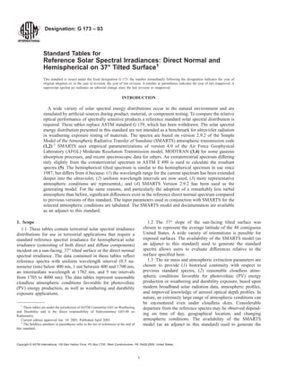
4.5 Reference spectra generated by the SMARTS Version
2.9.2 model for the indicated conditions are shown in Fig. 1.
The exact input file structure required to generate the reference
spectra is shown in Table 1.
4.6 The availability of the adjunct standard computer soft-
ware for SMARTS allows one to (1) reproduce the reference
spectra, using the above input parameters; (2) compute test
spectra to attempt to match measured data at a specified
FWHM, and evaluate atmospheric conditions; and (3) compute
test spectra representing specific conditions for analysis vis-à-
vis any one or all of the reference spectra.
4.7 Differences from the previous standard spectra (G 159)
can be summarized as follows:
4.7.1 Extended spectral interval in the ultraviolet (down to
280 nm, rather than 305 nm),
4.7.2 Better resolution (2002 wavelengths, as compared to
120),
4.7.3 Constant intervals (0.5 nm below 400 nm, 1 nm
between 400 and 1700 nm, and 5 nm above),
4.7.4 Better definition of atmospheric scattering and gas-
eous absorption, with more species considered,
4.7.5 Better defined extraterrestrial spectrum,
4.7.6 More realistic spectral ground reflectance, and
4.7.7 Lower aerosol optical depth, yielding significantly
larger direct normal irradiance.
5. Technical Bases for the Tables
5.1 These tables are modeled data generated using an air
mass zero (AM0) spectrum based in part on the extraterrestrial
spectrum of Kurucz (5), the 1976 U.S. Standard Atmosphere
(6), the Shettle and Fenn Rural Aerosol Profile (7), the
SMARTS radiative transfer code, version 2.9.2, and associated
input data files.
5.2 In order to provide spectral data with a uniform spectral
step size and improved spectral resolution, the AM0 spectrum
FIG. 1 Plot of Direct Normal Spectral Irradiance (Solid Line) and Hemispherical Spectral Irradiance on 37° Tilted Sun-Facing Surface
(Dotted Line) Computed Using Smarts Version 2.9.2 Model With Input File in Table 1
G 173 – 03
3
4. used in conjunction with SMARTS to generate the terrestrial
spectrum is slightly different from the ASTM extraterrestrial
spectrum, ASTM E 490. Because ASTM E 490 and SMARTS
both use the Kurucz data, the SMARTS and E 490 spectra are
in good agreement though they do not have the same spectral
interval step sizes, spectral interval centers, or spectral resolu-
tion.
5.3 The 1976 U.S. Standard Atmosphere (USSA) is used to
provide documented atmospheric properties and concentra-
tions of absorbers. However, some newly documented (and
relatively minor) absorbers are taken into consideration in the
present standard spectra. See X1.3.
5.4 The SMARTS model code and documentation is avail-
able from the NREL (National Renewable Energy Lab) website
(www.nrel.gov).
5.5 These terrestrial solar spectral data are based on the
work of Gueymard (1,2) and Gueymard et al. (8). Previously
defined reference spectra were based on the work of Bird,
Hulstrom, and Lewis (9). The current spectra reflect current (as
of 2002) improved knowledge of gaseous absorption, atmo-
spheric aerosol optical properties, transmission properties, and
radiative transfer modeling.
5.6 The terrestrial solar spectra in the tables have been
computed with a spectral resolution equivalent to that of the
wavelength interval. Parameterizations in the SMARTS2
model are based on high resolution (2 cm-1
) MODTRAN
(2,3,10,11) results subsequently “degraded” or smoothed to the
SMARTS2 model wavelength interval.
5.6.1 Discussion—This approach emulates the procedure of
measuring spectral data with a monochromator by using the
wavelength interval equivalent to the spectral passband of the
instrument.
5.7 To represent favorable conditions for PV energy pro-
duction and exposure conditions for weathering and durability
testing, sites in the National Solar Radiation Data Base (13)
with annual daily average direct normal solar radiation exceed-
ing 6 kWh·m-2
(or 21.6 MJ·m-2
) per day were analyzed. The
mean aerosol optical depth at 500 nm for these sites was
determined to be 0.085. A very slightly smaller AOD of 0.084
results in a hemispherical tilted spectrum integrating to 1000.4
W/m2
, nearly exactly the irradiance used in photovoltaic
standard reporting conditions. See X1.2.
5.8 Previous reference spectra were generated using a
wavelength-independent albedo of 0.2. The present standards
utilize measured wavelength-dependent reflectance data, rep-
resenting light sandy soil of the southwest U.S. See Fig. X1.1.
5.9 The direct normal spectrum includes the circumsolar
spectral irradiance that would be measured with a collimated
spectroradiometer or pyrheliometer with a 5.8° field of view
(aperture half-angle of 2.9°) representing common commer-
cially available radiometers.
TABLE 1 SMARTS Version 2.9.2 Input File to Generate the Reference Spectra
Card ID Value Parameter/Description/Variable Name
1 ’ASTM_G 173_Std_Spectra’ Header
2 1 Pressure input mode (1 = pressure and altitude): ISPR
2a 1013.25 0. Station Pressure (mb) and altitude (km): SPR, ALT
3 1 Standard Atmosphere Profile Selection (1 = use default
atmosphere): IATM1
3a ’USSA’ Default Standard Atmosphere Profile: ATM
4 1 Water Vapor Input (1 = default from Atmospheric Profile): IH2O
5 1 Ozone Calculation (1 = default from Atmospheric Profile): IO3
6 1 Pollution level mode (1 = standard conditions/no pollution): IGAS
(see X1.3)
7 370 Carbon Dioxide volume mixing ratio (ppm): qCO2 (see X1.3)
7a 1 Extraterrestrial Spectrum (1 = SMARTS/Gueymard): ISPCTR
8 ’S&F_RURAL’ Aerosol Profile to Use: AEROS
9 0 Specification for aerosol optical depth/turbidity input (0 = AOD at 500
nm): ITURB
9a 0.084 Aerosol Optical Depth at 500 nm: TAU5
10 38 Far field Spectral Albedo file to use (38= Light Sandy Soil): IALBDX
10b 1 Specify tilt calculation (1 = yes): ITILT
10c 38 37 180 Albedo and Tilt variables-Albedo file to use for near field, Tilt, and
Azimuth: IALBDG, TILT, WAZIM
11 280 4000 1.0 1367.0 Wavelength Range-start, stop, mean radius vector correction,
integrated solar spectrum irradiance: WLMN, WLMX, SUNCOR,
SOLARC
12 2 Separate spectral output file print mode (2 = yes): IPRT
12a 280 4000 .5 Output file wavelength-Print limits, start, stop, minimum step size:
WPMN, WPMX, INTVL
12b 2 Number of output variables to print: IOTOT
12c 8 9 Code relating output variables to print (8 = Hemispherical tilt, 9 =
direct normal + circumsolar): OUT(8), OUT(9)
13 1 Circumsolar calculation mode (1 = yes): ICIRC
13a 0 2.9 0 Receiver geometry-Slope, View, Limit half angles: SLOPE, APERT,
LIMIT
14 0 Smooth function mode (0 = none): ISCAN
15 0 Illuminance calculation mode (0 = none): ILLUM
16 0 UV calculation mode (0 = none): IUV
17 2 Solar Geometry mode (2 = Air Mass): IMASS
17a 1.5 Air mass value: AMASS
G 173 – 03
4
5. 5.10 The profile for the United States Standard Atmosphere
of 1976 results in a carbon dioxide volume mixing ratio of 330
ppm. It’s current (2001) measured value is about 370 ppm. The
latter is the value used in the computation of the reference
spectra, as noted in Table 1.
5.11 The selected air mass value of 1.5 for a plane parallel
atmosphere above a flat earth corresponds to a zenith angle of
48.19°. The SMARTS2 computation of air mass accounts for
atmospheric curvature and the vertical density profile of
molecules, which results in a solar zenith angle of 48.236°, or
an equivalent plane parallel atmosphere air mass of 1.50136.
The angle of incidence computed by SMARTS2 for the direct
beam irradiance incident on a 37°-tilted plane facing the sun is
thus 11.236°.
6. Solar Spectral Irradiance
6.1 Table 2 presents the reference spectral irradiance data
for direct normal spectral irradiance within a 5.8° field of view
centered on the sun; and hemispherical spectral solar irradiance
on a plane tilted at 37° toward the sun, for the conditions
specified in Table 1.
6.2 The spectral table contains:
6.2.1 Direct normal spectral irradiance in the wavelength
range 280 to 4000 nm.
6.2.2 Hemispherical solar spectral irradiance incident on an
sun-facing plane tilted to 37° from the horizontal in the
wavelength range 280 to 4000 nm.
6.2.3 Data in the tables relate to the absolute air mass of 1.5.
The direct irradiance contains a circumsolar component for a
field of view of 5.8° centered on the sun.
6.2.4 The columns in each table contain:
6.2.4.1 Columns 1, 4, 7: wavelength in nanometers (nm).
6.2.4.2 Columns 2, 5, 8: mean hemispherical spectral irra-
diance incident on surface tilted 37° toward the sun. El in
Watts per square meter per nanometer, W·m-2
·nm-1
.
6.2.4.3 Columns 3, 6, 9: mean direct spectral irradiance
within 5.8° field of view incident on surface normal to the sun
rays. El in Watts per square meter per nanometer, W·m-2
·nm-1
.
6.3 Fig. 1 is a plot of the direct normal and hemispherical
spectral irradiance from the data in Table 2.
TABLE 2 Standard Air Mass 1.5 Direct Normal and Hemispherical Spectral Solar Irradiance for 37° Sun-Facing Tilted Surface
Wavelength,
nm
Hemispherical
Tilt Irrad,
W.m-2
.nm-1
Direct +
Circumsolar,
W.m-2
.nm-1
Wavelength,
nm
Hemispherical
Tilt Irrad,
W.m-2
.nm-1
Direct +
Circumsolar,
W.m-2
.nm-1
Wavelength,
nm
Hemispherical
Tilt Irrad,
W.m-2
.nm-1
Direct +
Circumsolar,
W.m-2
.nm-1
280.0 4.73E-23 2.54E-26 316.0 0.1235 0.0671 352.0 0.5179 0.3267
280.5 1.23E-21 1.09E-24 316.5 0.1504 0.0811 352.5 0.4896 0.3095
281.0 5.69E-21 6.13E-24 317.0 0.1716 0.0930 353.0 0.5204 0.3298
281.5 1.57E-19 2.75E-22 317.5 0.1825 0.0997 353.5 0.5723 0.3635
282.0 1.19E-18 2.83E-21 318.0 0.1759 0.0958 354.0 0.6050 0.3852
282.5 4.54E-18 1.33E-20 318.5 0.1859 0.1001 354.5 0.6116 0.3904
283.0 1.85E-17 6.76E-20 319.0 0.2047 0.1097 355.0 0.6114 0.3914
283.5 3.54E-17 1.46E-19 319.5 0.1959 0.1069 355.5 0.5903 0.3788
284.0 7.27E-16 4.98E-18 320.0 0.2053 0.1128 356.0 0.5539 0.3563
284.5 2.49E-15 2.16E-17 320.5 0.2453 0.1331 356.5 0.5194 0.3350
285.0 8.01E-15 9.00E-17 321.0 0.2502 0.1341 357.0 0.4567 0.2953
285.5 4.26E-14 6.44E-16 321.5 0.2384 0.1282 357.5 0.4622 0.2995
286.0 1.37E-13 2.35E-15 322.0 0.2220 0.1220 358.0 0.4301 0.2794
286.5 8.38E-13 1.85E-14 322.5 0.2171 0.1197 358.5 0.3993 0.2600
287.0 2.74E-12 7.25E-14 323.0 0.2123 0.1162 359.0 0.4695 0.3065
287.5 1.09E-11 3.66E-13 323.5 0.2486 0.1339 359.5 0.5655 0.3701
288.0 6.23E-11 2.81E-12 324.0 0.2754 0.1485 360.0 0.5982 0.3924
288.5 1.72E-10 9.07E-12 324.5 0.2832 0.1547 360.5 0.5653 0.3717
289.0 5.63E-10 3.50E-11 325.0 0.2789 0.1550 361.0 0.5202 0.3428
289.5 2.07E-09 1.54E-10 325.5 0.3244 0.1794 361.5 0.5096 0.3365
290.0 6.02E-09 5.15E-10 326.0 0.3812 0.2087 362.0 0.5342 0.3535
290.5 1.38E-08 1.33E-09 326.5 0.4072 0.2216 362.5 0.5851 0.3880
291.0 3.51E-08 3.90E-09 327.0 0.3981 0.2183 363.0 0.6019 0.4001
291.5 1.09E-07 1.44E-08 327.5 0.3847 0.2129 363.5 0.5854 0.3899
292.0 2.68E-07 4.08E-08 328.0 0.3512 0.1977 364.0 0.6063 0.4047
292.5 4.27E-07 7.04E-08 328.5 0.3716 0.2068 364.5 0.6006 0.4018
293.0 8.65E-07 1.58E-07 329.0 0.4224 0.2330 365.0 0.6236 0.4181
293.5 2.27E-06 4.71E-07 329.5 0.4688 0.2586 365.5 0.6863 0.4611
294.0 4.17E-06 9.46E-07 330.0 0.4714 0.2619 366.0 0.7353 0.4951
294.5 6.59E-06 1.60E-06 330.5 0.4280 0.2410 366.5 0.7366 0.4969
295.0 1.23E-05 3.22E-06 331.0 0.4026 0.2284 367.0 0.7229 0.4887
295.5 2.78E-05 8.02E-06 331.5 0.4181 0.2364 367.5 0.7091 0.4804
296.0 4.79E-05 1.47E-05 332.0 0.4362 0.2451 368.0 0.6676 0.4532
296.5 7.13E-05 2.33E-05 332.5 0.4392 0.2466 368.5 0.6631 0.4511
297.0 9.68E-05 3.32E-05 333.0 0.4294 0.2426 369.0 0.6932 0.4724
297.5 1.86E-04 6.79E-05 333.5 0.4072 0.2327 369.5 0.7447 0.5086
298.0 2.90E-04 1.11E-04 334.0 0.4150 0.2382 370.0 0.7551 0.5167
298.5 3.58E-04 1.43E-04 334.5 0.4451 0.2543 370.5 0.6826 0.4680
299.0 4.92E-04 2.03E-04 335.0 0.4639 0.2648 371.0 0.6934 0.4763
299.5 8.61E-04 3.74E-04 335.5 0.4531 0.2589 371.5 0.7205 0.4959
300.0 0.0010 0.0005 336.0 0.4152 0.2381 372.0 0.6744 0.4651
300.5 0.0012 0.0006 336.5 0.3821 0.2210 372.5 0.6425 0.4439
301.0 0.0019 0.0009 337.0 0.3738 0.2177 373.0 0.6189 0.4283
G 173 – 03
5
14. TABLE 2 Continued
Wavelength,
nm
Hemispherical
Tilt Irrad,
W.m-2
.nm-1
Direct +
Circumsolar,
W.m-2
.nm-1
Wavelength,
nm
Hemispherical
Tilt Irrad,
W.m-2
.nm-1
Direct +
Circumsolar,
W.m-2
.nm-1
Wavelength,
nm
Hemispherical
Tilt Irrad,
W.m-2
.nm-1
Direct +
Circumsolar,
W.m-2
.nm-1
2850.0 0.0000 0.0000 3210.0 0.0001 0.0001 3570.0 0.0083 0.0084
2855.0 0.0000 0.0000 3215.0 0.0005 0.0005 3575.0 0.0086 0.0087
2860.0 0.0000 0.0000 3220.0 0.0016 0.0016 3580.0 0.0102 0.0103
2865.0 0.0002 0.0002 3225.0 0.0002 0.0002 3585.0 0.0092 0.0092
2870.0 0.0000 0.0000 3230.0 0.0003 0.0003 3590.0 0.0095 0.0095
2875.0 0.0004 0.0004 3235.0 0.0073 0.0074 3595.0 0.0097 0.0097
2880.0 0.0002 0.0003 3240.0 0.0037 0.0038 3600.0 0.0103 0.0103
2885.0 0.0005 0.0005 3245.0 0.0007 0.0007 3605.0 0.0104 0.0104
2890.0 0.0002 0.0002 3250.0 0.0026 0.0026 3610.0 0.0095 0.0095
2895.0 0.0027 0.0027 3255.0 0.0099 0.0100 3615.0 0.0095 0.0095
2900.0 0.0008 0.0008 3260.0 0.0012 0.0012 3620.0 0.0116 0.0117
2905.0 0.0001 0.0001 3265.0 0.0024 0.0025 3625.0 0.0102 0.0103
2910.0 0.0027 0.0028 3270.0 0.0012 0.0012 3630.0 0.0100 0.0100
2915.0 0.0013 0.0013 3275.0 0.0059 0.0060 3635.0 0.0103 0.0104
2920.0 0.0029 0.0029 3280.0 0.0029 0.0029 3640.0 0.0115 0.0115
2925.0 0.0011 0.0011 3285.0 0.0111 0.0112 3645.0 0.0106 0.0107
2930.0 0.0059 0.0060 3290.0 0.0088 0.0088 3650.0 0.0101 0.0102
2935.0 0.0065 0.0066 3295.0 0.0012 0.0012 3655.0 0.0110 0.0110
2940.0 0.0016 0.0016 3300.0 0.0018 0.0018 3660.0 0.0109 0.0110
2945.0 0.0014 0.0015 3305.0 0.0039 0.0040 3665.0 0.0103 0.0103
2950.0 0.0052 0.0053 3310.0 0.0039 0.0040 3670.0 0.0079 0.0079
2955.0 0.0023 0.0024 3315.0 0.0000 0.0000 3675.0 0.0048 0.0049
2960.0 0.0046 0.0047 3320.0 0.0001 0.0001 3680.0 0.0083 0.0084
2965.0 0.0074 0.0075 3325.0 0.0035 0.0035 3685.0 0.0094 0.0095
2970.0 0.0004 0.0004 3330.0 0.0047 0.0047 3690.0 0.0097 0.0097
2975.0 0.0009 0.0009 3335.0 0.0091 0.0091 3695.0 0.0101 0.0102
2980.0 0.0013 0.0014 3340.0 0.0035 0.0035 3700.0 0.0109 0.0109
2985.0 0.0070 0.0070 3345.0 0.0035 0.0036 3705.0 0.0108 0.0108
2990.0 0.0103 0.0104 3350.0 0.0080 0.0081 3710.0 0.0094 0.0094
3715.0 0.0092 0.0093 3815.0 0.0078 0.0078 3915.0 0.0070 0.0070
3720.0 0.0104 0.0104 3820.0 0.0097 0.0097 3920.0 0.0069 0.0070
3725.0 0.0107 0.0108 3825.0 0.0095 0.0095 3925.0 0.0069 0.0069
3730.0 0.0093 0.0093 3830.0 0.0096 0.0096 3930.0 0.0071 0.0071
3735.0 0.0086 0.0086 3835.0 0.0077 0.0077 3935.0 0.0074 0.0074
3740.0 0.0088 0.0089 3840.0 0.0090 0.0090 3940.0 0.0074 0.0074
3745.0 0.0103 0.0104 3845.0 0.0088 0.0088 3945.0 0.0075 0.0076
3750.0 0.0093 0.0093 3850.0 0.0088 0.0089 3950.0 0.0076 0.0076
3755.0 0.0090 0.0090 3855.0 0.0085 0.0085 3955.0 0.0077 0.0077
3760.0 0.0089 0.0089 3860.0 0.0080 0.0080 3960.0 0.0077 0.0078
3765.0 0.0086 0.0086 3865.0 0.0081 0.0081 3965.0 0.0078 0.0078
3770.0 0.0091 0.0092 3870.0 0.0074 0.0074 3970.0 0.0077 0.0077
3775.0 0.0091 0.0091 3875.0 0.0068 0.0068 3975.0 0.0075 0.0075
3780.0 0.0096 0.0096 3880.0 0.0065 0.0066 3980.0 0.0074 0.0074
3785.0 0.0088 0.0088 3885.0 0.0068 0.0068 3985.0 0.0074 0.0075
3790.0 0.0078 0.0078 3890.0 0.0069 0.0069 3990.0 0.0074 0.0074
3795.0 0.0089 0.0089 3895.0 0.0075 0.0075 3995.0 0.0072 0.0072
3800.0 0.0099 0.0099 3900.0 0.0079 0.0079 4000.0 0.0071 0.0071
3805.0 0.0093 0.0093 3905.0 0.0079 0.0080
3810.0 0.0082 0.0083 3910.0 0.0071 0.0072
7. Application of the Spectral Data to the Derivation of
Effective Optical Properties
7.1 Spectrally Modified Total Solar Irradiance:
7.1.1 If R (l) is the wavelength-dependent property of a
device, such as responsivity, transmittance, reflectance, absorp-
tance and El(l) represents the solar spectral irradiance, then
ES, the effective total solar irradiance weighted with the
spectral property of the device, can be calculated as an integral
of the product of R (l) and El(l) as shown in Eq 3.
ES 5 *0
`
R~l!El~l!dl (3)
7.2 Solar Spectral Weighting:
7.2.1 The mean value, RS, of the property R (l), that is
effective if the total solar spectrum is applied, can in general be
calculated from the following equation:
RS 5
*0
`
R~l!El~l!dl
*0
`
El~l!dl
(4)
7.2.2 Since the spectral property and the spectral irradiance
are usually known only as discrete values, the integrations of
eqns 3 and 4 become summations, respectively:
ES 5 (
i 5 1
N
R~li!El~li!Dli (5)
RS 5
(
i 5 1
N
R~li!El~li!Dli
(
i 5 1
N
El~li!Dli
(6)
where:
G 173 – 03
14
15. li = wavelength of the ith data point out of the N for which
the spectral data are known.
8. Validation
8.1 Comparisons of the SMARTS computer model with
both MODTRAN model results and measured spectral data and
other rigorous spectral models are reported in Gueymard (1,2).
Fig. 2 is a plot of the relative magnitude of the spectral
differences observed between MODTRAN version 4.0 and
SMARTS for the direct spectrum. Results indicate that the two
models agree well within ~2 % in spectral regions where
significant energy is present.
8.2 Comparison of these reference spectra with clear sky
solar spectral irradiance data obtained using various spectrom-
eters under AM 1.5 and atmospheric conditions approximating
those chosen for modeling this dataset are in agreement within
the uncertainties of the spectral instrumentation calibration and
measurement uncertainties. See (1,2,8). Fig. 3 compares
SMARTS model output with spectra measured at Golden, CO,
at three air mass conditions.
8.3 The values of direct normal irradiance presented are
representative of measurements with a spectroradiometer or a
normal incidence pyrheliometer with a field of view of 5.8°. A
small amount of circumsolar (diffuse) radiation is included in
the direct normal tables. For the atmospheric conditions
selected, this circumsolar component adds 2.2 W·m-2
or
approximately 0.25 % to the true direct beam irradiance, on
average for the whole spectrum.
9. Keywords
9.1 direct normal; hemispherical; irradiance; solar constant;
solar spectrum; terrestrial; wavelength
NOTE—Arrows indicate the center of gaseous absorption features considered in SMARTS but not in MODTRAN.
FIG. 2 Relative Difference in the Direct Normal Irradiance Predicted by SMARTS and MODTRAN
G 173 – 03
15
16. APPENDIX
(Nonmandatory Information)
X1.
X1.1 Aerosol Optical Depth
X1.1.1 Aerosol optical depth is sometimes incorrectly re-
ferred to as “turbidity.” The expression frequently used for
extinction of solar radiation by aerosols in the atmosphere is:
t~l! 5 b~l/lo!2a
(X1.1)
where t(l) is the extinction coefficient, or optical depth, at
wavelength l. b (approximately 0.02 to 0.45 for clean and
“turbid” atmospheres, respectively) is an extinction coefficient,
related to the total atmospheric loading of the aerosols,
generally called the “Ångström turbidity coefficient.” Its value
for the present spectra is 0.031. a, generally called the
“Ångström turbidity exponent” or “wavelength exponent,” is
related to the size of the aerosol particles and normally ranges
from −0.2 (very large particles) to +2.6 (very small particles)
with values of 1.0 to 1.5 typical for a rural atmosphere. In the
present spectra, its value varies slightly with wavelength and
averages 1.19 over the whole spectrum. For l = lo= 1 µm, t(l)
equals the turbidity coefficient b, which is therefore identical to
the AOD at 1 µm. Typical values for AOD at 500 nm (for
NOTE—Model results are within the calibration and measurement uncertainty limits of the spectroradiometer measurements.
FIG. 3 Comparison of 5-nm-Resolution Measured Spectra and SMARTS Model Results for Three Air Mass Conditions at Golden, CO.,
September 28, 2001
G 173 – 03
16
17. example, tau(500) in X1.1) are 0.02 to 0.05 for extremely
clean, 0.1 for clear, 0.2 for moderate, and 1.0 for extremely
“turbid” or “hazy” cloudless skies. The value used here is
0.084.
X1.2 Selection Criteria for Aerosol Optical Depth
X1.2.1 The criterion chosen was to examine data for sites in
the National Solar Radiation Data Base (NSRDB) with at least
6 kWh.m-2
/day annual direct normal irradiance. Table X1.1
lists the 15 sites meeting this criterion.
X1.2.2 The column “BB AOD” in the table reflects the
“broadband” aerosol optical depth reported in the NSRDB data
field for “turbidity.” The BBAOD value was computed from
the broadband direct beam irradiance in the data base. The
equivalent monochromatic AOD was computed for Air Mass
1.5 (plane parallel atmosphere) using the SMARTS model,
version 2.8.to achieve the equivalent integrated broadband
direct normal irradiance.
X1.2.3 The mean monochromatic AOD at 500 nm for these
sites is 0.085. The spectra were computed based on the same
atmospheric conditions specified in previous versions of this
standard, except the AOD at 500 nm be specified as 0.084. This
slight deviation from the regional average in Table X1.1 is used
since the integrated values of the hemispherical tilted spectrum
is 1000.37 W/m2
, or essentially the 1000 W/m2
representing
SRC for flat plate Photovoltaic testing. The integral for the
direct normal spectrum for these conditions is 900.14 W/m2
, or
essentially 900 W/m2
. These results are obtained using the
specific realistic spectral albedo file (included with the
SMARTS model) for “light soil,” rather than the artificial
uniform albedo of 0.2 used in the previous standard. See X1.4.
X1.3 Atmospheric Constituents and Absorbers
X1.3.1 The 1976 U.S. Standard Atmosphere Model (8) with
the rural Shettle and Fenn Aerosol (9) was used to produce the
data in this standard. The atmospheric model exhibits the
following parameters for a vertical path from sea level to the
top of the atmosphere. Differences in the quoted values for
precipitable water and ozone do not result from actual differ-
ences in their respective vertical profile, but reflect different
numerical integration techniques and round-off precision.
X1.3.2 Atmospheric parameters, such as temperature, pres-
sure, relative humidity, air density, and the density of nine
molecular species are defined at 33 levels in the atmosphere.
Atmospheric parameters vary exponentially between the 33
levels. The total abundance of all absorbing gases are obtained
by integrating their concentrations throughout the 33 levels,
from sea level to an altitude of 120 km.
X1.3.3 The USSA 1976 concentration of Carbon Dioxide
(CO2) is 330 parts per million (ppm). The value of this
concentration in 2002 is known to be about 370 ppm. In order
to accurately represent the current state of the atmosphere, the
370 ppm value is used to generate the reference spectra, as
noted for card 6 in Table 1.
X1.3.4 The SMARTS Version 2.9.2 model calculates ab-
sorption for a total of 19 gases, some of which are not
mentioned in USSA, nor treated in MODTRAN4 or the
previous versions of the reference spectra. The SMARTS
model allows the user to specify the relative loading of some of
these gases at default concentrations representing standard,
pristine, light pollution, moderate pollution, or severe pollution
conditions. As noted in Table 1, conditions for the reference
spectra were chosen to be for a standard atmosphere, that is,
USSA without pollution. The total columnar abundances (in
atm-cm) of all gases (except water vapor, see Table X1.2)
treated in the standard spectra are shown in Table X1.3.
X1.3.5 The absorption and scattering properties of the
aerosol are calculated based on parameterizations of the data
from the Shettle and Fenn model (8), which is also used in the
MODTRAN spectral modeling code developed at the Air Force
Geophysical Laboratory (2,3,4,5). Complete input parameters
for the spectral model are listed in Table 1.
X1.4 Spectral Reflectance
X1.4.1 To generate the spectra, the present standards utilize
wavelength-dependent values of ground reflectance, represen-
tative of a light soil, combined with a slightly forward-
enhanced reflectance pattern. Fig. X1.1 is a plot of the data,
which have been slightly modified from the Jet Propulsion
Laboratory ASTER Spectral Library (12). This realistic reflec-
tance model adds about 12 W·m-2
to the integrated hemispheri-
cal irradiance on the 37° tilted surface, comparatively to a
wavelength-independent and isotropic albedo of 0.2.
X1.5 Generating Approximation to Earlier Standard
Spectra
X1.5.1 Previous versions of the reference spectra can be
approximated using the input file shown in Table X1.4. The
TABLE X1.1 NSRDB Site Data for Sites With Annual Daily Mean
DNI of at Least 6 kWh.m22
/day
Station
Direct Beam
kWh.m2-2
per day
AOD
at 500 nm
BB AOD
Daggett, CA 7.50 0.087 0.058
Las Vegas, NV 7.10 0.105 0.068
Tucson, AZ 7.00 0.099 0.065
Phoenix, AZ 6.80 0.142 0.090
Prescott, AZ 6.80 0.074 0.050
Alamosa, CO 6.80 0.029 0.024
Albuquerque, NM 6.70 0.074 0.050
Tonopah, NV 6.70 0.082 0.055
El Paso, TX 6.70 0.118 0.076
Flagstaff, AZ 6.40 0.074 0.050
Reno, NV 6.20 0.091 0.060
Cedar City, UT 6.20 0.074 0.050
Pueblo, CO 6.10 0.074 0.050
Tucumcari, NM 6.10 0.099 0.065
Ely, NV 6.00 0.050 0.036
Regional Avg. <6.61> <0.085> <0.056>
TABLE X1.2 U.S. Standard Atmosphere 1976 Constituents
Standard
Aerosol
Optical
Depth at
500 nm
Total
Precipitable
Water Vapor,
cm
Total
Ozone,
atm-cm
Carbon Dioxide
Volume
Concentration,
ppm
Historical Standard
(G 159)
0.270 1.42 0.34 330
Present Standard 0.084 1.4164 0.3438 370
G 173 – 03
17
18. earlier standard spectra were based upon an AOD of 0.27 and
a wavelength-independent albedo of 0.2. It is not possible to
remove the gas elements that are considered in SMARTS but
not in USSA or in the historical reference. However, this
results in only minor difference in a few spectral bands, and
negligible difference over the rest of the spectrum.
TABLE X1.3 Gaseous Abundances for Standard Conditions Used to Compute Standard Spectra
Gas Ammonia
Bromine
monoxide
Carbon
monoxide
Carbon
dioxide
Chlorine
nitrate
Formal-
dehyde
Methane
Nitric
acid
Nitric
oxide
Symbol NH3 BrO CO CO2 ClNO3 CH2O CH4 HNO3 NO
Standard Abundance
(atm-cm)
0.00013 0.0000025 0.08747 297.1 0.00012 0.0003 1.285 0.0003811 0.0003211
Gas Ammonia
Bromine
monoxide
Carbon
monoxide
Carbon
dioxide
Chlorine
nitrate
Formal-
dehyde
Methane
Nitric
acid
Nitric
oxide
Standard Abundance
(atm-cm)
3.719 0.0002044 0.00005 0.0001 0.2385 16780 16780 0.3438 0.0001071
FIG. X1.1 Plot of the Data in the Albedo File (LITESOIL.DAT) Used to Compute the Standard Spectra
G 173 – 03
18
19. REFERENCES
(1) Gueymard, C., “Parameterized Transmittance Model for Direct Beam
and Circumsolar Spectral Irradiance,” Solar Energy, 71, 2001, pp.
325-346.
(2) Gueymard, C., (1995), “SMARTS2, A Simple Model of the Atmo-
spheric Radiative Transfer of Sunshine: Algorithms and Performance
Assessment,” Professional Paper FSEC-PF-270-95. Florida Solar En-
ergy Center, 1679 Clearlake Road, Cocoa, FL 32922.
(3) Berk, A., Bernstein, L. S., and Robertson, D. C., “MODTRAN: A
Moderate Resolution Model for LOWTRAN7,” Rep. GL-TR-89-0122,
Air Force Geophysics Lab., Hanscom AFB, MA, 1989.
(4) Berk, A., Anderson, G. P., Acharya, P. K., Chetwynd, J. H., Bernstein,
L. S., Shettle, E. P., Matthew, M. W., and Adler-Golden, S. M.,
“MODTRAN4 User’s Manual,” Air Force Research Lab., Hanscom
AFB, MA, 1999.
(5) Kurucz, R. L., “ATLAS9 Stellar Atmosphere Programs and 2 km/s
Grid,” Harvard-Smithsonian Center for Astrophysics, CD-ROM No.
13, 1993.
(6) United States Committee on Extension to the Standard Atmosphere,
“U.S. Standard Atmosphere, 1976,” National Oceanic and Atmo-
spheric Administration, National Aeronautics and Space Administra-
tion, United States Air Force, Washington D.C., 1976.
(7) Shettle, E. P., and Fenn, R. W., “Models for the Aerosols of the Lower
Atmosphere and the Effects of Humidity Variations on Their Optical
Properties,” Rep. AFGL-TR-79-0214, Air Force Geophysics Lab.,
Hanscom AFB, MA, 1979.
(8) Gueymard, C.A., Myers, D., and Emery, K. (2002), “Proposed
Reference Irradiance Spectra for Solar Energy Systems Testing.” Solar
Energy, 73(6), pp. 443–467.
(9) Bird, R. E., Hulstrom, R. L., and Lewis, L. J., “Terrestrial Solar
Spectral Data Sets,” Solar Energy, 30, 1983, pp. 563-573.
(10) Anderson, G. P., et al., “Reviewing Atmospheric Radiative Transfer
Modeling: New Developments in High and Moderate Resolution
FASCODE/FASE and MODTRAN,” Optical Spectroscopic Tech-
niques and Instrumentation for Atmospheric and Space Research II,
Society of Photo-Optical Instrumentation Engineers, 1996.
(11) Anderson, G. P., et al., “History of One Family of Atmospheric
Radiative Transfer Codes,” Passive Infrared Remote Sensing of
Clouds and the Atmosphere II, Society of Photo-optical Instrumen-
tation Engineers, 1994.
(12) ASTER Spectral Library, Version 1.2, available on line or on
CD-ROM from the Jet Propulsion Laboratory, http://
speclib.jpl.nasa.gov.
(13) NSRDB (1992), Vol 1, Users Manual-National Solar Radiation Data
Base (1961-1990), Golden CO, National Renewable Energy Labora-
tory.
TABLE X1.4 SMARTS Version 2.9.2 Input File to Generate the Historical Reference Spectra (G 159)
Card ID Value Parameter/Description/Variable Name
1 ’G 159_Std_Spectra’ Header
2 0 Pressure input mode (1 = pressure and altitude): ISPR
2a 1013.25 0. Station Pressure (mb) and altitude (km): SPR, ALT
3 1 Standard Atmosphere Profile Selection (1 = use default
atmosphere): IATM1
3a ’USSA’ Default Standard Atmosphere Profile: ATM
4 1 Water Vapor Input (1 = default from Atmospheric Profile): IH2O
5 1 Ozone Calculation (1 = default from Atmospheric Profile): IO3
6 1 Pollution level mode (1 = standard conditions/no pollution): IGAS
(see X1.3)
7 330 Carbon Dioxide volume mixing ratio (ppm): qCO2 (see X1.3)
7a 1 Extraterrestrial Spectrum (1 = SMARTS/Gueymard): ISPCTR
8 ’S&F_RURAL’ Aerosol Profile to Use: AEROS
9 0 Specification for aerosol optical depth/turbidity input (0 = AOD at 500
nm): ITURB
9a 0.27 Aerosol Optical Depth @ 500 nm: TAU5
10 -1 Far field Spectral Albedo file to use (-1 = fixed albedo): IALBDX
10a 0.2 Fixed, spectrally constant albedo value: RHOX
10b 1 Specify tilt calculation (1 = yes): ITILT
10c -1 37 180 Albedo and Tilt variables-Albedo file to use for near field, Tilt, and
Azimuth: IALBDG, TILT, WAZIM
11 280 4000 1.0 1367.0 Wavelength Range-start, stop, mean radius vector correction,
integrated solar spectrum irradiance: WLMN, WLMX, SUNCOR,
SOLARC
12 2 Separate spectral output file print mode (2 = yes): IPRT
12a 280 4000 0.5 Output file wavelength-Print limits, start, stop, minimum step size:
WPMN, WPMX, INTVL
12b 2 Number of output variables to print: IOTOT
12c 8 9 Code relating output variables to print (8 = Hemispherical tilt, 9 =
direct normal + circumsolar): OUT(8), OUT(9)
13 1 Circumsolar calculation mode (1 = yes): ICIRC
13a 0 2.9 0 Receiver geometry-Slope, View, Limit half angles: SLOPE, APERT,
LIMIT
14 0 Smooth function mode (0 = none): ISCAN
15 0 Illuminance calculation mode (0 = none) ILLUM
16 0 UV calculation mode (0 = none): IUV
17 2 Solar Geometry mode (2 = Air Mass): IMASS
17a 1.5 Air mass value: AMASS
G 173 – 03
19
20. ASTM International takes no position respecting the validity of any patent rights asserted in connection with any item mentioned
in this standard. Users of this standard are expressly advised that determination of the validity of any such patent rights, and the risk
of infringement of such rights, are entirely their own responsibility.
This standard is subject to revision at any time by the responsible technical committee and must be reviewed every five years and
if not revised, either reapproved or withdrawn. Your comments are invited either for revision of this standard or for additional standards
and should be addressed to ASTM International Headquarters. Your comments will receive careful consideration at a meeting of the
responsible technical committee, which you may attend. If you feel that your comments have not received a fair hearing you should
make your views known to the ASTM Committee on Standards, at the address shown below.
This standard is copyrighted by ASTM International, 100 Barr Harbor Drive, PO Box C700, West Conshohocken, PA 19428-2959,
United States. Individual reprints (single or multiple copies) of this standard may be obtained by contacting ASTM at the above
address or at 610-832-9585 (phone), 610-832-9555 (fax), or service@astm.org (e-mail); or through the ASTM website
(www.astm.org).
G 173 – 03
20