4 ESO Academics - UNIT 08 - VECTORS AND LINES.

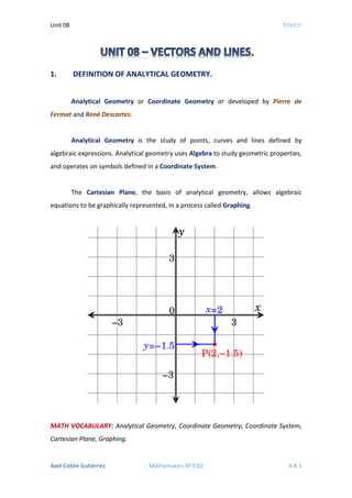
1. Unit 08 March
Axel Cotón Gutiérrez Mathematics 4º ESO 4.8.1
1. DEFINITION OF ANALYTICAL GEOMETRY.
Analytical Geometry or Coordinate Geometry or developed by Pierre de
Fermat and René Descartes.
Analytical Geometry is the study of points, curves and lines defined by
algebraic expressions. Analytical geometry uses Algebra to study geometric properties,
and operates on symbols defined in a Coordinate System.
The Cartesian Plane, the basis of analytical geometry, allows algebraic
equations to be graphically represented, in a process called Graphing.
MATH VOCABULARY: Analytical Geometry, Coordinate Geometry, Coordinate System,
Cartesian Plane, Graphing.

2. Unit 08 March
Axel Cotón Gutiérrez Mathematics 4º ESO 4.8.2
2. VECTORS.
In mathematics, physics, and engineering, a Euclidean Vector is a geometric
object that has Magnitude (or Length) and Direction. A Euclidean Vector is frequently
represented by a line segment with a definite direction, or graphically as an arrow,
connecting an initial point 𝑨 with a terminal point 𝑩, and denoted by 𝑨𝑩⃗⃗⃗⃗⃗⃗ .
2.1. MAGNITUDE AND DIRECTION.
The Magnitude of the vector is the distance between the two points and the
Direction refers to the direction of displacement from 𝑨 to 𝑩.
NOTE: In Spain there are differences between the line that contain the vector called
“dirección” and the side of the arrow, called “sentido”.

3. Unit 08 March
Axel Cotón Gutiérrez Mathematics 4º ESO 4.8.3
2.2. COORDINATES OF A VECTOR.
To find the coordinates of the vector 𝑨𝑩⃗⃗⃗⃗⃗⃗ , that connect point 𝑨(𝒂 𝟏, 𝒂 𝟐) and the
point 𝑩(𝒃 𝟏, 𝒃 𝟐) we have to use this formula:
𝑨𝑩⃗⃗⃗⃗⃗⃗ = (𝒃 𝟏 − 𝒂 𝟏, 𝒃 𝟐 − 𝒂 𝟐)
Find the coordinates of the following vector:
𝐴𝐵⃗⃗⃗⃗⃗ = (𝑥2 − 𝑥1, 𝑦2 − 𝑦1)
𝐴𝐵⃗⃗⃗⃗⃗ = (6 − 2,5 − 2) = (4,3)
2.3. CALCULATING THE MAGNITUDE OF A VECTOR.
If the coordinates of a vector 𝒗⃗⃗ are (𝒗 𝟏, 𝒗 𝟐), its magnitude is:
|𝒗⃗⃗ | = √( 𝒗 𝟏) 𝟐 + (𝒗 𝟐) 𝟐
Find the magnitude of the vector 𝐴𝐵⃗⃗⃗⃗⃗ = (4,3)
|𝐴𝐵⃗⃗⃗⃗⃗ | = √(4)2 + (3)2 = √16 + 9 = √25 = 5

4. Unit 08 March
Axel Cotón Gutiérrez Mathematics 4º ESO 4.8.4
2.4. PARALLEL AND PERPENDICULAR VECTORS.
Two vectors are Parallel when they have the same direction. If 𝒖⃗⃗ = (𝒖 𝟏, 𝒖 𝟐)
and 𝒗⃗⃗ = (𝒗 𝟏, 𝒗 𝟐), 𝒖⃗⃗ and 𝒗⃗⃗ are parallel when their coordinates are proportional:
𝒖 𝟐
𝒖 𝟏
=
𝒗 𝟐
𝒗 𝟏
Two vectors are Perpendicular when their directions cut themselves in a right
angle. If 𝒖⃗⃗ = (𝒖 𝟏, 𝒖 𝟐) and 𝒗⃗⃗ = (𝒗 𝟏, 𝒗 𝟐), 𝒖⃗⃗ and 𝒗⃗⃗ are perpendicular:
𝒖 𝟏 ∙ 𝒗 𝟏 + 𝒖 𝟐 ∙ 𝒗 𝟐 = 𝟎
If we have a vector 𝒖⃗⃗ = (𝒖 𝟏, 𝒖 𝟐), we can find another vector:
 Parallel to 𝒖⃗⃗ by multiplying by a number 𝝀 different to 0: 𝒗⃗⃗ = (𝝀𝒖 𝟏, 𝝀𝒖 𝟐).
 Perpendicular to 𝒖⃗⃗ by reversing their coordinates and changing the sign of one
of them: 𝒗⃗⃗ = (−𝒖 𝟐, 𝒖 𝟏)
MATH VOCABULARY: Vector, Magnitude, Parallel, Perpendicular.
3. OPERATIONS WITH VECTORS.
3.1. ADDING AND SUBTRACTING VECTORS.
To add or subtract two vectors, add or subtract the corresponding
Components. Let 𝒖⃗⃗ = (𝒖 𝟏, 𝒖 𝟐) and 𝒗⃗⃗ = (𝒗 𝟏, 𝒗 𝟐) be two vectors.
Then, the sum of 𝒖⃗⃗ and 𝒗⃗⃗ is the vector:
𝒖⃗⃗ + 𝒗⃗⃗ = (𝒖 𝟏 + 𝒗 𝟏, 𝒖 𝟐 + 𝒗 𝟐)
The difference of 𝒖⃗⃗ and 𝒗⃗⃗ is the vector:

5. Unit 08 March
Axel Cotón Gutiérrez Mathematics 4º ESO 4.8.5
𝒖⃗⃗ − 𝒗⃗⃗ = (𝒖 𝟏 − 𝒗 𝟏, 𝒖 𝟐 − 𝒗 𝟐)
The sum of two or more vectors is called the Resultant. The resultant of two
vectors can be found using either the Parallelogram Method or the Triangle Method.
PARALLELOGRAM METHOD:
Draw the vectors so that their initial points coincide. Then draw lines to form a
complete parallelogram. The diagonal from the initial point to the opposite vertex of
the parallelogram is the resultant.
Vector Addition:
 Place both vectors 𝒖⃗⃗ and 𝒗⃗⃗ at the same initial point.
 Complete the parallelogram. The resultant vector 𝒖⃗⃗ + 𝒗⃗⃗ is the diagonal of the
parallelogram.

6. Unit 08 March
Axel Cotón Gutiérrez Mathematics 4º ESO 4.8.6
Vector Subtraction:
 Complete the parallelogram.
 Draw the diagonals of the parallelogram from the initial point.
TRIANGLE METHOD:
Draw the vectors one after another, placing the initial point of each successive
vector at the terminal point of the previous vector. Then draw the resultant from the
initial point of the first vector to the terminal point of the last vector. This method is
also called the Head-to-Tail Method.
Vector Addition:
Vector Subtraction:

7. Unit 08 March
Axel Cotón Gutiérrez Mathematics 4º ESO 4.8.7
3.2. MULTIPLYING VECTORS BY SCALARS.
Multiplying a vector by a scalar 𝒌 is called Scalar Multiplication. To perform
scalar multiplication, you need to multiply the scalar by each component of the vector.
𝒌 ∙ 𝒖⃗⃗ = (𝒌 ∙ 𝒖 𝟏, 𝒌 ∙ 𝒖 𝟐)
3.3. POSITION VECTOR.
In geometry, a Position or Position Vector, also known as Location Vector or
Radius Vector, is a Euclidean vector that represents the position of a point 𝑨 in space
in relation to an arbitrary reference origin 𝑶.
The addition of a position vector 𝑶𝑨⃗⃗⃗⃗⃗⃗ = (𝒂, 𝒃) and a vector 𝒗⃗⃗ = (𝒗 𝟏, 𝒗 𝟐), give
us another position vector whose coordinates coincide with those of a point 𝑩 that
results from translate the point 𝑨 through vector 𝒗⃗⃗ .

8. Unit 08 March
Axel Cotón Gutiérrez Mathematics 4º ESO 4.8.8
MATH VOCABULARY: Components, Resultant, Parallelogram Method, Triangle
Method, Head-to-Tail Method, Scalar, Scalar Multiplication, Position Vector, Location
Vector, Radius Vector, To Translate.
4. RELATIONS BETWEEN POINTS IN THE PLANE.
4.1. MIDPOINT OF A LINE SEGMENT.
A Line Segment on the coordinate plane is defined by two endpoints whose
coordinates are known. The Midpoint of this segment is exactly halfway between
these endpoints.

9. Unit 08 March
Axel Cotón Gutiérrez Mathematics 4º ESO 4.8.9
Let’s find the coordinates of the midpoint 𝑴 of the segment 𝑨𝑩. Since the two
right triangles must be equal:
𝒙 𝟐 − 𝒙 𝒎 = 𝒙 𝒎 − 𝒙 𝟏 ⇒ 𝟐𝒙 𝒎 = 𝒙 𝟏 + 𝒙 𝟐
𝒙 𝒎 =
𝒙 𝟏 + 𝒙 𝟐
𝟐
𝒚 𝟐 − 𝒚 𝒎 = 𝒚 𝒎 − 𝒚 𝟏 ⇒ 𝟐𝒚 𝒎 = 𝒚 𝟏 + 𝒚 𝟐
𝒚 𝒎 =
𝒚 𝟏 + 𝒚 𝟐
𝟐
The x-coordinate of the midpoint is the average of the x-coordinates of the two
endpoints. The y-coordinate of the midpoint is the average of the y-coordinates of the
two endpoints.

10. Unit 08 March
Axel Cotón Gutiérrez Mathematics 4º ESO 4.8.10
NOTE: If A’ is the Symmetric of A with respect to M, then M is the midpoint of the line
segment AA’.
4.2. COLLINEAR POINTS.
Collinear Points are points that lie on the same straight line. If three points are
collinear, then the two right triangles shown in the picture will be similar. Therefore,
corresponding sides will be in the same ratio.
𝒚 𝟐 − 𝒚 𝟏
𝒙 𝟐 − 𝒙 𝟏
=
𝒚 𝟑 − 𝒚 𝟐
𝒙 𝟑 − 𝒙 𝟐
4.3. DISTANCE BETWEEN TWO POINTS.
To find the distance between any two points 𝑨 and 𝑩, look at the right triangle
in the following picture.

11. Unit 08 March
Axel Cotón Gutiérrez Mathematics 4º ESO 4.8.11
The distance between 𝑨 and 𝑩, 𝒅(𝑨, 𝑩) , is the hypotenuse of the right triangle:
𝒅(𝑨, 𝑩) = √( 𝒙 𝟐 − 𝒙 𝟏) 𝟐 + (𝒚 𝟐 − 𝒚 𝟏) 𝟐
NOTE: Notice that the distance between the points 𝐴 and 𝐵 is the magnitude of the
vector 𝐴𝐵⃗⃗⃗⃗⃗
MATH VOCABULARY: Midpoint, Symmetric, Collinear Points.
5. LINES.
5.1. THE VECTOR EQUATION OF A LINE.
A Line is defined as the set of collinear points on the plane with a point 𝑷, and a
directional vector 𝒗⃗⃗ .

12. Unit 08 March
Axel Cotón Gutiérrez Mathematics 4º ESO 4.8.12
If 𝑷(𝒙 𝟏, 𝒚 𝟏) is a point on the line and the vector 𝑷𝑿⃗⃗⃗⃗⃗⃗ has the same direction as
𝒗⃗⃗ , then:
𝑷𝑿⃗⃗⃗⃗⃗⃗ = 𝒕 ∙ 𝒗⃗⃗ ; 𝒕 ∈ ℝ
But:
𝑷𝑿⃗⃗⃗⃗⃗⃗ = 𝑶𝑿⃗⃗⃗⃗⃗⃗ − 𝑶𝑷⃗⃗⃗⃗⃗⃗
𝑶𝑿⃗⃗⃗⃗⃗⃗ − 𝑶𝑷⃗⃗⃗⃗⃗⃗ = 𝒕 ∙ 𝒗⃗⃗
𝑶𝑿⃗⃗⃗⃗⃗⃗ = 𝑶𝑷⃗⃗⃗⃗⃗⃗ + 𝒕 ∙ 𝒗⃗⃗
(𝒙, 𝒚) = (𝒙 𝟏, 𝒚 𝟏) + 𝒕 ∙ (𝒗 𝟏, 𝒗 𝟐)
The vector 𝒗⃗⃗ = (𝒗 𝟏, 𝒗 𝟐) is called Direction Vector of the line.
Find the vector equation of the line that have the collinear points 𝐴(−1,2) and 𝐵(0,5)
The direction vector of the line is: 𝐴𝐵⃗⃗⃗⃗⃗ = (0 − (−1), 5 − 2) = (1,3)
We choose any point of the line, for example 𝐴(−1,2)
The vector equation is:
(𝑥, 𝑦) = (−1,2) + 𝑡 ∙ (1,3)
5.2. THE PARAMETRIC EQUATIONS OF A LINE.
In mathematics, Parametric Equations define a group of quantities as functions
of one or more independent variables called Parameters. From the vector equation:
(𝒙, 𝒚) = (𝒙 𝟏, 𝒚 𝟏) + 𝒕 ∙ (𝒗 𝟏, 𝒗 𝟐)
𝒙 = 𝒙 𝟏 + 𝒕 ∙ 𝒗 𝟏
𝒚 = 𝒚 𝟏 + 𝒕 ∙ 𝒗 𝟐
}
These ones are the parametric equations of the line.

13. Unit 08 March
Axel Cotón Gutiérrez Mathematics 4º ESO 4.8.13
From the line (𝑥, 𝑦) = (−1,2) + 𝑡 ∙ (1,3), find the parametric equation:
x = −1 + t
y = 2 + 3t
}
5.3. THE SYMMETRIC EQUATIONS OF A LINE.
If we equalize the value of 𝒕 of the parametric equations we obtain the
Symmetric Equations of the line:
𝒙 = 𝒙 𝟏 + 𝒕 ∙ 𝒗 𝟏
𝒚 = 𝒚 𝟏 + 𝒕 ∙ 𝒗 𝟐
} ⇒
𝒕 =
𝒙 − 𝒙 𝟏
𝒗 𝟏
𝒕 =
𝒚 − 𝒚 𝟏
𝒗 𝟐
}
𝒙 − 𝒙 𝟏
𝒗 𝟏
=
𝒚 − 𝒚 𝟏
𝒗 𝟐
We only can use this equation when (𝒗 𝟏, 𝒗 𝟐) ≠ (𝟎, 𝟎). When 𝒗 𝟏 or 𝒗 𝟐 are
equal to zero, the line is parallel to an axis.
Find the symmetric equation of the line of the example above:
x = −1 + t
y = 2 + 3t
}
𝑥 + 1 =
𝑦 − 2
3
5.4. POINT-SLOPE FORM OF THE EQUATION OF A LINE.
If we try to find the value of 𝒚 − 𝒚 𝟏 from the symmetric equations we obtain:
𝒚 − 𝒚 𝟏 = 𝒗 𝟐 ∙
𝒙 − 𝒙 𝟏
𝒗 𝟏
=
𝒗 𝟐
𝒗 𝟏
∙ (𝒙 − 𝒙 𝟏)

14. Unit 08 March
Axel Cotón Gutiérrez Mathematics 4º ESO 4.8.14
𝒚 − 𝒚 𝟏 = 𝒎 ∙ (𝒙 − 𝒙 𝟏)
The value of 𝒎 is called Slope and 𝑷(𝒙 𝟏, 𝒚 𝟏) is a point of the line.
Find the point-slope equation from the example above:
𝑥 + 1 =
𝑦 − 2
3
𝑦 − 2 = 3 ∙ (𝑥 + 1)
The line has slope 𝑚 = 3 and the point 𝑃(−1, 2) is a point that belongs to the line.

15. Unit 08 March
Axel Cotón Gutiérrez Mathematics 4º ESO 4.8.15
5.5. SLOPE-INTERCEPT FORM OF THE EQUATION OF A LINE.
The "𝒃" value (called the Y-Intercept) is where the line crosses the y-axis.
Suppose a non vertical line has slope 𝒎 and y-intercept 𝒃. This means it
intersects the y-axis at the point (𝟎, 𝒃) , so the point-slope form of the equation of
the line, with 𝑷(𝒙 𝟏, 𝒚 𝟏) = (𝟎, 𝒃):
𝒚 − 𝒚 𝟏 = 𝒎 ∙ (𝒙 − 𝒙 𝟏)
𝒚 − 𝒃 = 𝒎 ∙ (𝒙 − 𝟎)
𝒚 − 𝒃 = 𝒎 ∙ 𝒙
𝒚 = 𝒎 ∙ 𝒙 + 𝒃
Find the slope-intercept equation from the example above:
𝑦 − 2 = 3 ∙ (𝑥 + 1)
𝑦 − 2 = 3𝑥 + 3
𝑦 = 3𝑥 + 3 + 2

16. Unit 08 March
Axel Cotón Gutiérrez Mathematics 4º ESO 4.8.16
𝑦 = 3𝑥 + 5
The line has slope 𝑚 = 3 and 𝑦 − 𝑖𝑛𝑡𝑒𝑟𝑐𝑒𝑝𝑡 = 5, that is the line cut the axis in the
point (0,5).
5.6. GENERAL EQUATION OF A LINE.
The General Equation of a line is:
𝑨𝒙 + 𝑩𝒚 + 𝑪 = 𝟎, 𝑨, 𝑩, 𝑪 ∈ ℝ
Find the general equation from the example above:
𝑦 = 3𝑥 + 5
3𝑥 − 𝑦 − 5 = 0
As we can see, 𝐴 = 3, 𝐵 = −1 and 𝐶 = −5
If we find the value of 𝒚 from the General Equation:
𝒚 =
−𝑨𝒙 − 𝑪
𝑩
= −
𝑨𝒙
𝑩
−
𝑪
𝑩
= 𝒎𝒙 + 𝒃
Therefore:
𝒎 = −
𝑨
𝑩
𝒂𝒏𝒅 𝒃 = −
𝑪
𝑩
And
𝒗⃗⃗ = (𝑩, −𝑨) is a Direction Vector of the line.
MATH VOCABULARY: Direction Vector, Vector Equation, Parametric Equation,
Parameters, Symmetric Equations, Point-Slope Equation, Slope, Slope-Intercept
Equation, Y-Intercept, General Equation.

17. Unit 08 March
Axel Cotón Gutiérrez Mathematics 4º ESO 4.8.17
6. RELATIVE POSITON OF TWO LINES.
Two lines can be:
 Intersecting Lines: if they cross at exactly one point in common.
 Parallel Lines: they never cross.
 Coincident Lines: they lie exactly on top of each other
Intersecting Lines
Parallel Lines

18. Unit 08 March
Axel Cotón Gutiérrez Mathematics 4º ESO 4.8.18
Coincident Lines
If we consider the line 𝒓 with the direction vector 𝒖⃗⃗ = (𝒖 𝟏, 𝒖 𝟐) and slope 𝒎,
and the line 𝒔 with the direction vector𝒗⃗⃗ = (𝒗 𝟏, 𝒗 𝟐) and slope 𝒎′:
POSITION DIRECTION VECTORS SLOPES
GENERAL
EQUATION
Parallel
𝑢2
𝑢1
=
𝑣2
𝑣1
𝑚 = 𝑚′
𝐴
𝐴′
=
𝐵
𝐵′
≠
𝐶
𝐶′
Coincident
𝑢2
𝑢1
=
𝑣2
𝑣1
𝑚 = 𝑚′
𝐴
𝐴′
=
𝐵
𝐵′
=
𝐶
𝐶′
Intersecting
𝑢2
𝑢1
≠
𝑣2
𝑣1
𝑚 ≠ 𝑚′
𝐴
𝐴′
≠
𝐵
𝐵′
Find the relative position of:
𝑟:
𝑥 − 1
2
=
𝑦 + 2
1
𝑠: 𝑦 = −2𝑥 − 1
}
The slope of r is 1/2 and the slope of s is −2
1
2
≠ −2 ⇒ 𝐼𝑛𝑡𝑒𝑟𝑠𝑒𝑐𝑡𝑖𝑛𝑔 𝐿𝑖𝑛𝑒𝑠
MATH VOCABULARY: Intersecting Lines, Parallel Lines, Coincident Lines.