P1 APRary P2 APRary QC APRSeptember 15, 1.docx

P1: APR/ary P2: APR/ary QC: APR
September 15, 1998 11:37 Annual Reviews AR067-08
Annu. Rev. Ecol. Syst. 1998. 29:207–31
Copyright c© 1998 by Annual Reviews. All rights reserved
ROADS AND THEIR MAJOR
ECOLOGICAL EFFECTS
Richard T. T. Forman and Lauren E. Alexander
Harvard University Graduate School of Design, Cambridge,
Massachusetts 02138
KEY WORDS: animal movement, material flows, population
effects, roadside vegetation,
transportation ecology
ABSTRACT
A huge road network with vehicles ramifies across the land,
representing a sur-
prising frontier of ecology. Species-rich roadsides are conduits
for few species.
Roadkills are a premier mortality source, yet except for local
spots, rates rarely
limit population size. Road avoidance, especially due to traffic
noise, has a greater
ecological impact. The still-more-important barrier effect
subdivides populations,
with demographic and probably genetic consequences. Road
networks crossing

landscapes cause local hydrologic and erosion effects, whereas
stream networks
and distant valleys receive major peak-flow and sediment
impacts. Chemical ef-
fects mainly occur near roads. Road networks interrupt
horizontal ecological
flows, alter landscape spatial pattern, and therefore inhibit
important interior
species. Thus, road density and network structure are
informative landscape
ecology assays. Australia has huge road-reserve networks of
native vegetation,
whereas the Dutch have tunnels and overpasses perforating road
barriers to en-
hance ecological flows. Based on road-effect zones, an
estimated 15–20% of the
United States is ecologically impacted by roads.
INTRODUCTION
Roads appear as major conspicuous objects in aerial views and
photographs,
and their ecological effects spread through the landscape. Few
environmental
scientists, from population ecologists to stream or landscape
ecologists, recog-
nize the sleeping giant, road ecology. This major frontier and its
applications to
planning, conservation, management, design, and policy are
great challenges
for science and society.
207
0066-4162/98/1120-0207$08.00
A

nn
u.
R
ev
. E
co
l.
S
ys
t.
1
99
8.
29
:2
07
-2
31
. D
ow
nl
oa
de
d

fr
om
a
rj
ou
rn
al
s.
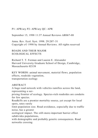
an
nu
al
re
vi
ew
s.
or
g
by
W
ar
sa
w
U
ni

ve
rs
it
y
on
0
3/
24
/0
5.
F
or
p
er
so
na
l
us
e
on
ly
.

208 FORMAN & ALEXANDER
This review often refers to The Netherlands and Australia as
world leaders
with different approaches in road ecology and to the United
States for es-
pecially useful data. In The Netherlands, the density of main
roads alone is
1.5 km/km2, with traffic density of generally between 10,000
and 50,000 ve-
hicles per commuter day (101). Australia has nearly 900,000 km
of roads for
18 million people (66). In the United States, 6.2 million km of
public roads
are used by 200 million vehicles (85). Ten percent of the road
length is in
national forests, and one percent is interstate highways. The
road density is
1.2 km/km2, and Americans drive their cars for about 1 h/day.
Road density is
increasing slowly, while vehicle kilometers (miles) traveled
(VMT) is growing
rapidly.
The term road corridor refers to the road surface plus its
maintained roadsides
and any parallel vegetated strips, such as a median strip
between lanes in a
highway (Figure 1; see color version at end of volume).
“Roadside natural
strips” of mostly native vegetation receiving little maintenance

and located
adjacent to roadsides are common in Australia (where road
corridors are called
road reserves) (12, 39, 111). Road corridors cover
approximately 1% of the
United States, equal to the area of Austria or South Carolina
(85). However,
the area directly affected ecologically is much greater (42, 43).
Theory for road corridors highlights their functional roles as
conduits, bar-
riers (or filters), habitats, sources, and sinks (12, 39). Key
variables affecting
processes are corridor width, connectivity, and usage intensity.
Network theory,
in turn, focuses on connectivity, circuitry, and node functions
(39, 71).
This review largely excludes road-construction-related
activities, as well
as affiliated road features such as rest stops, maintenance
facilities, and en-
trance/exit areas. We also exclude the dispersed ecological
effects of air pollu-
tion emissions, such as greenhouse gases, nitrogen oxides
(NOX), and ozone,
which are reviewed elsewhere (85, 135). Bennett’s article (12)
plus a series of
books (1, 21, 33, 111) provide overviews of parts of road
ecology.
Gaping holes in our knowledge of road ecology represent
research oppor-
tunities with a short lag between theory and application. Current
ecological
knowledge clusters around five major topics: (a) roadsides and

adjacent strips;
(b) road and vehicle effects on populations; (c) water, sediment,
chemicals, and
streams; (d ) the road network; and (e) transportation policy and
planning.
−−−−−−−−−−−−−−−−−−−−−−−−−−−−−−−−−−−−−−−−−−−−−−−
−−−−−−−→
Figure 1 Road corridor showing road surface, maintained open
roadsides, and roadside natural
strips. Strips of relatively natural vegetation are especially
characteristic of road corridors (known
as road reserves) in Australia. Wheatbelt of Western Australia.
Photo courtesy of BMJ Hussey.
See color version at end of volume.
A
nn
u.
R
ev
. E
co
l.
S
ys
t.
1
99
8.

29
:2
07
-2
31
. D
ow
nl
oa
de
d
fr
om
a
rj
ou
rn
al
s.
an
nu
al
re
vi

ew
s.
or
g
by
W
ar
sa
w
U
ni
ve
rs
it
y
on
0
3/
24
/0
5.
F
or
p

er
so
na
l
us
e
on
ly
.
P1: KKK
October 14, 1998 15:2 Annual Reviews AR066-18
ROADS AND ECOLOGICAL EFFECTS 209
A
nn
u.
R
ev
. E
co
l.

S
ys
t.
1
99
8.
29
:2
07
-2
31
. D
ow
nl
oa
de
d
fr
om
a
rj
ou
rn
al

s.
an
nu
al
re
vi
ew
s.
or
g
by
W
ar
sa
w
U
ni
ve
rs
it
y
on
0
3/

24
/0
5.
F
or
p
er
so
na
l
us
e
on
ly
.
ROADSIDE VEGETATION AND ANIMALS
Plants and Vegetation
“Roadside” or “verge” refers to the more-or-less intensively

managed strip,
usually dominated by herbaceous vegetation, adjacent to a road
surface
(Figure 1). Plants on this strip tend to grow rapidly with ample
light and with
moisture from road drainage. Indeed, management often
includes regular mow-
ing, which slows woody-plant invasion (1, 86). Ecological
management may
also maintain roadside native-plant communities in areas of
intensive agricul-
ture, reduce the invasion of exotic (non-native) species, attract
or repel animals,
enhance road drainage, and reduce soil erosion.
Roadsides contain few regionally rare species but have
relatively high plant
species richness (12, 139). Disturbance-tolerant species
predominate, espe-
cially with intensive management, adjacent to highways, and
exotic species
typically are common (19, 121). Roadside mowing tends to both
reduce plant
species richness and favor exotic plants (27, 92, 107).
Furthermore, cutting and
removing hay twice a year may result in higher plant species
richness than does
mowing less frequently (29, 86). Native wildflower species are
increasingly
planted in dispersed locations along highways (1).
Numerous seeds are carried and deposited along roads by
vehicles (70, 112).
Plants may also spread along roads due to vehicle-caused air
turbulence
(107, 133) or favorable roadside conditions (1, 92, 107, 121,

133). For exam-
ple, the short-distance spread of an exotic wetland species,
purple loosestrife
(Lythrum salicaria), along a New York highway was facilitated
by roadside
ditches, as well as culverts connecting opposite sides of the
highway and the
median strip of vegetation (133). Yet few documented cases are
known of
species that have successfully spread more than 1 km because of
roads.
Mineral nutrient fertilization from roadside management, nearby
agriculture,
and atmospheric NOX also alter roadside vegetation. In Britain,
for example,
vegetation was changed for 100–200 m from a highway by
nitrogen from traffic
exhaust (7). Nutrient enrichment from nearby agriculture
enhances the growth
of aggressive weeds and can be a major stress on a roadside
native-plant commu-
nity (19, 92). Indeed, to conserve roadside native-plant
communities in Dutch
farmland, fertilization and importing topsoil are ending, and in
some places
nutrient accumulations and weed seed banks are reduced by soil
removal (86;
H van Bohemen, personal communication).
Woody species are planted in some roadsides to reduce erosion,
control
snow accumulation, support wildlife, reduce headlight glare, or
enhance aes-
thetics (1, 105). Planted exotic species, however, may spread
into nearby natural

ecosystems (3, 12). For example, in half the places where non-
native woody
species were planted in roadsides adjacent to woods in
Massachusetts (USA),
a species had spread into the woods (42).
A
nn
u.
R
ev
. E
co
l.
S
ys
t.
1
99
8.
29
:2
07
-2
31
. D

ow
nl
oa
de
d
fr
om
a
rj
ou
rn
al
s.
an
nu
al
re
vi
ew
s.
or
g
by
W

ar
sa
w
U
ni
ve
rs
it
y
on
0
3/
24
/0
5.
F
or
p
er
so
na
l
us
e

on
ly
.
Roadside management sometimes creates habitat diversity to
maintain native
ecosystems or species (1, 86, 131). Mowing different sections
along a road, or
parallel strips in wide roadsides, at different times or intervals
may be quite ef-
fective (87). Ponds, wetlands, ditches, berms, varied roadside
widths, different
sun and shade combinations, different slope angles and
exposures, and shrub
patches rather than rows offer variety for roadside species
richness.
In landscapes where almost all native vegetation has been
removed for cul-
tivation or pasture, roadside natural strips (Figure 1) are
especially valuable as
reservoirs of biological diversity (19, 66). Strips of native
prairie along roads
and railroads, plus so-called beauty strips of woodland that
block views near
intensive logging, may function similarly as examples.

However, roadside nat-
ural strips of woody vegetation are widespread in many
Australian agricultural
landscapes and are present in South Africa (11, 12, 27, 39, 66,
111). Overall,
these giant green networks provide impressive habitat
connectivity and disperse
“bits of nature” widely across a landscape. Yet they miss the
greater ecological
benefits typically provided by large patches of natural
vegetation (39, 41).
In conclusion, roadside vegetation is rich in plant species,
although appar-
ently not an important conduit for plants. The scattered
literature suggests a
promising research frontier.
Animals and Movement Patterns
Mowing, burning, livestock grazing, fertilizing, and planting
woody plants
greatly impact native animals in roadsides. Cutting and
removing roadside veg-
etation twice a year in The Netherlands, compared with less
frequent mowing,
results in more species of small mammals, reptiles, amphibians,
and insects
(29, 86). However, mowing once every 3–5 y rather than
annually results
in more bird nests. Many vertebrate species persist better with
mowing af-
ter, rather than before or during, the breeding period (86, 87).
The mowing
regime is especially important for insects such as meadow
butterflies and moths,
where different species go through stages of their annual cycle

at different times
(83). Roadsides, especially where mowed cuttings are removed,
are suitable
for ∼80% of the Dutch butterfly fauna (86).
Planting several native and exotic shrub species along Indiana
(USA)
highways resulted in higher species richness, population
density, and nest den-
sity for birds, compared with nearby grassy roadsides (105).
Rabbit (Sylvilagus)
density increased slightly. However, roadkill rates did not differ
next to shrubby
versus grassy roadsides.
In general, road surfaces, roadsides, and adjacent areas are little
used as
conduits for animal movement along a road (39), although
comparisons with
null models are rare. For example, radiotracking studies of
wildlife across the
landscape detect few movements along or parallel to roads (35,
39, 93). Some
exceptions are noteworthy. Foraging animals encountering a
road sometimes
A
nn
u.
R
ev
. E
co

l.
S
ys
t.
1
99
8.
29
:2
07
-2
31
. D
ow
nl
oa
de
d
fr
om
a
rj
ou
rn

al
s.
an
nu
al
re
vi
ew
s.
or
g
by
W
ar
sa
w
U
ni
ve
rs
it
y
on
0

3/
24
/0
5.
F
or
p
er
so
na
l
us
e
on
ly
.
move short distances parallel to it (10, 106). At night, many
large predator

species move along roads that have little vehicular or people
traffic (12, 39).
Carrion feeders move along roads in search of roadkills, and
vehicles some-
times transport amphibians and other animals (11, 12, 32).
Small mammals
have spread tens of kilometers along highway roadsides (47,
60). In addition,
migrating birds might use roads as navigational cues.
Experimental, observational, and modeling approaches have
been used to
study beetle movement along roadsides in The Netherlands
(125–127). On wide
roadsides, fewer animals disappeared into adjacent habitats.
Also, a dense grass
strip by the road surface minimized beetle susceptibility to
roadkill mortality
(126, 127). Long dispersals of beetles were more frequent in
wide (15–25 m)
than in narrow (<12 m) roadsides. Nodes of open vegetation
increased, and
narrow bottlenecks decreased, the probability of long dispersals.
The results
suggest that with 20–30-m-wide roadsides containing a central
suitable habitat,
beetle species with poor dispersal ability and a good
reproductive rate may
move 1–2 km along roadsides in a decade (127).
Adjacent ecosystems also exert significant influences on
animals in corridors
(39). For example, roadside beetle diversity was higher near a
similar patch
of sandy habitat, and roadsides next to forest had the greatest
number of forest

beetle species (127). In an intensive-agriculture landscape
(Iowa, USA), bird-
nest predation in roadsides was highest opposite woods and
lowest opposite
pastures (K Freemark, unpublished data). Finally, some roadside
animals also
invade nearby natural vegetation (37, 47, 54, 60, 63, 127).
The median strip between lanes of a highway is little studied. A
North
Carolina (USA) study found no difference in small-mammal
density between
roadsides on the median and on the outer side of the highway
(2). This result was
the same whether comparing mowed roadside areas or unmowed
roadside areas.
Also, roadkill rates may be affected by the pattern of wooded
and grassy areas
along median strips (10).
In conclusion, some species move significant distances along
roadsides and
have major local impacts. Nevertheless, road corridors appear to
be relatively
unimportant as conduits for species movement, although
movement rates should
be better compared with those at a distance and in natural-
vegetation corridors.
ROAD AND VEHICLE EFFECTS ON POPULATIONS
Roadkilled Animals
Sometime during the last three decades, roads with vehicles
probably overtook
hunting as the leading direct human cause of vertebrate
mortality on land. In

addition to the large numbers of vertebrates killed, insects are
roadkilled in
prodigious numbers, as windshield counts will attest.
A
nn
u.
R
ev
. E
co
l.
S
ys
t.
1
99
8.
29
:2
07
-2
31
. D
ow
nl

oa
de
d
fr
om
a
rj
ou
rn
al
s.
an
nu
al
re
vi
ew
s.
or
g
by
W
ar
sa

w
U
ni
ve
rs
it
y
on
0
3/
24
/0
5.
F
or
p
er
so
na
l
us
e
on
ly

.
Estimates of roadkills (faunal casualties) based on
measurements in short
sections of roads tell the annual story (12, 39, 123): 159,000
mammals and
653,000 birds in The Netherlands; seven million birds in
Bulgaria; five million
frogs and reptiles in Australia. An estimated one million
vertebrates per day
are killed on roads in the United States.
Long-term studies of roadkills near wetlands illustrate two
important pat-
terns. One study recorded>625 snakes and another>1700 frogs
annually
roadkilled per kilometer (8, 54). A growing literature suggests
that roads by
wetlands and ponds commonly have the highest roadkill rates,
and that, even
though amphibians may tend to avoid roads (34), the greatest
transportation
impact on amphibians is probably roadkills (8, 28, 34, 128).
Road width and vehicle traffic levels and speeds affect roadkill
rates. Am-

phibians and reptiles tend to be particularly susceptible on two-
lane roads with
low to moderate traffic (28, 34, 57, 67). Large and mid-sized
mammals are espe-
cially susceptible on two-lane, high-speed roads, and birds and
small mammals
on wider, high-speed highways (33, 90, 106).
Do roadkills significantly impact populations? Measurements of
bird and
mammal roadkills in England illustrate the main pattern (56,
57). The house
sparrow (Passer domesticus) had by far the highest roadkill rate.
Yet this species
has a huge population, reproduces much faster than the roadkill
rate, and can
rapidly recolonize locations where a local population drops. The
study con-
cluded, based on the limited data sets available, that none of
the>100 bird and
mammal species recorded had a roadkill rate sufficient to affect
population size
at the national level.
Despite this overall pattern, roadkill rates are apparently
significant for a few
species listed as nationally endangered or threatened in various
nations (∼9–
12 cases) (9, 39, 43; C Vos, personal communication). Two
examples from
southern Florida (USA) are illustrative. The Florida panther
(Felis concolor
coryi) had an annual roadkill mortality of approximately 10% of
its population
before 1991 (33, 54). Mitigation efforts reduced roadkill loss to
2%. The key

deer (Odocoileus virginianus clavium) has an annual roadkill
mortality of∼16%
of its population. Local populations, of course, may suffer
declines where the
roadkill rate exceeds the rates of reproduction and immigration.
At least a dozen
local-population examples are known for vertebrates whose
total populations
are not endangered (33, 39, 43).
Vehicles often hit vertebrates attracted to spilled grain, roadside
plants, in-
sects, basking animals, small mammals, road salt, or dead
animals (12, 32, 56,
87). Roadkills may be frequent where traffic lanes are separated
by imperme-
able barriers or are between higher roadside banks (10, 106).
Landscape spatial patterns also help determine roadkill
locations and rates.
Animals linked to specific adjacent land uses include
amphibians roadkilled
A
nn
u.
R
ev
. E
co
l.
S

ys
t.
1
99
8.
29
:2
07
-2
31
. D
ow
nl
oa
de
d
fr
om
a
rj
ou
rn
al
s.

an
nu
al
re
vi
ew
s.
or
g
by
W
ar
sa
w
U
ni
ve
rs
it
y
on
0
3/
24

/0
5.
F
or
p
er
so
na
l
us
e
on
ly
.
near wetlands and turtles near open-water areas (8). Foraging
deer are often
roadkilled between fields in forested landscapes, between
wooded areas in
open landscapes, or by conservation areas in suburbs (10, 42,

106). The vicinity
of a large natural-vegetation patch and the area between two
such patches are
likely roadkill locations for foraging or dispersing animals.
Even more likely
locations are where major wildlife-movement routes are
interrupted, such as
roads crossing drainage valleys in open landscapes or crossing
railway routes
in suburbs (42, 106).
In short, road vehicles are prolific killers of terrestrial
vertebrates. Neverthe-
less, except for a small number of rare species, roadkills have
minimal effect
on population size.
Vehicle Disturbance and Road Avoidance
The ecological effect of road avoidance caused by traffic
disturbance is probably
much greater than that of roadkills seen splattered along the
road. Traffic noise
seems most important, although visual disturbance, pollutants,
and predators
moving along a road are alternative hypotheses as the cause of
avoidance.
Studies of the ecological effects of highways on avian
communities in The
Netherlands point to an important pattern. In both woodlands
and grasslands
adjacent to roads, 60% of the bird species present had a lower
density near a
highway (102, 103). In the affected zone, the total bird density
was approxi-
mately one third lower, and species richness was reduced as

species progres-
sively disappeared with proximity to the road. Effect-distances
(the distance
from a road at which a population density decrease was
detected) were greatest
for birds in grasslands, intermediate for birds in deciduous
woods, and least for
birds in coniferous woods.
Effect-distances were also sensitive to traffic density. Thus,
with an average
traffic speed of 120 km/h, the effect-distances for the most
sensitive species
(rather than for all species combined) were 305 m in woodland
by roads with
a traffic density of 10,000 vehicles per day (veh/day) and 810 m
in woodland by
50,000 veh/day; 365 m in grassland by 10,000 veh/day and 930
m in grassland
by 50,000 veh/day (101–103). Most grassland species showed
population de-
creases by roads with 5000 veh/day or less (102). The effect-
distances for both
woodland and grassland birds increased steadily with average
vehicle speed
up to 120 km/h and also with traffic density from 3000 to
140,000 veh/day
(100, 102, 103). These road effects were more severe in years
when overall bird
population sizes were low (101).
Songbirds appear to be sensitive to remarkably low noise levels,
similar to
those in a library reading room (100, 102, 103). The noise level
at which popula-
tion densities of all woodland birds began to decline averaged

42 decibels (dB),
compared with an average of 48 dB for grassland species. The
most sensitive
A
nn
u.
R
ev
. E
co
l.
S
ys
t.
1
99
8.
29
:2
07
-2
31
. D
ow
nl

.
woodland species (cuckoo) showed a decline in density at 35
dB, and the
most sensitive grassland bird (black-tailed godwit,Limosa
limosa) responded
at 43 dB. Field studies and experiments will help clarify the
significance of
these important results for traffic noise and birds.
Many possible reasons exist for the effects of traffic noise.
Likely hypotheses
include hearing loss, increase in stress hormones, altered
behaviors, interfer-
ence with communication during breeding activities, differential
sensitivity to
different frequencies, and deleterious effects on food supply or
other habitat at-
tributes (6, 101, 103, 130). Indeed, vibrations associated with
traffic may affect
the emergence of earthworms from soil and the abundance of
crows (Corvus)
feeding on them (120). A different stress, roadside lighting,
altered nocturnal
frog behavior (18). Responses to roads with little traffic may
resemble behav-

ioral responses to acute disturbances (individual vehicles
periodically passing),
rather than the effects of chronic disturbance along busy roads.
Response to traffic noise is part of a broader pattern of road
avoidance by
animals. In the Dutch studies, visual disturbance and pollutants
extended out-
ward only a short distance compared with traffic noise (100,
103). However,
visual disturbance and predators moving along roads may be
more significant
by low-traffic roads.
Various large mammals tend to have lower population densities
within
100–200 m of roads (72, 93, 108). Other animals that seem to
avoid roads in-
clude arthropods, small mammals, forest birds, and grassland
birds (37, 47, 73,
123). Such road-effect zones, extending outward tens or
hundreds of meters
from a road, generally exhibit lower breeding densities and
reduced species rich-
ness compared with control sites (32, 101). Considering the
density of roads
plus the total area of avoidance zones, the ecological impact of
road avoidance
must well exceed the impact of either roadkills or habitat loss in
road corridors.
Barrier Effects and Habitat Fragmentation
All roads serve as barriers or filters to some animal movement.
Experiments
show that carabid beetles and wolf spiders (Lycosa) are blocked
by roads as

narrow as 2.5 m wide (73), and wider roads are significant
barriers to crossing for
many mammals (11, 54, 90, 113). The probability of small
mammals crossing
lightly traveled roads 6–15 m wide may be<10% of that for
movements within
adjacent habitats (78, 119). Similarly, wetland species,
including amphibians
and turtles, commonly show a reduced tendency to cross roads
(34, 67).
Road width and traffic density are major determinants of the
barrier effect,
whereas road surface (asphalt or concrete versus gravel or soil)
is generally
a minor factor (34, 39, 73, 90). Road salt appears to be a
significant deterrent
to amphibian crossing (28, 42). Also, lobes and coves in
convoluted outer-
roadside boundaries probably affect crossing locations and rates
(39).
A
nn
u.
R
ev
. E
co
l.
S
ys

t.
1
99
8.
29
:2
07
-2
31
. D
ow
nl
oa
de
d
fr
om
a
rj
ou
rn
al
s.
an

nu
al
re
vi
ew
s.
or
g
by
W
ar
sa
w
U
ni
ve
rs
it
y
on
0
3/
24
/0

5.
F
or
p
er
so
na
l
us
e
on
ly
.
The barrier effect tends to create metapopulations, e.g. where
roads divide
a large continuous population into smaller, partially isolated
local populations
(subpopulations) (6, 54, 128). Small populations fluctuate more
widely over

time and have a higher probability of extinction than do large
populations
(1, 88, 115, 122, 123). Furthermore, the recolonization process
is also blocked
by road barriers, often accentuated by road widening or
increases in traffic. This
well-known demographic threat must affect numerous species
near an extensive
road network, yet is little studied relative to roads (6, 73, 98).
The genetics of a population is also altered by a barrier that
persists over many
generations (73, 115). For instance, road barriers altered the
genetic structure
of small local populations of the common frog (Rana
temporaria) in Germany
by lowering genetic heterozygosity and polymorphism (97, 98).
Other than the
barrier effect on this amphibian and roadkill effects on two
southern Florida
mammals (20, 54), little is known of the genetic effects of
roads.
Making roads more permeable reduces the demographic threat
but at the
cost of more roadkills. In contrast, increasing the barrier effect
of roads re-
duces roadkills but accentuates the problems of small
populations. What is the
solution to this quandary (122, 128)? The barrier effect on
populations proba-
bly affects more species, and extends over a wider land area,
than the effects
of either roadkills or road avoidance. This barrier effect may
emerge as the
greatest ecological impact of roads with vehicles. Therefore,

perforating roads
to diminish barriers makes good ecological sense.
WATER, SEDIMENT, CHEMICALS, STREAMS,
AND ROADS
Water Runoff
Altering flows can have major physical or chemical effects on
aquatic ecosys-
tems. The external forces of gravity and resistance cause
streams to carve chan-
nels, transport materials and chemicals, and change the
landscape (68). Thus,
water runoff and sediment yield are the key physical processes
whereby roads
have an impact on streams and other aquatic systems, and the
resulting effect-
distances vary widely (Figure 2).
Roads on upper hillslopes concentrate water flows, which in
turn form chan-
nels higher on slopes than in the absence of roads (80). This
process leads to
smaller, more elongated first-order drainage basins and a longer
total length
of the channel network. The effects of stream network length on
erosion and
sedimentation vary with both scale and drainage basin area (80).
Water rapidly runs off relatively impervious road surfaces,
especially in storm
and snowmelt events. However, in moist, hilly, and
mountainous terrain, such
A
nn

u.
R
ev
. E
co
l.
S
ys
t.
1
99
8.
29
:2
07
-2
31
. D
ow
nl
oa
de
d
fr

om
a
rj
ou
rn
al
s.
an
nu
al
re
vi
ew
s.
or
g
by
W
ar
sa
w
U
ni
ve

rs
it
y
on
0
3/
24
/0
5.
F
or
p
er
so
na
l
us
e
on
ly
.

Figure 2 Road-effect zone defined by ecological effects
extending different distances from a road.
Most distances are based on specific illustrative studies (39);
distance to left is arbitrarily half of
that to right. (P) indicates an effect primarily at specific points.
From Forman et al (43).
runoff is often insignificant compared with the conversion of
slow-moving
groundwater to fast-moving surface water at cutbanks by roads
(52, 62, 132).
Surface …
FEASIBILITY REPORT 1
FEASIBILITY REPORT 6
Feasibility Report

MEMO
TO: Manager
FROM:
DATE:
SUBJECT:
This memo is meant for introducing the feasibility report that
aims at providing a solution to the cases and nation problems
about the cybercrime and the potential proposed solution to curb
up the challenge. These feasibilities we are identified by
studying various critical factors such as the social effects, legal
issues, technical problems, and the economic impact. Therefore,
this memo is very vital for an individual to read and understand
various aspects.
Feasibility Report
It takes much time in planning and preparing to implement a
solution to the major problem in society. During the planning
and preparation process, the proposed solution should be tested
and determined if it is feasible to provide the solution or not.
Cybercrime in united states has been a significant problem and
need to be addressed and solution provided to reduce the
cybercrime.
One of the proposed solutions to this major problem is
providing cybersecurity among very individual. This will enable
most of the people to understand and know the importance of

cybersecurity and thus leading to the reduction of the negative
loses that is caused by the cybercrime in society every year.
Another thing that will ensure that the individuals in the nation
are protected from the impact of the cybercrime is educating
them on ways they can protect themselves over the cybercrime
attempts.
This report will majorly focus on looking at the proposed
solution provided and determine if the answers are feasible or
need some changes. The essential aspects that the story will
focus on include the social impact, the economic effect, and
other elements which will be determined if it can provide a
solution to the problem.
The Social Impact
When looking for a potential solution to be implemented to
solve a specific major problem in society, a positive impact is
always the main objective. When the proposed solution is
applied, such as implementing cybersecurity in the daily lives
of the individuals in the society it will bring a lot of positive
impacts on them. For instance, when the cybersecurity is made
the main focus in the in every place, i.e. schools and workplace,
majority of the individuals will be aware of these threats and
ways of preventing them from affecting their daily lives. This
will also reduce the loss that most of the individuals incur due
to the cybercrime and lack of security in their day-to-day
business operations (Help Net Security, 2015).
When the cybersecurity is introduced in society It will bring
much social impact to the life of the individuals since it will
educate people about the dynamic changes that occur in uses of
the technology. When this provides a solution to the cybercrime
problem in the society, it will be adopted by every nation, and
thus the cybercrime problem is reduced and making every
country secure and safe from the cybercrime problems.
Economic Effect.
One of the most critical aspects of coming up with the proposed
solution is the economic feasibility impact. The projected
resolution calls for basically a change in lifestyle in the United

States. The cybersecurity needs to be the main part of the
individuals that will make them safe and preventing the
occurrence of cybercrime. The cybersecurity has to be
implemented in the workplace and various institutions to
achieve the required objectives of solving the issue of
cybercrime in society.
The process of implementation has a great financial cost, but
the results brought by the proposed solution will bring much
economical cost since it will reduce the amount that could have
been used to solve the loss and cases caused by the cybercrime
in the society. When the financial loss incurred due to the
cybercrime is compared to the cost of implementing the
solution, there is a significant difference since the proposed
solution implementation saves much money.
Technical and Legal Issues
For every proposed solution, becoming successful in solving the
intended problem, there are several legal and professional issues
to be followed during the process of implementation. To
implement cybersecurity in the workplaces and the institutions,
some legal issues have to be developed for it to be successful.
Also, during the process of implementation of the
cybersecurity, the technical aspects have to be looked at. The
technical issues involve various aspects such as unforeseen
failure of the system in providing the solution for the problem.
The technical issues will also identify the bugs that will prevent
the proposed solution from providing the solution to the major
problem. The proposed solutions seem to be free from the
technical and legal issues, and thus it may provide the required
solution to the major problem of cybercrime in the United
States.
Conclusion
Generally, the proposed solution to the major problem of
Cybercrime in the United States is more feasible. The problem
in achieving the solution is the lack of financial support during

the process of implementation of the proposed solution. If the
proposed solution gets financial support, it requires, and it will
be easy to implement it and bring the required resolution.
However, considering all other criteria measured to determine
the feasibility of the proposed solution, I found that
implementing the solution either caused little to no impact or
had a positive effect, such as the case with Social implications.
From the above observation, if there will be no financial
distress during the implementation process, the proposed
solution will be successful in solving the major problem of
cybersecurity.
References
Statistica Research Department. (Published August 9, 2019).
Spending on Cybersecurity in the United States from 2010 to
2018. Statistica.
Retrieved from
https://www.statista.com/statistics/615450/cybersecurity-
spending-in-the-us/
Clement, J. (Published July 9, 2019). Amount of monetary
damage caused by reported cybercrime to the IC3 from 2001 to
2018. Statistica.
Retrieved from https://www.statista.com/statistics/267132/total-
damage-caused-by-by-cyber-crime-in-the-us/
Bada, M. & Nurse, J. (Accessed February 2020). The Social and
Psychological Impact of
Cyber-Attacks. Emerging Cyber Threats and Cognitive
Vulnerabilities.
Retrieved from
https://arxiv.org/ftp/arxiv/papers/1909/1909.13256.pdf
Help Net Security. (Published February 26, 2015). The business
and social impacts of cybersecurity issues.
Retrieved from
https://www.helpnetsecurity.com/2015/02/26/the-business-and-
social-impacts-of-cyber-security-issues/

Chapter 16: Technical Reading Chapter Introduction
Book Title: Technical Writing for Success
Learning, Cengage LearningChapter Introduction
Goals
Explain the difference between technical reading and literary
reading
Preview and anticipate material before you read
Use strategies for reading technical passages
Terms
acronyms (letters that stand for a long or complicated term or
series of terms) annotating (handwritten notes, often placed in
the margins of a document being read) anticipate (to guess or
predict before actually reading a passage what kind of reasoning
it might present)
background knowledge (knowledge and vocabulary that a reader
has already learned and then calls upon to better understand
new information)
formal outline (a listing of main ideas and subtopics arranged in
a traditional format of Roman numerals, capital letters,
numbers, and lowercase letters)
graphic organizers (the use of circles, rectangles, and
connecting lines in notes to show the relative importance of one
piece of information to another)
informal outline (a listing of main ideas and subtopics arranged
in a less traditional format of single headings and indented
notes)
literary reading (reading literature such as short stories, essays,
poetry, and novels) pace (to read efficiently; to read at a rate
that is slow enough to allow the mind to absorb information but
fast enough to complete the reading assignment)
previewing (looking over a reading assignment before reading
it; determining the subject matter and any questions about the
material before reading it) technical reading (reading science,
business, or technology publications)

technical vocabulary (specialized words used in specific ways
unique to a particular discipline)
Write to Learn
How does a science or computer textbook differ from a work of
literature? Do you read scientific or technical material
differently from the way you read literature? If so, how? Do you
like to read? Why or why not? How often do you read scientific
or technical information? How do you remember what you read?
Write a journal entry addressing these questions.
Focus on Technical Reading
Read Figure 16.1 and answer these questions:
What features of technical writing do you recognize in the
passage?
What has the reader done to interact with and understand this
passage?
What kind of information has the reader noted?
What If?
How might the model change if …
The passage included more technical vocabulary?
The information in the passage was part of a presentation on
satellites?
The passage included a couple of graphics?
Figure 16.1
Sample of Technical Reading
Source: From Essentials of Oceanography by Garrison, 2009.
Reprinted with permission of Brooks/Cole, Cengage Learning.
Writing @Work
Courtesy of Stephen Freas
Source: The Center to Advance CTE
Stephen Freas is a construction subcontractor in Winston Salem,
North Carolina. He is a supervisor on job sites and manages
small crews to build projects based on drawings provided by the

general contractor. He writes contracts, e-mails with clients,
and often consults manuals and building codes.
The contracts Stephen writes are more than just fine print to be
skimmed and signed. “A contract lets the client know exactly
what we’re going to do—what materials and processes will be
necessary, what those will cost, and what the potential risks
are,” says Stephen. “A detailed contract also prevents us from
doing costly work for free.”
Stephen’s job requires him to do a great deal of technical
reading. “Reading construction plans and technical manuals
requires a physical engagement with the writing,” he says. “In
these texts, an action usually follows each sentence or image.
This makes for slow but ‘action-packed’ reading that helps you
accomplish something you had no idea how to do previously.”
Stephen often combines information gleaned from several
different pieces of technical writing in order to make proper
decisions. For example, “Once, we built a handicap ramp to the
specifications written by the contractor. Upon inspection, the
city told us that the ramp did not meet its building code
standards. I refused to rebuild the ramp until I read the city
code myself. The code listed specifics such as ramp thickness;
railing height; and, most important, ramp slope. I calculated
that in order to meet city code specifications, the ramp needed
to be three times longer than the contractor’s original plan and,
coincidentally, the same slope as the existing sidewalk.”
Stephen credits his technical reading dexterity to countless
hours of following instruction manuals for his car, photography,
climbing, and other hobbies.
Think Critically
1. Why does Stephen consider construction plans and technical
manuals to be “action-packed”?
2. Think about the completed handicap ramp from the point of
view of Stephen, the general contractor, and the building
inspector. What solution would work for everyone?
Printed with permission of Stephen Freas
Writing in Architecture and Construction Building contractors

plan, coordinate, and supervise construction projects. Writing
consists of evaluating the job site and scope of work; designing
specifications with accompanying photos; and creating bid
documents, change orders, and general correspondence.
Evaluations assess the feasibility of the project considering
such things as removal of asbestos for renovations or placement
of sewer lines for new construction. The scope of work
pinpoints the responsibilities of the contractor. For example, the
contractor may or may not be responsible for landscaping,
depending on the agreement reached.
Putting in writing the exact building specifications and
accompanying costs is an essential task for a contractor. For
example, the description of the wooden steps should be precise
and clear to prevent misunderstandings later: “A new set of
timber-framed steps with hand rails (meeting the SC Residential
Building Code) will be added within the porch to access the
porch from the front door (to replace existing concrete steps.”
Change orders revise the initial plan when a homeowner wants
to add something, such as a half bath, or when a problem arises
that neither the contractor nor homeowner foresaw. Once the
project is underway, the contractor’s ability to convey clear
instructions to workers is critical.
Estimating costs may be the most difficult part of the
contractor’s job. Contractors research all current material costs
and subcontractors’ estimates. They need a realistic
understanding of the time to complete the project. Whether
calculating time and materials or a turn-key contract price,
builders estimate costs carefully and include a sufficient profit
margin—or risk losing money.
Chapter 16: Technical Reading Chapter Introduction
Book Title: Technical Writing for Success
Printed By: Henry Mack ([email protected]) © 2019 Cengage
Learning, Cengage Learning
© 2020 Cengage Learning Inc. All rights reserved. No part of
this work may by reproduced or used in any form or by any
means graphic, electronic, or mechanical, or in any other

manner - without the written permission of the copyright holder.
Fire as a global ‘herbivore’: the ecology
and evolution of flammable
ecosystems
William J. Bond
1
and Jon E. Keeley
2,3
1
Department of Botany, University of Cape Town, Rondebosch,
South Africa
2
U.S.GeologicalSurvey, Western Ecological ResearchCenter,
Sequoia-Kings Canyon National Parks,Three Rivers, CA93271-
9651, USA
3
Department of Ecology and Evolutionary Biology, University of
California, Los Angeles, CA 90095, USA
It is difficult to find references to fire in general
textbooks on ecology, conservation biology or biogeo-
graphy, in spite of the fact that large parts of the world
burn on a regular basis, and that there is a considerable
literature on the ecology of fire and its use for managing

ecosystems. Fire has been burning ecosystems for
hundreds of millions of years, helping to shape global
biome distribution and to maintain the structure and
function of fire-prone communities. Fire is also a
significant evolutionary force, and is one of the first
tools that humans used to re-shape their world. Here,
we review the recent literature, drawing parallels
between fire and herbivores as alternative consumers
of vegetation. We point to the common questions, and
some surprisingly different answers, that emerge from
viewing fire as a globally significant consumer that is
analogous to herbivory.
Parallels between fire and herbivory
Ecologists and biogeographers generally assume that
plant distribution, abundance and, therefore, community
composition, structure and biomass, are determined
largely by climate and soils. This is implicit in current
attempts to model species range shifts in response to
climate change [1]. However, nearly 50 years ago, Hair-
ston et al. [2] suggested that the properties of ecosystems
are instead determined by the regulation of herbivores by
predators. In the absence of predators, herbivore popu-
lations would proliferate, consuming such large quantities
of vegetation that plant communities would be trans-

formed to those tolerant of herbivory rather than those
best able to compete for resources. Critics claimed that
terrestrial plants are largely inedible so that, even
without predators, herbivores could seldom consume
enough to transform ecosystems [3]. The effects of fire
are, in many ways, analogous to those of herbivory, but
have been missing from the trophic ecology literature.
Although usually treated as a disturbance, fire differs
from other disturbances, such as cyclones or floods, in that
it feeds on complex organic molecules (as do herbivores)
and converts them to organic and mineral products. Fire
Corresponding author: Bond, W.J. ([email protected]).
Available online 3 May 2005
www.sciencedirect.com 0169-5347/$ - see front matter Q 2005
Elsevier Ltd. All rights reserved
differs from herbivory in that it regularly consumes dead
and living material and, with no protein needed for its
growth, has broad dietary preferences. Plants that are
inedible for herbivores commonly fuel fires.
How does fire, unconstrained by low food quality, fit the
predictions of Hairston et al. [2] as an ecosystem consumer
that is unconstrained by predators? Here, we discuss the
ecology of flammable ecosystems, using the term
‘consumer control’ for ecosystemsin which fire orherbivores
significantly alter biomass, the mix of plant growth forms,
and species composition in ecosystems. We contend that
consumer control is important ecologically, biogeo-
graphically and evolutionarily when the consumer is fire.
Fire and consumer control of ecosystems
Polis [3], in a review of the ‘green world’ hypothesis,
argued that terrestrial vegetation is determined largely by
climate, locally modified by low-nutrient soils, with

consumer control by herbivores sometimes occurring but
being localized in space and time. How can the global
importance of consumers (herbivores and fires) versus
resources (climate and soils) in shaping vegetation be
evaluated? A useful alternative to meta-analyses of
experimental studies (often limited in space, time,
taxonomic bias and reportage counts) is to compare
potential versus actual ecosystem properties for a given
locality. If an ecosystem differs greatly from its resource-
limited potential properties, then it is a candidate for
‘consumer control’, be it either by herbivory or fire
(Figure 1). Frequent fires reduce the height of the
dominant plants (Figure 2) and, therefore, the position,
but not necessarily the amount, of leaves and canopy
photosynthesis. Woody plant biomass, rather than primary
productivity, is therefore the more revealing measure of
consumer control by fire. The problem is how to measure
potential biomass, the ‘carrying capacity’ of trees at a site,
against which actual ecosystems can be measured.
Dynamic global vegetation models (DGVMs) can be
used to provide an approximation of climate-limited
potential biomass [4]. DGVMs are complex models,
analogous to global climate models, which ‘grow’ plants
according to physiological principles using climate and soil
physical properties as input [5,6]. The models predict
vegetation responses to global change and can simulate
Review TRENDS in Ecology and Evolution Vol.20 No.7 July
2005
. doi:10.1016/j.tree.2005.04.025
http://www.sciencedirect.com
TRENDS in Ecology & Evolution

0
200
Plant available moisture
T
re
e
b
io
m
a
ss
High
High
Low
Low
Actual
Consumer
control
Climate
potential
Figure 1. Assessing consumer control of tree biomass. The
extent of consumer
control of an ecosystem can be measured as the difference

between tree biomass at
‘climate potential’ and the actual tree biomass. Large
differences between potential
and actual woody biomass suggest significant consumer control
of the ecosystem.
‘Climate potential’ can be viewed as the carrying capacity of a
site for trees.
2005388
potential vegetation for any given location (Figure 2).
According to these simulations (e.g. Figure 3), vast areas
of wooded grasslands in Africa and South America, and
smaller areas of grassy ecosystems and shrublands on all
vegetated continents, have the climate potential to form
forests. Closed forests, which currently cover a quarter of
the land surface on Earth, would more than double in
extent if world vegetation was as ‘green’ as it could be [4].
These simulations contradict current perceptions that
consumer control is of negligible importance in terrestrial
ecosystems [3,7]. The biomes most at variance with
climate potential are C4 grasslands and savannas,
especially in more humid regions, such as Brazilian
cerrados and the wetter regions of Africa. These are the
most frequently burnt ecosystems in the world, burning
several times in a decade and some burning twice a year
[8,9]. Thus, fire is the prime candidate for consumer control
of large parts of the world. Past or future changes in the
extentoftheseecosystems,orspecieswithinthem,cannotbe
understood without understanding the ecology of fire.
0
5000

10000
15000
20000
25000
Zimbabwe 1 Z
B
io
m
a
ss
g
m
–
2
South Africa
Figure 2. Changes in woody biomass in savanna long-term
burning experiments. The un
and the shaded bars indicate biomass where fire has been
excluded for 35 years or more.
Woody biomass simulated by the Sheffield DGVM for ‘fire off’
is indicated by the filled
www.sciencedirect.com

The implications of Figure 3 are even more significant
when it is recognized that the mismatch with climate
potential is based only on biomass and not on changes in
species composition. The simulations cannot identify
those ecosystems in which fires change species compo-
sition without significantly altering the biomass of trees,
such as conifer forests [10] or Australian eucalypt
communities [11]. The full extent of fire-controlled
vegetation, defined as ecosystems that are altered in
structure, composition and functioning when fire is
released or suppressed, is much greater.
Fire and consumer control of species composition
Trophic cascades, measured as large changes in species
composition, are an expected consequence of predator
removal in ecosystems where consumers have the poten-
tial to proliferate in their absence. Although evidence for
trophic cascades in terrestrial ecosystems is disputed [7],
cascading changes in species composition are common-
place where fire is the consumer. For example, in tropical
forests, a single fire can reduce woody plant richness by a
third to two-thirds depending on fire severity and can
have negative impacts on a diverse array of faunal
components [12–15]. Changes in fuel distribution and
microclimate after a tropical forest fire increase the
probability of more fires and conversion of forest to scrub
and grassland [12,15].
By contrast, for ecosystems with a long history of fire,
there is concern over the cascading consequences of
anthropogenic fire suppression. In tall grass prairies,
and comparable grasslands elsewhere, fire suppression
has led to the loss of as many as 50% of the plant species
[16,17]. Small herbaceous plants with high light require-
ments for growth and seedling establishment are the
worst affected. Changes in faunal composition have also

been reported, for example, in dry dipterocarp woodlands,
where fire suppression has resulted in a marked loss of
termite species [18]. Even greater species losses occur
where fire suppression leads to complete biome switches,
such as from savannas to forests [19,20]. There is, as yet,
no global synthesis of species turnover in different
imbabwe 2 Venezuela
Site
North America
shaded bars indicate aboveground woody biomass in frequently
burnt treatments
Sites are ranked, from left to right, according to increasing
plant available moisture.
squares. Modified, with permission from the New Phytologist
Trust, from [4].
TRENDS in Ecology & Evolution
Bare C3 C4 Ang CropGym
(a)
(b)
Key:
1

2 3
4
5
6 7
8
9
10
Figure 3. A comparison of global biome distribution at climate
potential (a) versus
actual vegetation (b). Biomes are represented by the cover of
the dominant plant
functional type: C3 grasses or shrubs; C4 grasses or shrubs;
Ang, angiosperm trees;
gym, gymnosperm trees (mainly conifers). The numbers indicate
sites where fire
has been excluded for several decades. All the higher rainfall
sites showed a
successional tendency to form forest following suppression of
fire. The map of
potential World vegetation, limited only by climate, was
simulated using a DGVM
(using global climate and soil databases). The map of actual
vegetation was sourced

from ISLSCP:
(ftp://daac.gsfc.nasa.gov/data/inter_disc/biosphere/land_cover/);
repro-
duced, with permission from the New Phytologist Trust, from
[4].
2005 389
ecosystems and under different fire regimes following fire
release or suppression. We would expect a continuum of
responses from near-complete species replacement follow-
ing biome switches to negligible changes in ecosystems
where fires, although predictable, are infrequent. The
Yellowstone fires of 1988, for example, caused no loss or
gain of species in this landscape [21]. Thus, it is not yet
possible to draw a global map to show the extent of
ecosystems whose species composition would change
significantly if fires were suppressed.
The variable nature of fire as a consumer control
Flammable ecosystems include boreal forests, eucalypt
woodlands, shrublands, grasslands and savannas. Why, if
fire is such an influential consumer, is there such a
diversity of growth form mixtures in flammable ecosys-
tems? Fire ecologists have looked first to the diversity of
fire regimes for answers. A fire regime includes the
patterns of frequency, season, type, severity and extent
of fires in a landscape (Box 1). Vegetation consumed and
patterns of fire spread vary across landscapes, and
different fire regimes produce different landscape pattern-
ing and select for different plant attributes. It follows that
changes in fire regimes, within a given landscape, should
have major ecosystem consequences.
Consider the conifer forests of southwestern North

America. In these semi-arid landscapes, forests have long
been shaped by a fire regime of frequent relatively low
intensity (low flame height and temperature) surface fires.
These forests share attributes with subtropical grasslands
in that fires are ignited by frequent lightning strikes at the
beginning of the monsoon season, when the fuels are at
their driest. However, primary productivity in conifer
forests is lower than in mesic savannas owing to their
greater aridity and this translates into lower fire
frequency, lower fire intensity and greater heterogeneity
in ‘feeding patterns’ of the fire [22]. As a consequence,
opportunities exist for the occasional establishment of
trees that persist to form low-density forests. Fires exhibit
a sort of ‘selective herbivory’, consuming herbaceous
surface biomass but leaving the dominant overstorey
trees untouched. Following human settlement during the
early 20th century, these conifer landscapes have been
managed with a policy of total fire suppression, which is a
fortuitous experiment on how fire controls vegetation
structure, and has resulted in near-total fire exclusion.
Forests that naturally burned at rates of once or twice a
decade have now gone unburned for more than a century
[23], resulting in major shifts in ecosystem structure and
function. Tree density has increased by an order of
magnitude or more, with major losses in the herbaceous
understorey and species diversity. In addition, the absence
of fire has resulted in changes in many ecosystem
components. Of profound management importance is the
fact that fire suppression has lead to fuel accumulation
and this has set the forest on a different trajectory such
that, when fires do occur, they now feed as massive forest-
consuming ‘monsters’, rather than in the manner of
ground-dwelling herbivores.
Most work on fire regimes is constrained to particular

landscapes and ecosystems. There is no global synthesis
on what determines fire regimes in world ecosystems. We
do not yet understand the synergies and relative import-
ance of ignition, dry periods, the properties of vegetation
as fuel, or topographic barriers to fire spread in determin-
ing which fire regimes occur where. This seriously under-
mines our ability to predict the consequences of global
change for fire-affected ecosystems or to interpret past
changes in the distribution of flammable ecosystems.
What is clear is that different fire regimes select for
different plant attributes and similar fire regimes select
for similar attributes. Savanna ecologists worldwide find
similar plant traits with similar fire responses [24].
Ecologists working in Mediterranean-type shrublands
find convergent fire-related plant traits on different
continents [25,26] but these are different from those of
savannas. Transgressing from one fire regime to another
seems to be as difficult as finding commonalities between
insect and mammal herbivory, because the biology of the
‘organisms’ is so different.
Fire and community assembly
Hairston et al. [2] predicted relatively little competition
between plants where herbivores proliferate in the
absence of predators, because plant growth would be
limited more by consumption than by resources. Instead,
community assemblages would comprise species that are
best able to persist and thrive in the face of repeated
http://ftp://daac.gsfc.nasa.gov/data/inter_disc/biosphere/land_co
ver/
Box 1. Fire regimes

Gill [61] introduced the concept of a fire regime, which we have
modified to include: (i) fuel consumption and fire spread
patterns; (ii)
intensity; (iii) severity; (iv) frequency; and (v) seasonality.
Fuel consumption and fire spread
Fires consume a range of fuel types, which has profound
impacts on ecosystems. Surface fires spread by fuels that are
close to the ground, such as grass or dead leaf and stem
material, whereas crown fires burn in the canopies of shrub- and
tree-dominated associations. Ground fires burn soils that are
rich
in organic matter. They can be ignited by lightning strikes and
can smolder for long periods until changes in the weather favor
surface or crown fires.
Some forests have a heterogeneous mix of surface fires,
crown fires and unburned patches, which is important to
ecosystem processes such as tree recruitment. For example, in
the mixed conifer forests of the Sierra Nevada in California,
patches of high-intensity fires produce light gaps that are

important for tree regeneration [62]. These gaps also
accumulate
fuels at a slower rate and thus have a greater probability of
being missed by fires until saplings reach sufficient size to
withstand them [63].
The ecological importance of fire size varies with the
ecosystem and also with different species in the system. For
example, chaparral shrublands commonly experience large
crown fires that can completely denude tens of thousands of
hectares. This poses no threat to the plant species in these
ecosystems because regeneration is entirely dependent upon
endogenous processes (Box 2). However, mixed conifer forests
in the western USA are potentially more sensitive to fire size.
Historically, these forests have burned with a mix of surface
fires, which left dominant trees alive, and crown fires, which
killed all trees within small patches from a few hundred square
meters to a few hundred hectares. Reproduction of the dominant
trees requires gaps generated by crown fires, but they must be
within dispersal distance of parent trees. When crown fires are

very large, regeneration is negatively impacted.
Intensity
Fire intensity refers to the energy release or, more loosely, to
other direct measures of fire heating or behavior, such as flame
length and rate of spread. Fireline intensity, which is the energy
per length of fire front, is increasingly used as a standard for
fire
intensity.
Severity
Although fire intensity is a measure of immense importance to
fire
fighters, ecologists are often more interested in fire severity,
broadly
defined as a measure of ecosystem impact. In forested
ecosystems,
tree mortality is commonly used as a metric for fire severity;
however, other metrics are used in shrublands where all above-
ground plants are consumed.
Frequency
Fire frequency is the occurrence of fire for an area and time
period of
interest. There are complications with assessing fire frequency

that
involve complex fire behavior at different spatial scales with
different
limitations. Fire rotation interval is the time required to burn
the
equivalent of a specified area, whereas fire return interval is the
time
interval between fires at any one site [10].
Season
Fire season is dictated by the coincidence of ignitions and low
fuel
moisture. This is usually the driest time of the year, which
varies with
regional climate. In many ecosystems, humans have greatly
altered
fire season by providing ignitions outside the natural lightning
storm
period.
2005390
defoliation. One of the striking features of the fire ecology
literature is that there are many studies on life-history
traits that enable the persistence of species in a given fire
regime (Box 2), but few on resource acquisition and

competition. The consistency with the predictions of
Hairston et al. [2], that competition will be of minor
importance in consumer-controlled ecosystems, seems to
have gone unnoticed.
The plant traits that are important for fire persistence
are different in communities that experience different fire
regimes. In crown-fire regimes, where all woody biomass
is consumed, there are numerous studies of the mode of
recovery from burning (vegetative sprouting or non-
sprouting), fire-stimulated recruitment, time to first
reproduction and the persistence of seedbanks to the
next fire [20,26,27]. These plant traits, together with the
patterns of fire consumption, especially its frequency, are
widely used for predicting compatible species assemblages
[26,28]. However, community membership is seldom
attributed to competitive interactions with other plant
species, except when those species change the disturbance
regime [29].
In surface-fire regimes, such as savannas, fires feed
selectively, consuming plants in the grass layer but not
trees taller than 2–4 m. The coexistence of trees and
grasses has been attributed to niche differentiation, with
grasses being the more successful competitors for
resources in the soil surface, and trees accessing resources
in deeper soil layers [30]. An alternative idea, consistent
with consumer-controlled ecosystems, is that tree cover is
limited by demographic bottlenecks at different life-
history stages in tree growth [30,31]. Fire would be a
major cause of these bottlenecks in frequently burnt
savannas, reducing seedling establishment and prevent-
ing saplings from emerging from the ‘fire trap’, the flame
zone produced by grass fires. Vertebrate herbivores have
analogous effects, suppressing seedlings by heavy brows-
ing with rare burst of recruitment when plants are

released from herbivory [32]. The niche differentiation
hypothesis predicts no changes in tree cover from fire
suppression (or herbivore exclusion) because tree cover is
limited by resource competition. But many long-term fire
exclusion experiments (Figure 2) show that tree cover is
limited by fire. In these instances, consumer control, rather
than resource competition, determines tree cover [33].
Fire as an evolutionary agent
There are few studies of the evolution of fire-adaptive
traits, and many plant traits have been uncritically
labeled as ‘fire adaptations’ without any rigorous analysis
either as to the functional importance of the trait, or its
phylogenetic origin. For example, post-burn sprouting is
often seen as a ‘fire adaptation’, but sprouting per se is a
widespread trait in angiosperms. Evolutionary interpret-
ationsoftheloss or gain ofsprouting in different fireregimes
make no sense without phylogenetic analysis [34,35].
Among the most compelling new studies are those
exploring the evolution of flammability. In a debate
echoing that over whether plants have evolved to promote
herbivory (and just as controversial), ecologists have
asked whether plants in fire-maintained ecosystems
Box 2. Life histories shaped by fire
Of the many traits that can be interpreted as being of functional
importance in fire-controlled environments, two have captured
most

attention: sprouting and fire-triggered seedling recruitment.
Sprouting
is the vegetative regeneration that occurs following the
destruction of
living tissues. This can be either from roots or stems following
the
death of all aboveground tissues, or along stems where branches
have been killed. Sprouting is a widespread trait in woody
species
and is not closely tied to fire-prone environments [35]. One
exception is Pinus, a genus in which sprouting is rare and
apparently derived in crown fire ecosystems [40]. However,
sprouting from basal lignotubers that are produced as a normal
development stage is a combination much more commonly
found
in fire-prone Mediterranean-climate ecosystems [25]. Sprouting
in
the context of other life-history characteristics represents
complex
patterns that have recently been reviewed elsewhere [35].
Many species in fire-prone environments with stand-replacing
fires

have seedling recruitment restricted to the first postfire year
[20,27]. In
flammable southern hemisphere shrublands, many species
produce
serotinous fruits that open following fire and disperse seeds that
readily germinate following the wet season rains [64]. In
comparable
shrublands of the northern hemisphere, serotiny is relatively
rare. In
both hemispheres, many species produce seeds that are dormant
and
accumulate in the soil. Germination is triggered by either heat
or
smoke (or charred wood) [65]. Heat-stimulated germination is
typically
in hard-seeded species that have a physical seed coat barrier to
water
uptake. Germination is triggered by heat shock from fire, or by
high soil
temperatures on open sites. There is a marked phylogenetic
pattern in
that certain plant families are associated with either one mode
or
another; for example, heat-stimulated germination is widespread

in
Fabaceae, Cistaceae, Convolvulaceae and Sterculiaceae, and
smoke-
stimulated germination is lacking [65]. Heat-stimulated
germination is
globally widespread in numerous fire-prone ecosystems.
Chemical
stimulated germination is triggered by smoke and/or charred
wood. It
has, so far, been found to be important in only three
Mediterranean-
climate shrublands, California chaparral [65], South African
fynbos [66]
and Australian heathlands [67]. In California, the plant families
in which
this germination mode is found are generally not the same as in
the
southern hemisphere shrublands, indicating that this trait might
have
convergently evolved.
Fire-stimulated flowering is another mechanism for post-burn
seedling recruitment [20]. Flowering occurs in the first postfire
year

on resprouts from bulbs or rhizomes, followed by abundant
seedling
recruitment in the second postfire year. Most species continue
to
flower sporadically in later years, thus there is no obligate
dependence
on fire for flowering. One exception is the South African fynbos
geophyte Cyrtanthus ventricosus, which germinates within days
of a
fire, regardless of the season, and remains dormant until
flowering is
again stimulated by smoke from another fire [68].
Not all species in fire-prone environments have life histories
that
have been shaped by fire. In Californian and Mediterranean
Basin
shrublands, many species have seedling recruitment that is
restricted
to fire-free conditions [69]. They have a suite of reproductive
traits,
including seed dispersal and seed germination behavior, which
are
quite distinct from species with fire-stimulated seedling
recruitment. In

both ecosystems [69,70], these non-fire types are from older
lineages
and are derived from taxa that had origins under a different
climate. It
has been suggested that these traits are no longer adaptive and
represent historical effects and species sorting processes [70].
An
alternative view is that these life-history syndromes are adapted
to
habitats that still exist in fire-prone landscapes, and the
coexistence of
fire-type and non-fire types is promoted by natural variability in
fire
frequency [69].
2005 391
have evolved flammability. Are there benefits for flam-
mable plants that outweigh the costs to survival of
burning more fiercely? Theory predicts that flammability
could, indeed, evolve if fire spread from a flammable plant
to kill its neighbors, and if the progeny of more flammable
mutants were more likely to recruit into the gaps created
[36,37]. In these models, flammability acts as a ‘niche
constructing’ trait [38,39], modifying the local environ-
ment to the benefit of the flammable genotype. This
hypothesis makes the testable prediction that flammable
morphology and fire-stimulated recruitment should be

correlated traits, and there is some support for this
prediction in pines [40]. In Pinus, serotiny (the retention
of seed in cones which open after a fire), a fire-recruitment
trait, is correlated with dead branch retention, a flamm-
ability trait. Plants that retain dead branches are more
likely to carry a fire into the canopy than are plants that
self prune. Schwilk and Ackerly [41] tested whether these
traits showed correlated evolution in pine phylogeny. Using
a set of ‘supertree’ phylogenies, the authors found strong
support for the predicted association between serotiny
and dead branch retention, and also between these
and other ‘fire-embracing’ morphological traits, such as
thin bark, early maturation age and more flammable
foliage, which would be expected in these stand-
replacing fire regimes [40]. It would be intriguing to
explore the evolution of flammability in other taxa and
other ecosystems. Has ‘niche construction’, via the
evolution of flammability of common species, played a
part in the spread of the flammable formations in
which they are contained?
Studies of trait evolution, and the origins of the woody
flora of savannas, are hampered by our lack of under-
standing of the key traits needed to survive in grass-
fuelled fire regimes. Traits that are common in crown-fire
regimes are rare or absent in savannas [40]. In productive
grassy ecosystems, fires are too frequent to provide safe
sites for seedlings and fire-stimulated seedling recruit-
ment, including serotiny, seems to be an exception. Fires
are too frequent for the evolution of woody non-sprouters
and sprouting is the norm [31,42,43].
Trees that survive anthropogenic fires in tropical forests
tend to be those that have thicker, insulating bark [12].
Although trees in savannas are often thick barked,
regeneration of new plants is perhaps the main obstacle

for maintaining populations. Seedlings and saplings face
frequent and severe fire damage in mesic savannas.
Between fires, seeds have to germinate and seedlings have
to acquire bud and root reserves to resprout to survive the
next fire. Given that fires occur several …
August 2004 / Vol. 54 No. 8 • BioScience 755
Articles
The role of predation is of major importance to conservationists
as the ranges of large carnivores continue
to collapse around the world. In North America, for exam-
ple, the gray wolf (Canis lupus) and the grizzly bear (Ursus
arctos) have respectively lost 53% and 42% of their historic
range, with nearly complete extirpation in the contiguous 48
United States (Laliberte and Ripple 2004). Reintroduction of
these and other large carnivores is the subject of intense sci-
entific and political debate, as growing evidence points to the
importance of conserving these animals because they have cas-
cading effects on lower trophic levels. Recent research has
shown how reintroduced predators such as wolves can in-
fluence herbivore prey communities (ungulates) through di-
rect predation, provide a year-round source of food for
scavengers, and reduce populations of mesocarnivores such
as coyotes (Canis latrans) (Smith et al. 2003). In addition, veg-
etation communities can be profoundly altered by herbi-
vores when top predators are removed from ecosystems, as a
result of effects that cascade through successively lower trophic
levels (Estes et al. 2001). The absence of highly interactive car-
nivore species such as wolves can thus lead to simplified or
degraded ecosystems (Soulé et al. 2003). A similar point was
made more than 50 years ago by Aldo Leopold (1949): “Since
then I have lived to see state after state extirpate its wolves....

I have seen every edible bush and seedling browsed, first to
anemic desuetude, and then to death” (p. 139).
Increased ungulate herbivory can affect vegetation struc-
ture, succession, productivity, species composition, and di-
versity as well as habitat quality for other fauna. Although the
topic remains contentious, a substantial body of evidence in-
dicates that predation by top carnivores is pivotal in the
maintenance of biodiversity. Most studies of these carnivores
have emphasized their lethal effects (Terborgh et al. 1999).
Here our focus is on how nonlethal consequences of preda-
tion (predation risk) affect the structure and function of
ecosystems. The objectives of this article are twofold: (1) to
provide a brief synthesis of potential ecosystem responses to
predation risk in a three-level trophic cascade involving large
carnivores (primarily wolves), ungulates, and vegetation; and
(2) to present research results that center on wolves, elk
(Cervus elaphus), and woody browse species in the northern
range of Yellowstone National Park (YNP).
William J. Ripple (e-mail: [email protected]) is a professor and
di-
rector of the Environmental Remote Sensing Applications
Laboratory, and
Robert L. Beschta (e-mail: [email protected]) is a professor
emeritus, in the College of Forestry, Oregon State University,
Corvallis, OR
97331. © 2004 American Institute of Biological Sciences.
Wolves and the Ecology of Fear:
Can Predation Risk Structure

Ecosystems?
WILLIAM J. RIPPLE AND ROBERT L. BESCHTA
We investigated how large carnivores, herbivores, and plants
may be linked to the maintenance of native species biodiversity
through trophic
cascades. The extirpation of wolves (Canis lupus) from
Yellowstone National Park in the mid-1920s and their
reintroduction in 1995 provided the
opportunity to examine the cascading effects of carnivore–
herbivore interactions on woody browse species, as well as
ecological responses involving
riparian functions, beaver (Castor canadensis) populations, and
general food webs. Our results indicate that predation risk may
have profound
effects on the structure of ecosystems and is an important
constituent of native biodiversity. Our conclusions are based on
theory involving trophic
cascades, predation risk, and optimal foraging; on the research
literature; and on our own recent studies in Yellowstone
National Park. Additional
research is needed to understand how the lethal effects of
predation interact with its nonlethal effects to structure
ecosystems.
Keywords: wolves, ungulates, woody browse species, trophic
cascades, predation risk
Downloaded from https://academic.oup.com/bioscience/article-
abstract/54/8/755/238242
by guest
on 16 November 2017

Trophic cascades
A trophic cascade is the “progression of indirect effects by
predators across successively lower trophic levels” (Estes et al.
2001). In terrestrial ecosystems, top-down and bottom-up
effects can occur simultaneously, although their relative
strength varies, and interactions among trophic levels can be
complex. Here we study top-down processes and associated
trophic interactions that potentially have broad ecosystem ef-
fects. Although our main purpose is to explore nonlethal ef-
fects on ecosystems, we first describe several studies that
emphasize the importance of cascading lethal effects.
Predators obviously can influence the size of prey species
populations through direct mortality, which, in turn, can in-
fluence total foraging pressure on specific plant species or en-
tire plant communities. For example, at the continental scale,
Messier (1994) examined 27 studies of wolf–moose (Alces al-
ces) interactions and generally found that wolf predation
limited moose numbers to low densities (< 0.1 to 1.3 moose
per square kilometer [km2], excluding Isle Royale studies),
which resulted in low browsing levels in northern North
America, especially in areas where wolves and bears both
prey on moose. Comparing total deer (family Cervidae) bio-
mass in areas of North America with and without wolves, Crête
(1999) suggested that the extirpation of wolves and other
predators has resulted in unprecedentedly high browsing
pressure on plants in areas of the continent where wolves have
disappeared.
On a smaller scale, islands provide settings for studying
predator–prey population dynamics. For example, McLaren
and Peterson (1994) studied relationships between wolves,
moose, and balsam fir (Abies balsamea) in the food chain on
Michigan’s Isle Royale. As a result of suppression by moose
herbivory, young balsam fir on Isle Royale showed depressed
growth rates when wolves were rare and moose densities

were high. McLaren and Peterson concluded that the Isle
Royale food chain appeared to be dominated by top-down
control in which predation determined herbivore density
through direct mortality and hence affected plant growth
rates. Terborgh and colleagues (2001) studied forested hilltops
in Venezuela that were isolated by the impounded water of a
large reservoir. When predators disappeared from the
islands, the number of herbivores increased, and the repro-
duction of canopy trees was suppressed because of increased
herbivory in a manner consistent with a top-down theory. On
the islands without predators, Terborgh and colleagues found
few species of saplings represented because of a lack of re-
cruitment, even though many more species of trees made up
the overstory.
Changes in prey behavior due to the presence of predators
are referred to as nonlethal effects or predation risk effects
(Lima 1998). These behavioral changes reflect the need for her-
bivores to balance demands for food and safety, as described
by optimal foraging theory (MacArthur and Pianka 1966).
They include changes in herbivores’ use of space (habitat
preferences, foraging patterns within a given habitat, or
both) caused by fear of predation (Lima and Dill 1990). Such
behaviorally mediated trophic cascades set the foundation for
an “ecology of fear” concept (Brown et al. 1999) and provide
the basis for this study. Ecologists are now beginning to ap-
preciate how predators can affect prey species’ behavior,
which in turn can influence other elements of the food web
and produce effects of the same order of magnitude as those
resulting from changes in predator or prey populations
(Werner and Peacor 2003). Interestingly, Schmitz and
colleagues (1997) indicate that the effects of predators on the
behavior of prey species may be more important than direct
mortality in shaping patterns of herbivory.

Predation risk can also have population consequences for
prey by increasing mortality, according to the “predation-
sensitive food” hypothesis (Sinclair and Arcese 1995). This
hypothesis states that predation risk and forage availability
jointly limit prey population size, because as food becomes
more limiting, prey take greater risks to forage and are more
likely to be killed by predators as they occupy riskier sites.
Wolves have been largely absent from most of the United States
for many decades; hence, little information exists on how adap-
tive shifts in ungulate behavior caused by the absence or
presence of wolves might be reflected in the composition
and structure of plant communities.
Prey and plant refugia. Prey refugia are areas occupied by prey
that potentially minimize their rate of encounter with preda-
tors (Taylor 1984). For example, in a wolf–ungulate system,
ungulates may seek refuge by migrating to areas outside the
core territories of wolves (migration) or survive longer out-
side the wolves’ core use areas (mortality) (Mech 1977). The
relative contributions of migration versus mortality in these
ecosystems remain unclear. However, both of these processes
can result in low populations of ungulates in the wolves’ core
use areas and travel corridors, thus creating potential “plant
refugia” by lowering herbivory in areas with high wolf den-
sities (Ripple et al. 2001).
Predation risk effects involving wolves and elk were reflected
in aspen (Populus tremuloides) growth in Jasper National
Park. White and colleagues (1998) reported new aspen growth
(trees 3 to 5 meters [m] tall) following the recolonization of
wolves in the park, with particularly vigorous regeneration in
areas of high predation risk (i.e., near wolf trails). The pop-
ulation dynamics of moose in the presence and absence of
wolves was studied in Quebec by Crête and Manseau (1996).
They found moose densities seven times greater in a region
without wolves compared with the moose–wolf region. In

Grand Teton National Park, Berger and colleagues (2001)
found that the loss of both wolves and grizzly bears allowed
an increase in moose density within the park, followed by an
increase in moose herbivory on willows (Salix spp.).
Historically, aboriginal human hunters in North America
affected the distribution of ungulate species (Kay 1994).
Laliberte and Ripple (2003) used the journals of Lewis and
Clark to assess the influence of aboriginal humans on wildlife
distribution and abundance. They found that areas with
greater human population density had lower species
756 BioScience • August 2004 / Vol. 54 No. 8
Articles
abstract/54/8/755/238242
by guest
on 16 November 2017
diversity and abundance of both large carnivores and ungu-
lates. In today’s ecosystems, in which humans have elimi-
nated large carnivores, predation risk effects may occur
because of human sport hunting; both prey and plant refu-
gia have been documented where elk are hunted by humans.
For example, in Montana, St. John (1995) concluded that elk
adjusted their foraging behavior by browsing far from roads
to avoid human contact and possible predation. As a result,
aspen stands within 500 m of roads were browsed by elk less
than stands farther away. In Colorado, McCain and col-
leagues (2003) found that aspen was heavily browsed and used
year-round by elk on land where sport hunting was excluded.
In surrounding national forest land where hunting was al-

lowed, aspen stands were minimally browsed. In national
parks where both recreational hunting and large carnivores
have been removed, dramatic changes in mammal and plant
populations have been described (White et al. 1998, Soulé et
al. 2003).
Terrain fear factor. The “terrain fear factor” (Ripple and
Beschta 2003) represents a conceptual model for assessing the
relative predation risk effects associated with encounter sit-
uations. This concept indicates that prey species will alter their
use of space and their foraging patterns according to the
features of the terrain and the extent to which these features
affect risk of predation (e.g., avoid sites with high predation
risk; forage or browse less intensively at high-risk sites). On
landscapes with both open and closed habitat structure,
ungulates may use a strategy of hiding in forest cover to
lower predator encounter rates, or they may seek open terrain
to see predators from afar (Kie 1999). In the latter scenario,
the relative level of predation risk at a given site is influenced
both by the probability of a prey animal detecting a preda-
tor (i.e., visibility) and by the probability of the prey escap-
ing if attacked. For example, Risenhoover and Bailey (1985)
found that bighorn sheep (Ovis canadensis) preferred open
habitats and avoided habitats in which vegetation obstructed
visibility. When sheep occasionally used high-risk habitats with
poor visibility, they moved more while foraging, and forage
intake per step was lower than for habitats with good visibility.
Even when high-quality forage occurred at low elevations,
Festa-Bianchet (1988) found that pregnant bighorn sheep
moved away from predators to higher elevations with low-
quality forage.
Altendorf and colleagues (2001) concluded that mule deer
(Odocoileus hemionus) responded to predation risk by bias-
ing their feeding efforts at the scale of both microhabitats
and habitats; the perceived predation risk was lower in open

areas than in forested areas. This matches well with the find-
ings of Kunkel and Pletscher (2001), who found that wolves
were most successful when they could closely approach un-
gulates without detection and that the element of surprise
appeared to be an important factor in their predation success.
Kolter and colleagues (1994) suggested that ibex (Capra ibex)
reduce their predation risk by foraging most often near
“escape terrain” of extremely steep slopes or cliffs, which are
difficult or impossible for wolves and other predators to
negotiate. Caribou (Rangifer tarandus) move to higher ele-
vations to increase the distance between themselves and
wolves traveling in valley bottoms (Bergerud and Page 1987).
All of the behavior changes identified above have the
potential to influence plant composition and structure by
creating local plant refugia at sites whose terrain and landscape
characteristics result in high levels of predation risk. These
refugia typically have a lower percentage of plants browsed or
a smaller amount of the current year’s growth removed by
ungulates than low-risk sites. Furthermore, since factors
affecting predation risk probably occur at specific sites, habi-
tat patches, and other terrain features across larger land-
scapes, ungulates most likely assess predation risk at multiple
spatial scales (Kie 1999, Kunkel and Pletscher 2001).
Predation risk in a dynamic environment. Environmental
variables that may influence the degree of predation risk in-
clude winter weather, wildfire, and the depth and spatial dis-
tribution of snowpacks. Snowpack conditions can greatly
influence ungulates’ access to vegetation (both herbaceous and
woody species) and thus their starvation rates. Variations in
snow depth can also affect the ability of ungulates to escape
predators (Crête and Manseau 1996). For example, wolves
have been found to have higher ungulate kill rates when
snow is deep compared with times when snow is shallow

(Huggard 1993, Smith et al. 2003). Similarly, winter snowpack
accumulation can affect the relationship between wolves,
moose, and vegetation. In years that produced deep snow
cover, moose predation increased and browsing on firs de-
creased, affecting both plant litter production and nutrient dy-
namics (Post et al. 1999). Large snowpack accumulations in
broken terrain may preclude elk foraging and affect herd
distributions, whereas more open landscapes offer opportu-
nities for snow to melt or blow away from foraging areas. Such
open areas also offer good visibility and provide escape ter-
rain with little snow to slow ungulates fleeing from predators.
In mountainous terrain, winters with little snowfall may al-
low ungulates to remain at higher elevations, thus resulting
in reduced levels of browsing on woody species in valley bot-
toms. Conversely, high-snowfall winters are likely to increase
browsing pressure on low-elevation plant communities.
When wildfire resets stand dynamics of upland plant com-
munities (e.g., aspen), combined changes in visibility and es-
cape potential are also likely to occur. For example, fire
typically stimulates prolific aspen suckering and the growth
of dense aspen thickets, reducing visibility and browsing
rates and increasing predation risk, and thus promoting even
more aspen growth and less visibility (Ripple and Larsen
2000, White et al. 2003). When fire leaves behind coarse
woody debris on the ground, predation risk effects are likely
to be more pronounced if the debris serves as an escape im-
pediment (e.g., jackstrawed trees [trees that have fallen in
tangled heaps]). Thus, while both severe winter weather and
wildfire can directly influence ungulate survival through
increased or decreased forage availability, these events also
Articles

abstract/54/8/755/238242
by guest
on 16 November 2017
shift the relative importance of predation risk in affecting
local and landscape-scale herbivory. Because environmental
factors related to predation risk are episodic, efforts at mod-
eling future ecosystem responses to predator–prey interactions
are likely to remain imprecise. However, in the long term, rela-
tively high ungulate populations may be reduced to lower den-
sities through periodic die-offs caused by lack of forage
(associated with deep snowpacks or extensive wildfire) in
combination with the lethal effects of predation and hunting
(NRC 2002a, Smith et al. 2003).
Ecosystem responses. Ecosystem responses to trophic cascades
can be many and complex (Estes 1996, Pace et al. 1999), but
for simplicity we focus on riparian functions and on beaver
(Castor canadensis) and bird populations. We acknowledge that
trophic cascades can affect many other aspects of ecosystem
structure and function, both abiotic and biotic, including
habitat for numerous species of vertebrates and invertebrates,
food web interactions, and nutrient cycling (Rooney and
Waller 2003).
Although riparian systems typically occupy a small pro-
portion of most landscapes, they have important ecological
functions that affect a wide range of aquatic and terrestrial or-
ganisms as well as hydrologic and geomorphic processes of
riverine systems. For example, riparian plant communities pro-
vide root strength for stabilizing stream banks and hydraulic
roughness during overbank flows, maintain hydrologic con-
nectivity between streams and floodplains, sustain carbon and

nutrient cycling, moderate the temperature of riparian and
aquatic areas, and offer habitat structure and food web sup-
port (NRC 2002b). Thus, where riparian systems are heavily
altered by excessive herbivory, as in periods of wolf extirpa-
tion, the ecological impacts on these systems and their eco-
logical functions can be severe.
Beaver play important roles in riparian and aquatic ecosys-
tems by altering hydrology, channel geomorphology, bio-
chemical pathways, and productivity (Naiman et al. 1986).
Beaver dams flood topographic depressions and floodplains,
creating more habitat for aspen and willow; hence, beaver can
control to some degree the amount of surface water available.
Beaver can also increase plant, vertebrate, and invertebrate
diversity and biomass and alter the successional dynamics of
riparian communities (Naiman et al. 1988, Pollock et al.
1995). The occurrence of predators such as wolves can have
direct consequences for beaver populations, since wolves
have been shown to frequent riparian areas, travel along
stream corridors, and prey on beaver (Allen 1979).
If the presence or absence of wolves in a riparian area has
important effects on ungulate herbivory, then these carnivores
may represent an indirect control on beaver populations.
With wolves present, ungulates may avoid some riparian
areas (Ripple and Larsen 2000, Ripple and Beschta 2003), thus
reducing herbivory on woody browse species (e.g., aspen,
willow, cottonwood) and sustaining the long-term recruitment
of these species as well as providing food for beaver.
Furthermore, risk-sensitive behavior by ungulates may
contribute to relatively high levels of aspen, willow, or cotton-
wood recruitment in portions of a riparian zone where the
capability of ungulates to detect carnivores and escape from
them is low (e.g., tributary junctions, mid-channel islands,
point bars, areas adjacent to high terraces or steep banks, deep

snow) (Ripple and Beschta 2003). Without wolves in the
ecosystem, reduced predation risk may allow ungulate her-
bivory to increase. Where such herbivory is sufficiently severe
and sustained, it may ultimately cause the loss of woody
browse species on which various riparian functions and
beaver depend.
Researchers have recently made connections between the
loss of large carnivores and decreases in avian populations. The
local extinction of grizzly bears and wolves in Grand Teton
National Park caused an increase in herbivory on willow by
moose and ultimately decreased the diversity of Neotropical
migrant birds (Berger et al. 2001). Avian species richness and
abundance were found to be inversely correlated with moose
abundance for sites in and near the park. In the absence of large
carnivores, mesocarnivore release (i.e., an overabundance of
small predators) has been implicated in the decline of bird and
small vertebrate populations throughout North America
(Crooks and Soulé 1999).
The Yellowstone experiment
In the discussion below of recent research results from YNP,
we describe the northern winter range ecosystem, historical
predator–prey–vegetation dynamics, and changes in the
northern range environment since wolf reintroduction in
1995. Not only is the northern range a sufficiently large
ecosystem for assessing trophic cascade effects, the role of elk
relative to woody browse species has been a topic of concern
over many decades.
Northern winter range. The northern winter range comprises
more than 1500 km2 of mountainous terrain, of which
approximately two-thirds occurs within the northeastern
portion of YNP in Wyoming (NRC 2002a). The remainder lies
immediately north of the park and consists of various private
lands and Gallatin National Forest lands in Montana (Lemke

et al. 1998). Nearly 90% of the winter range within YNP lies
between 1500 and 2400 m in elevation, with the remainder
at elevations above 2400 m (Houston 1982). The northern
winter range typically has long, cold winters and short, cool
summers; annual precipitation varies from about 30 cen-
timeters (cm) at lower elevations to 100 cm at higher eleva-
tions. Snowpack water equivalent on 1 April averages only
7 cm at the Lamar Ranger Station (1980 m elevation), in-
creasing to 50 cm or more at higher elevations; snowpack
depths can vary considerably from year to year. Much of the
winter range is shrub–steppe, with patches of intermixed
Douglas fir (Pseudotsuga menziesii) and aspen. Multiple
species of willow, cottonwood, and other woody browse
species are common within riparian zones. Seven species of
ungulates—elk, bison (Bison bison), mule deer, white-tailed
deer (Odocoileus virginianus), moose, pronghorn antelope
758 BioScience • August 2004 / Vol. 54 No. 8
Articles
abstract/54/8/755/238242
by guest
on 16 November 2017
(Antilocapra americana), and bighorn sheep—are found
in northeastern YNP, along with gray wolves, cougars (Felis
concolor), grizzly bears, black bears (Ursus americanus), and
additional smaller predators (table 1).
Yellowstone from the 1800s to 1995. Relatively little is
known about the occurrence of carnivores and ungulates in
northwestern Wyoming in the early 1800s or the effects of

hunting and fire use by Native Americans. Even with the ad-
vent of Euro-American beaver trappers in the mid-1800s,
little information about the biota of the northern range was
systematically recorded. Although YNP was established in
1872, uncontrolled market hunting inside and adjacent to the
park had significant effects on both carnivore and ungulate
populations in the early years of park administration. To
help curtail impacts on wildlife and other resources, in 1886
the US Army assumed responsibility for protecting resources
within the park. Ungulates, bears, and beaver were generally
protected during the period of army administration, which
ended in 1918; however, predators other than bears were
typically killed.
The early 1900s marked an exceptionally important period
in the ecological ledger of YNP’s northern range. When the
National Park Service (NPS) assumed management respon-
sibility in 1918, carnivores other than bears continued to be
hunted. For example, recorded kills included 121 mountain
lions from 1904 through 1925, 136 wolves from 1914 through
1926, and 4350 coyotes from 1907 through 1935 (Schullery
and Whittlesey 1992). This effort ultimately resulted in the ex-
tirpation of wolves in 1926 (figure 1a).
Before 1920, elk populations were probably increasing,
owing to protection efforts by the US Army and the NPS. Al-
though northern range elk populations of more than 25,000
animals (17 elk per square kilometer) were reported in the
early 1900s (Barmore 2003), the accuracy of these estimates
and the role of winter die-offs before the mid-1920s may never
be known (Houston 1982). The annual census of elk on the
winter range began in the mid-1920s (figure 1b) and has

P1 APRary P2 APRary QC APRSeptember 15, 1.docx

P1 APRary P2 APRary QC APRSeptember 15, 1.docx

Recommended

Recommended

More Related Content

Similar to P1 APRary P2 APRary QC APRSeptember 15, 1.docx

Similar to P1 APRary P2 APRary QC APRSeptember 15, 1.docx (20)

More from gertrudebellgrove

More from gertrudebellgrove (20)

Recently uploaded

Recently uploaded (20)

P1 APRary P2 APRary QC APRSeptember 15, 1.docx