Control System Root Locus BSc Engineerinng.

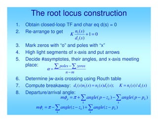
1. The root locus construction
1. Obtain closed-loop TF and char eq d(s) = 0
2. Re-arrange to get
3. Mark zeros with “o” and poles with “x”
4. High light segments of x-axis and put arrows
5. Decide #asymptotes, their angles, and x-axis meeting
place:
6. Determine jw-axis crossing using Routh table
7. Compute breakaway:
8. Departure/arrival angle:
0
1
)
(
)
(
1
1
=
+
s
d
s
n
K
m
n
zeros
poles
−
−
=


α
)
(
/
)
(
);
(
)
(
)
(
)
( 1
1
'
1
1
'
1
1 s
d
s
n
K
s
d
s
n
s
n
s
d =
=

 −
−
−
+
=
k
k
k
k
p p
p
angle
z
p
angle
m )
(
)
(
π
φ

 −
+
−
−
=
k
k
k
k
z p
z
angle
z
z
angle
m )
(
)
(
π
φ

2. General controller design
G(s)
C(s)
+
-
r(s) e y(s)
plant
controller
Goal: for a given plant G(s)
a set of desired step response specifications
design a controller C(s) such that
the closed-loop step response meets the desired specs

3. RL based controller parameter selection
• Controller form is given
• A single parameter needs to be determined
– Draw root locus
– Select dominant poles in the desired region
• Two parameter needs to be determined
– Use required specification to reduce degree of
freedoms to one
– Draw root locus
– Select dominant pole in desired region

4. Effects of additional pole
• One additional R.L. branch shoots out
• It increases # asymp. by one
– More asymptotes go towards +Re-axis
– More likely to be unstable
• Poles tend to push R.L. away from them
Don’t introduce poles unless required by
other concerns

5. Examples:
2
asymp
# =

6. Effects of additional zero
• It sinks one branch of R.L.
• It reduces the # asymp. by one
– Asymptotes move more towards –Re-axis
– More likely to be stable
• Zeros attract R.L.
– Each zero attracts one branch
– If > 1 branches nearby, they go to Re-axis
& split, the one branch goes to zero
– Never have >= 2 branches go to a zero

7. Examples:

8. • The dominant pole
pair are more
negative
• But there is one pole
(real) close to s = 0,
which will settle very
slowly (sluggish
settling)
If we put that additional zero
near (0,0):

9. Controller design by R.L.
Typical setup:
C(s) G(s)
( )
( )
( )
( )
0
1
1
1
=
+
⋅
−
−
s
d
s
n
p
s
z
s
K
L
L
( ) ( )
( )
s
d
s
n
s
G =
( )( )
( )( )L
L
2
1
2
1
)
(
p
s
p
s
z
s
z
s
K
s
C
−
−
−
−
=
Controller Design Goal:
1. Select poles and zero of C(s) so that R.L. pass through desired region
2. Select K corresponding to a good choice of dominant pole pair

10. Matlab program template
% enter plant transfer function Gp(s)
nump = …. ; denp=…. ;
% enter desired closed loop step response specification:
% you may allow both uppper and lower limits
… …
% convert from specs to zeta, omegan, sigma, omegad
… …
%Draw root locus; may need to re-arrange equation based on steady state ess requirements
…
%adjust window size, x-limit, y-limit, etc using values of omegan, sigma, omegad
…
% hold the graph, and plot allowable region for pole location on RL graph
… …
% Computer controller transfer function
%if PD or lead needed, design a PD or lead
…
%if PI or lag needed, design a PI or lag
…
%design P, or final decision on overall gain
…
% get controller TF
…
% obtain closed loop transfer function from Gp(s) and C(s)
… … numcl=…; dencl=…; … …
% obtain closed-loop step response
… …
% compute actual step response specs, using your program from before
… …
% are they good?
% compute the actual closed-loop poles, place “x” at those locations
… …
% are they in the allowable region?

11. Proportional control design
1. Draw R.L. for given plant
2. Draw desired region for poles from specs
3. Pick a point on R.L. and in desired region
• Use ginput to get point and convert to complex #
4. Compute K using abs
and polyval
5. Obtain closed-loop TF
6. Obtain step response and compute specs
7. Decide if modification is needed
( )
( )
0
1=
+
s
d
s
n
K
( ) ( )
D
P
G
s
G
K
1
1
=
−
=

12. When to use:
If R.L. of G(s) goes through
the desired region for c.l. poles
What is that region:
– From design specs, get desired Mp, ts, tr,
etc.
– Use formulae for 2nd order system to get
desired ωn , ζ, σ, ωd
– Identify / plot these in s-plane

13. Example:
When C(s) = 1, things are okay
But we want initial response speed as fast as
possible; yet we can only tolerate 10%
overshoot.
Sol: From the above, we need
that means:
( )
6
1
+
s
s
%
10
≤
p
M
6
.
0
≥
ζ
C(s)

21. This is a cone around –Re axis with ±60° area
We also want tr to be as small as possible.
i.e. : want ωn as large as possible
i.e. : want pd to be as far away from s = 0 as
possible
1. Enter plant, Draw R.L., draw max Mp cone
2. Since RL pass through desired cone, Pick
pd on R.L., in cone, with max | pd |
3.
( )
25
6
1
=
+
⋅
=
= d
d
d
p
p
p
G
K

22. Root Locus
Real Axis
Imaginary
Axis
-7 -6 -5 -4 -3 -2 -1 0 1
-5
-4
-3
-2
-1
0
1
2
3
4
5
System: sys
Gain: 24.9
Pole: -3 - 3.99i
Damping: 0.601
Overshoot (%): 9.43
Frequency (rad/sec): 4.99
n=1; d=[1 6 0]; sys_p = tf(n,d);
rlocus(sys_p);
[x,y]=ginput(1); pd=x+j*y;
Gpd = evalfr(sys_p, pd); K=1/abs(Gpd);



 K=25

23. 0 0.2 0.4 0.6 0.8 1 1.2 1.4 1.6
0
0.2
0.4
0.6
0.8
1
1.2
1.4
System: sys
Time (sec): 0.79
Amplitude: 1.09
Step Response
Time (sec)
Amplitude
sys_cl = feedback(K*sys_p,1);
mystep(sys_cl);

24. Example:
Want: , as fast as possible
Sol:
1. Draw R.L. for
2.
Draw cone ±45° about –Re axis
3. Pick pd as the crossing point of the
ζ= 0.7 line & R.L.
4.
( )
( )( )
6
2
10
+
+
=
s
s
s
s
G
%
5
≤
p
M
( )
1
2 6 10 0.94
P d d d
d
K p p p
G p
= = ⋅ + ⋅ + ≈
7
.
0
%
5 ≥

≤ ζ
p
M
( )
6
)
2
(
10
+
+ s
s
s
C(s)
pd=-0.9+j0.9

25. -25 -20 -15 -10 -5 0 5 10
-20
-15
-10
-5
0
5
10
15
20
Root Locus
Real Axis
Im
a
g
in
a
r
y
A
x
is

26. 0 1 2 3 4 5 6 7 8
0
0.2
0.4
0.6
0.8
1
Step Response
Time (sec)
Amplitude
Overshoot is a little too much.
Re-choose pd =-0.8+j0.8

28. -6 -5 -4 -3 -2 -1 0 1
-5
0
5
0.12
0.24
0.38
0.5
0.64
0.76
0.88
0.97
0.12
0.24
0.38
0.5
0.64
0.76
0.88
0.97
1
2
3
4
5
6
Root Locus
RealAxis
I
m
a
g
i
n
a
r
y
A
x
i
s

29. ylim([0,yss*(1+Mp)])
0 1 2 3 4 5 6 7
0
0.2
0.4
0.6
0.8
1
Step Response
Time (sec)
Amplitude

30. Controller tuning:
1. First design typically may not work
2. Identify trends of specs changes as K
is increased.
e.g.: as KP , pole
3. Perform closed-loop step response
4. Adjust K to improve specs
e.g. If MP too much, the 2. says
reduce KP
↑
↓
∴
↑
↓
∴ P
d M
&
,
, ζ
ω
σ

31. PD controller design
•
• This is introducing an additional zero to
the R.L. for G(s)
• Use this if the dominant pole pair
branches of G(s) do not pass through
the desired region
• Place additional zero to “bend” the RL
into the desired region
( ) ( )
z
s
K
s
K
K
s
C D
D
P +
=
+
=
D
P K
K
z =

33. Design steps:
1. From specs, draw desired region for pole.
Pick from region, not on RL
2. Compute
3. Select
4. Select:
d
d j
p ω
σ +
−
=
( )
d
p
G
∠
( ) ( )
d
d p
G
z
p
z ∠
−
=
+
∠ π
s.t.
( )
( )
d
d p
G
z ∠
−
+
= π
ω
σ tan
i.e.
( )





⋅
=
⋅
+
=
D
P
d
d
D
K
z
K
p
G
z
p
K
1
Gpd=evalfr(sys_p,pd)
phi=pi - angle(Gpd)
z=abs(real(pd))+abs(imag(pd)/tan(phi))
Kd=1/abs(pd+z)/abs(Gpd)
Use [x, y] = ginput(1);
pd = x+j*y;

36. Example:
Want:
Sol:
(pd not on R.L.)
(Need a zero to attract R.L. to pd)
%
2
sec
2
%,
5 for
t
M s
p ≤
≤
7
.
0
%
5 ≥

≤ ζ
p
M
2
4
sec
2 ≥
=

≤
s
s
t
t σ
2
2
Choose j
pd +
−
=
( )
707
.
0
,
2
,
2 =
=
= ζ
ω
σ d
)
2
(
1
+
s
s
C(s)

41. 2.
3.
4.
( )
4
tan π
ω
σ d
z +
=
( ) ( )( )
2
2
2
2
2
1
+
+
−
+
−
∠
=
∠ j
j
d
p
G
( ) 2
2
2 j
j ∠
−
+
−
−∠
=
4
3
4
5
2
4
3 π
π
π
π
=
−
=
−
−
=
4
1
2
2 =
+
=
( )( )





=
⋅
=
=
+
+
−
⋅
+
−
+
+
−
= −
8
2
2
2
2
2
2
4
2
2
1
1
D
P
D
K
z
K
j
j
j
K
( ) s
s
C 2
8+
=
( ) 4
4
3 π
π
π
π =
−
=
∠
− d
p
G

42. 0 0.5 1 1.5 2 2.5 3
0
0.2
0.4
0.6
0.8
1
Step Response
Time (sec)
Amplitude
ts is OK
But Mp too large
To redesign:
Reduce ωd
pd=-2+j1.5

43. Gpd = evalfr(sys_p, pd)
Gpd = - 0.1600 + 0.2133i
phi = pi - angle(Gpd)
phi = 0.9273
z = abs(real(pd)) + abs(imag(pd)/tan( phi))
z = 3.1250
Kd = 1/abs(pd+z)/abs(Gpd)
Kd = 2
Kp = z*Kd
Kp = 6.2500
sys_c=tf([Kd Kp], 1);
sys_cl=feedback(sys_c*sys_p, 1)
Transfer function:
2 s + 6.25
----------------
s^2 + 4 s + 6.25
step(sys_cl); ylim([0 yss*(1+2*Mp)])

44. 0 0.5 1 1.5 2 2.5 3
0
0.2
0.4
0.6
0.8
1
Step Response
Time (sec)
Amplitude

45. Drawbacks of PD
• Not proper : deg of num > deg of den
• High frequency gain → ∞:
• High gain for noise since noise is HF
Saturates circuits
Cannot be implemented physically
as
P D
K K jω ω
+ → ∞ → ∞
Q

∴


46. Lead Controller
• Approximation to PD
• Same usefulness as PD
•
• It contributes a lead angle:
( ) 0
>
>
+
+
= z
p
p
s
z
s
K
s
C
( ) ( )
z
p
p
C d
d +
∠
=
∠
φ
=
( )
p
pd +
∠
−

47. Lead Design:
1. Enter G, Draw R.L. for G
2. Enter specs, draw region for desired c.l.
poles
3. Select pd from region
4. Let
Pick –z somewhere below pd on –Re axis
Let
Select
( )
d
d j
p ω
σ +
−
=
( )
d
p
G
∠
−
= π
φ
( ) φ
φ
φ
φ −
=
+
∠
= 1
2
1 ,
z
pd
( ) 2
s.t. φ
=
+
∠ p
p
p d
( )
2
tan
i.e. φ
ω
σ d
p +
=
C(s) G(s)

48. • There are many choices of z, p
• More neg. (–z) & (–p) → more close to
PD & more sensitive to noise, and
worse steady-state error
• But if –z is > Re(pd), pd may not
dominate
( ) ( )
d
d
d
d
p
d
p
z
d
p p
G
z
p
p
p
p
G
K
⋅
+
+
=
⋅
=
+
+
1
Let
( )
p
s
z
s
K
s
C
+
+
=
:
is
controller
Your

49. Example: Lead Design
MP is fine,
but too slow.
Want: Don’t increase MP
but double the resp. speed
Sol: Original system: C(s) = 1
Since MP is a function of ζ, speed is
proportional to ωn
5
.
0
2
2
,
2 =

=
= ζ
ζω
ω n
n
4
2
2
4
TF
c.l.
+
+
=
s
s
C(s)
)
2
(
4
+
s
s

51. Draw R.L. & desired
region
Pick pd right at the
vertex:
(Could pick pd a little
inside the region
to allow “flex”)
5
.
0
new
want
we
Hence ≥
ζ
4
new ≥
n
ω
3
2
2 j
pd +
−
=

53. Clearly, R.L. does not pass through pd,
nor the desired region.
need PD or Lead to “bend” the R.L.
into region.
(Note our choice may be the easiest to
achieve)
Let’s do Lead:
( ) ( )
2
+
∠
+
∠
+
=
−
= d
d
d p
p
p
G π
π
φ
∴
6
2
3
2 π
π
π
π =
+
+
=

54. Pick –z to the left of pd
4
,
4
Pick =
−
=
− z
z
( )
3
4
1
π
φ =
+
∠
= d
p
6
6
3
then 1
2
π
π
π
φ
φ
φ =
−
=
−
=
( )
2
tan
then φ
ω
σ d
p +
=
8
3
2
2 3
1
=
+
=
( )
7
2
4
1
≈
=
+
⋅
+
+
d
p
d
p
p
d
p
z
d
p
K
( ) 8
4
7 +
+
=
∴ s
s
s
C

55. 0 0.5 1 1.5 2 2.5 3
0
0.2
0.4
0.6
0.8
1
1.2
Step Response
Time (sec)
Amplitude
Speed is doubled, but over shoot is too much.

56. 0 0.5 1 1.5 2 2.5 3
0
0.2
0.4
0.6
0.8
1
1.2
Step Response
Time (sec)
Amplitude
( )
8
4
7
+
+
=
s
s
s
C ( )
10
4
6
+
+
=
s
s
s
C
Change controller from to
To reduce the gain a bit, and make it a little closer to PD

57. Particular choice of z :
( ) ( ) ( )
2
2
2
1
φ
φ
φ +
∠
=
+
∠
=
−
∠
=
−
∠
=
+
∠
= d
d
d
d
d
p
A
Bp
A
p
z
p
z
O
z
p
( )=
+
∠
= p
pd
2
φ
( )
∞
+
∠
=
∠ O
p
O
Ap d
d d
p
∠
=
O
Ap
Bp d
d ∠
bisect
s.t.
B
Choose
A
Bp
OBp d
d ∠
=
∠
∴
O
Apd
∠
= 2
1
d
p
∠
= 2
1
2
2
φ
−
∠
= d
p

58. ( )
1
tan φ
ω
σ d
z +
=
( )
2
tan φ
ω
σ d
p +
=
3
2
2
:
example
prev.
In j
pd +
−
=
3
2
,
2 =
= d
ω
σ
get
we
procedure,
above
Follow
( ) 46
.
5
93
.
2
73
.
4 +
+
= s
s
s
C
359
.
0
,
%
21
:
step
c.l. =
= r
p t
M
repeat.
,
5
.
2
to
2
change =
σ
375
.
0
,
%
1
.
16
:
step
c.l. =
= r
p t
M