1. Solution
Week 60 (11/3/03)
Cereal box prizes
First Solution: Assume that you have collected c of the colors, and let Bc be the
number of boxes it takes to get the next color. The average value of Bc, which we
will denote by Bc, may be found as follows. The probability that a box yields a new
color is 1 − c/N, and the probability that it does not is c/N. The expected number
of boxes to get the next prize is therefore
Bc = 1 1 −
c
N
+ 2
c
N
1 −
c
N
+ 3
c
N
2
1 −
c
N
+ · · · . (1)
Letting x ≡ c/N, we have
Bc = (1 − x)(1 + 2x + 3x2
+ 4x3
+ · · ·)
= (1 − x) (1 + x + x2
+ · · ·) + (x + x2
+ · · ·) + (x2
+ · · ·) + · · ·
= (1 − x)
1
1 − x
+
x
1 − x
+
x2
1 − x
+ · · ·
=
1
1 − x
. (2)
Therefore,
Bc =
N
N − c
. (3)
Note that the above 1 + 2x + 3x2 + · · · = 1/(1 − x)2 result, for 0 ≤ x < 1, may also
be derived by taking the derivative of the equality 1 + x + x2 + · · · = 1/(1 − x).
We see that (with c = 0) it takes one box, of course, to get the first color. Then
(with c = 1) it takes an average of N/(N − 1) boxes to get the second color. Then
(with c = 2) it takes an average of N/(N − 2) boxes to get the third color. This
continues until (with c = N −1) it takes an average of N boxes to get the last color.
We wish to find the average, B, of the total number of boxes needed to get all the
colors. B can be viewed as the average of the sum of the waiting times for each new
color. But this equals the sum of the average waiting times, which were calculated
above. In other words, letting B be the total number of boxes in a particular trial,
and letting B0, B1, . . . , BN−1 be the waiting times during that particular trial, we
have (with a bar denoting average)
B = (B0 + B1 + · · · + BN−1)
= B0 + B1 + · · · + BN−1
= N
1
N
+
1
N − 1
+ · · · +
1
2
+ 1 . (4)
For large N, this goes like
B ≈ N(ln N + γ), (5)
where γ ≈ 0.577 is Euler’s constant.
1

2. Second Solution: We will calculate the probability, P(n), that the final color is
obtained in the nth box. The desired expectation value is then ∞
0 nP(n).
Claim: P(n) =
N−1
k=1
(−1)k−1 N − 1
k − 1
1 −
k
N
n−1
(n = 2, 3, . . .).
Proof: Let us first calculate the probability, p(n), that you have obtained all
the colors by the time you have looked in the nth box. P(n) is then given by
P(n) = p(n) − p(n − 1).
Assume that n boxes have been bought. Then there is a total of Nn equally
likely possibilities for the way the colors can turn up in these n boxes. In finding
p(n), we will need to subtract from Nn the number of possibilities that do not have
at least one prize of each color. We can count this number is the following way.
If (at least) color 1 is missing, then there are (N − 1)n different combinations.
Likewise for the situations where another color is missing. So there seem to be
N(N − 1)n combinations missing a color. However, we have double-counted some
of the cases. For example, a combination which has (at least) 1 and 2 missing has
been counted twice; there are (N − 2)n of these. Likewise for all the other pairs of
colors. So we must subtract off N
2 (N − 2)n combinations. But now a combination
which has (at least) 1, 2, and 3 missing has not been counted at all (because we have
included it three times, and then subtracted it off three times); there are (N −3)n of
these. Likewise for the other triplets. So we must add on N
3 (N −3)n combinations.
Now, however, the combinations with (at least) 1, 2, 3, and 4 missing have been
counted 4
1 − 4
2 + 4
3 = 2 times. Likewise for the other quadruplets. So we must
subtract off N
4 (N − 4)n combinations.
In general, if we have done this procedure up to (k − 1)-tuplets, then the com-
binations missing (at least) k of the colors have been counted T times, where
T =
k
1
−
k
2
+ · · · + (−1)k k
k − 1
. (6)
However, the binomial expansion gives
0 = (1 − 1)k
= 1 −
k
1
+
k
2
+ · · · + (−1)k−1 k
k − 1
+ (−1)k
= 1 − T + (−1)k
. (7)
Therefore, T = 2 for even k, and T = 0 for odd k. So we have either overcounted
by one, or undercounted by one. Hence, the total number of combinations missing
at least one color is
N
1
(N − 1)n
−
N
2
(N − 2)n
+ · · · + (−1)N N
N − 1
(1)n
. (8)
To obtain the probability, p(n), that you have collected all the colors by the nth
box, we must subtract this number from Nn, and then divide the result by Nn. We
2

3. obtain
p(n) =
N−1
k=0
(−1)k N
k
1 −
k
N
n
, (n = 1, 2, 3, . . .). (9)
Remark: p(n) must of course equal zero, for n = 1, 2, . . . , N − 1, because you need to buy
at least N boxes to get all the colors. To show this explicitly, first note that p(n) may be
written as
p(n) =
N
k=0
(−1)k N
k
1 −
k
N
n
, (10)
where we have let the sum run up to k = N, because the k = N term is zero anyway. It
is therefore sufficient to demonstrate that
N
k=0 (−1)k N
k km
= 0, for m = 0, 1, . . . N − 1,
because this identity will make all the separate terms arising from the binomial expansion
of (1 − k/N)n
in eq. (10) equal to zero on their own. You can prove this identity by taking
successive derivatives of the relation (1 − x)N
= (−1)k N
k xk
, and setting x = 1.
The probability, P(n), that the final color is obtained in the nth box is
P(n) = p(n) − p(n − 1)
=
N−1
k=0
(−1)k N
k
1 −
k
N
n−1
1 −
k
N
− 1
=
N−1
k=0
(−1)k N!
k!(N − k)!
1 −
k
N
n−1
−
k
N
=
N−1
k=1
(−1)k−1 N − 1
k − 1
1 −
k
N
n−1
, (n = 2, 3, . . .). (11)
P(n) is zero for n = 2, 3, . . . , N − 1. And P(1) is of course also zero, but it cannot
be expressed as in eq. (11), because eq. (9) is not valid for n = 0.
Having found P(n), we can write the average number, B, of required boxes as
B =
∞
n=2
n
N−1
k=1
(−1)k−1 N − 1
k − 1
1 −
k
N
n−1
. (12)
We have let the sum over n range from 2 to ∞, instead of N to ∞, because it will
simplify our calculations a bit (and all the terms from n = 2 to n = N − 1 are
zero). Switching the order of the sums, and performing the sum over n by using a
technique similar to the one used in eq. (2), we obtain
B =
N−1
k=1
(−1)k−1 N − 1
k − 1
N2
k2
− 1
=
N−1
k=1
(−1)k−1 (N − 1)!
(k − 1)!(N − k)!
(N + k)(N − k)
k2
= −
N−1
k=1
(−1)k N − 1
k
1 +
N
k
3

4. = −
N−1
k=1
(−1)k N − 1
k
−
N−1
k=1
(−1)k N − 1
k
N
k
= − (1 − 1)N−1
− 1 − N
N−1
k=1
(−1)k N − 1
k
1
k
.
= 1 − N
N−1
k=1
(−1)k N − 1
k
1
k
. (13)
At this point, we need the following claim.
Claim:
M
k=1
(−1)k M
k
1
k
= − 1 +
1
2
+
1
3
+ · · · +
1
M
.
Proof: We will prove this by using a technique similar to the one mentioned in the
above Remark, except that now we will find it necessary to take an integral instead
of a derivative, because we want to produce a k in the denominator. Starting with
the binomial expansion, we have
M
k=0
(−1)k M
k
xk
= (1 − x)M
(14)
=⇒
M
k=1
(−1)k M
k
xk−1
dx =
1
x
(1 − x)M
− 1 dx
=⇒
M
k=1
(−1)k M
k
xk
k
= −
1 − (1 − x)M
1 − (1 − x)
dx
=⇒
M
k=1
(−1)k M
k
xk
k
= − 1 + (1 − x) + · · · + (1 − x)M−1
dx
=⇒
M
k=1
(−1)k M
k
xk
k
= (1 − x) +
1
2
(1 − x)2
+ · · · +
1
M
(1 − x)M
+ C,
where C is a constant of integration. Setting x = 0 in the last line yields
C = − 1 +
1
2
+
1
3
+ · · · +
1
M
. (15)
Setting x = 1 in the last line then proves the claim.
Using the claim in eq. (13) gives
B = 1 + N
1
N − 1
+ · · · +
1
2
+ 1
= N
1
N
+
1
N − 1
+ · · · +
1
2
+ 1 , (16)
in agreement with eq. (4).
4

5. Now let us maximize P(n), as given in eq. (11). For convenience, we will instead
maximize P(n + 1), so that there will be a simpler “n” in the exponent in eq. (11),
instead of “n − 1”. Of course, such a distinction is irrelevant in the limit of large N.
Let us assume for the moment (we will justify this below) that the values of k that
contribute significantly to the sum in eq. (11) are small enough so that we may use
the approximation,
1 −
k
N
n
≈ e−n/N
k
. (17)
The expression for P(n + 1) in eq. (11) then becomes (letting the sum run up to
k = N, since the k = N term is zero)
P(n + 1) ≈ e−n/N
N
k=1
(−1)k−1 N − 1
k − 1
e−n/N
k−1
= e−n/N
N−1
j=0
(−1)j N − 1
j
e−n/N
j
= e−n/N
1 − e−n/N
N−1
≈ e−n/N
e−(N−1)e−n/N
. (18)
To maximize P(n), we therefore want to minimize n/N +(N −1)e−n/N . Taking the
derivative of this with respect to n, we find that the minimum is achieved when
nmax = N ln(N − 1) ≈ N ln N, (19)
where we have dropped terms of order 1. Using this result in eq. (18), we see that
the maximum value of P(n), which is obtained at n ≈ N ln N, equals 1/(Ne).
Remarks:
1. Let us now justify eq. (17). Using
ln 1 −
k
N
n
= n ln 1 −
k
N
≈ n −
k
N
−
k2
2N2
− · · · , (20)
we have
1 −
k
N
n
≈ e−nk/N
e−nk2/2N2
. (21)
Therefore, eq. (17) is valid if nk2/N2 1. For n near N ln N, which is the
general size of n we are concerned with, this requires that k N/ ln N.
But for large N and for n ≈ N ln N, the first few terms in the second (and
hence first) line of eq. (18) dominate the sum. This is true because the
binomial coefficient goes like Nj/j!, and the (e−n/N )j term goes like 1/Nj
(using n ≈ N ln N). Hence, the the jth term goes like 1/j!. Therefore, only
the first few terms contribute, so the relevant k values easily satisfy the bound
k N/ ln N.
Note also that the step in going from the third to fourth line in eq. (18) is
valid because e−n/N ≈ 1/N is sufficiently small.
5

6. 2. For large N, the average number of boxes, and the point where P(n) is maxi-
mum (given in eqs. (5) and (19), respectively) are
B = N(ln N + γ) and nmax = N ln N. (22)
The difference between these is γN ≈ (0.577)N. For example, when N = 100,
the maximum occurs at N ln N ≈ 460, while the average number is N ln N +
γN ≈ 518.
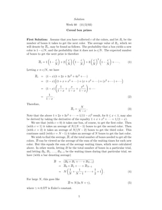
3. If we let n ≡ N ln N + xN, then we can rewrite eq. (18), to leading order in
N, as
NP(x) ≈ e−x−e−x
. (23)
A plot of NP(x) vs. x is shown below. This is simply a plot of NP(n) vs. n,
centered at N ln N, and with the horizontal axis on a scale of N.
x
NP(x)
NP(γ) = 0.32
1-1 20-2 3
0.1
0.2
0.3
NP(0) = 1/e = 0.37
-x-e-x
e
γ
For all large N, we obtain the same shape. Virtually all of the graph is
contained within a few units of N from the maximum. Compared to a P(n)
vs. n graph, this graph has its vertical axis multiplied by N and its horizontal
axis multiplied by 1/N, so the total integral should still be 1. And indeed,
∞
−∞
e−x−e−x
dx = e−e−x ∞
−∞
= 1. (24)
How much area under the curve lies to the left of, say, x = −2? Letting
x = −a to be general, the integral in eq. (24) gives an area (in other words,
a probability) of e−e−x
|−a
−∞ = e−ea
. This decreases very rapidly as a grows.
Even for a = 2, we find that there is a probability of only 0.06% of obtaining
all the colors before you hit the n = N ln N − 2N box.
How much area under the curve lies to the right of, say, x = 3? Letting x = b
to be general, we find an area of e−e−x
|∞
b = 1 − e−e−b
≈ 1 − (1 − e−b) = e−b.
This decreases as b grows, but not as rapidly as in the above case. For b = 3,
we find that there is a probability of 5% that you haven’t obtained all the
colors by the time you hit the n = N ln N + 3N box.
6

7. 4. You might be tempted to fiddle around with a saddle-point approximation in
this problem. That is, you might want to approximate P(n) as a Gaussian
around its maximum at nmax ≈ N ln N. However, this will not work in this
problem, because for any (large) N, P(n) will always keep its same lopsided
shape. The average will always be a significant distance (namely γN, which
is comparable to the spread of the graph) from the maximum, and the ratio
of the height at the average to the height at the maximum will always be
P(γ)
P(0)
=
e−γ−e−γ
e−0−e−0 ≈ 0.87. (25)
7