Rectangular Coordinates in Three Dimensions

11.2 Rectangular Coordinates in Three Dimensions Contemporary Calculus 1

11.2 RECTANGULAR COORDINATES IN THREE DIMENSIONS

In this section we move into 3–dimensional space. First we examine the 3–dimensional rectangular
coordinate system, how to locate points in three dimensions, distance between points in three dimensions,
and the graphs of some simple 3–dimensional objects. Then, as we did in two dimensions, we discuss
vectors in three dimensions, the basic properties and techniques with 3–dimensional vectors, and some of
their applications. The extension of the algebraic representations and techniques from 2 to three dimensions
is straightforward, but it usually takes practice to visualize 3–dimensional objects and to sketch them on a
2–dimensional piece of paper.

3–Dimensional Rectangular Coordinate System (x, y
y

In the 2–dimensional rectangular coordinate system we have two coordinate axes that meet
at right angles at the origin (Fig. 1), and it takes two numbers, an ordered pair (x, y), to x
Fig. 1
specify the rectangular coordinate location of a point in the plane (2 dimensions). Each
ordered pair (x, y) specifies the location of exactly one point, and the
location of each point is given by exactly one ordered pair (x, y). positive
z–axis
The x and y values are the coordinates of the point (x, y). point
(x, y, z) z
3 right angles
The situation in three dimensions is very similar. In the
3–dimensional rectangular coordinate system we have three coordinate
axes that meet at right angles (Fig. 2), and three numbers, an ordered y
x
triple (x, y, z), are needed to specify the location of a point. Each
ordered triple (x, y, z) specifies the location of exactly one point, positive positive
x–axis y–axis
and the location of each point is given by exactly one ordered triple Fig. 2
(x, y, z). The x, y and z values are the coordinates of the
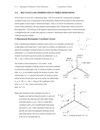
point (x, y, z). Fig. 3 shows the location of the z
4
point (4, 2, 3).
3
(0, 2, 3)
Right–hand orientation of the coordinate axes (Fig. 4): 2
(4, 0, 3)
Imagine your right arm along the positive x–axis with 1
your hand at the origin and your index finger curling
(4, 2, 3) 1 1
toward the positive y–axis. Then, in a right–hand
2 2
coordinate system, your extended thumb points along 3 3
4 4
the positive z–axis. Other orientations of the axes are
x y
possible and valid (with appropriate labeling), but the
(4, 2, 0)
right–hand system is the most common orientation and
Fig. 3: Locating the point (4, 2, 3)
is the one we will generally use.


The three coordinate axes determine three planes (Fig.5): the
xy–plane consisting of all points with z–coordinate 0, the thumb negative
x–axis
xz–plane consisting of all points with y–coordinate 0, and the
yz–plane with x–coordinate 0. These three planes then divide the
3–dimensional space into 8 pieces called octants. The only
octant we shall refer to by name is the first octant which is the
octant determined by the positive x, y, and z–axes (Fig. 6).
Fig. 4: Right–hand coordinate system

positive
z–axis

The collection
of points in the
(infinite) box is
called the first
octant: x ≥ 0,
x
y ≥ 0, z ≥ 0

positive positive
x–axis y–axis
Fig. 5: Coordinate Planes
Fig. 6

Visualization in three dimensions: Some people have difficulty visualizing points and other objects in
three dimensions, and it may be useful for you to spend a few minutes to create a small model of
the 3–dimensional axis system for your desk. One model consists of a corner of a box (or room)
as in Fig. 7: the floor is the xy–plane; the wall with the window is the xz–plane; and the wall
with the door is the yz–plane. Another simple model uses a small Styrofoam ball and three
pencils (Fig. 8): just stick the pencils into the ball as in Fig. 8, label each pencil as the
appropriate axis, and mark a
z few units along each axis z
(pencil). By referring to
such a model for your early
work in three dimensions, it
becomes easier to visualize
the locations of points and
the shapes of other objects
x Fig. 8 y
x y later. This visualization

Fig. 7 can be very helpful.


Each ordered triple (x, y, z) specifies the location of a single point, and this z–axis
location point can be plotted by locating the point (x, y, 0) on the
point
xy–plane and then going up z units (Fig. 9). (We could also get to the (x, y, z) z
same (x, y, z) point by finding the point (x, 0, z) on the xz–plane and (0, y, z)

then going y units parallel to the y–axis, or by finding (0, y, z) on the (x, 0, z)

yz–plane and then going x units parallel to the x–axis.) y
x
Example 1: Plot the locations of the points P = (0, 3, 4), Q = (2, 0, 4), y–axis
x–axis (x, y, 0)
R = (1, 4, 0), S = (3, 2, 1), and T(–1, 2, 1) .
Fig. 9

Solution: The points are shown in Fig. 10. z
4
Q(2, 0, 4)
Practice 1: Plot and label the locations of the points 3
P(0, 3, 4)
A = (0, –2, 3), B = (1, 0, –5), C = (–1, 3, 0), and
2
D = (1, –2, 3) on the coordinate system in Fig. 11.
1
T(–1, 2, 1)
1 1
4
z
2 2
3 S(3, 2, 1) 3
3 4 4
x y
2 R(1, 4, 0)
1 Fig. 10

1 1
2 Practice 2: The opposite corners of a rectangular
2
3 3 box are at (0, 1, 2) and (2, 4, 3).
4 4
x Sketch the box and find its volume.
y

Fig. 11
4
z

Once we can locate points, we can begin to consider the graphs 3
of various collections of points. By the graph of "z = 2" we
2
mean the collection of all points (x, y, z) which have the form
1
"(x, y, 2)". Since no condition is imposed on the x and y
variables, they take all possible values. The graph of z = 2 1 1
(Fig. 12) is a plane parallel to the xy–plane and 2 units above 2 2
3 3
the xy–plane. Similarly, the graph of y = 3 is a plane parallel 4 4
to the xz–plane (Fig. 13a), and x = 4 is a plane parallel to the x y
yz–plane (Fig. 13b).
Fig. 12: Plane z = 2


Plane Plane
y = 3 x = 4

1
1

(a)
(b)
Fig. 13: Planes y = 3 and x = 4

Practice 3: Graph the planes (a) x = 2, (b) y = –1, and 4
z

(c) z = 3 in Fig. 14. Give the coordinates of
3
the point that lies on all three planes.
2
Example 2: Graph the set of points (x, y, z) such that
1
x = 2 and y = 3.
1 1
Solution: The points that satisfy the conditions all have the 2 2
3 3
form (2, 3, z), and, since no restriction has been placed on 4 4
the z–variable, z takes all values. The result is the line x y
(Fig. 15) through the point (2, 3, 0) and parallel to the
Fig. 14
z–axis.

4
z

Practice 4: On Fig. 15, graph the points that have the
3
form (a) (x, 1, 4) and (b) (2, y, –1).
2

1
In Section 11.5 we will examine planes and lines that are

1 not parallel to any of the coordinate planes or axes.
1
2 2
3 3
4 4 Example 3: Graph the set of points (x, y, z) such that
x y x2 + z2 = 1.
(2, 3, 0)

line (2, 3, z)
Fig. 15


Solution: In the xz–plane (y = 0), the graph of x2 + z2 = 1 is a circle centered at the origin and with
radius 1 (Fig. 16a). Since no restriction has been placed on the y–variable, y takes all values.
The result is the cylinder in Figs. 16b and 16c, a circle moved parallel to the y–axis.

z z z
x 2 + z2 = 1 x 2 + z2 = 1
x 2 + z2 = 1 no restriction on y
y=0
1 1 1 cylinder
cylinder
circle
–1 –1

1 1 1

x y x y x y
–1 –1 –1
(a) (b) (c)
Fig. 16

Practice 5: Graph the set of points (x, y, z) such that y2 + z2 = 4. (Suggestion: First graph
y2 + z2 = 4 in the yz–plane, x = 0, and then extend the result as x takes on all values.)

Distance Between Points
Two dimensions
y
In two dimensions we can think of the distance between points as the length Q
e
anc
of the hypotenuse of a right triangle (Fig. 17), and that leads to the dist ∆y
2 2
Pythagorean formula: distance = ∆x + ∆y . In three dimensions P ∆x
x
we can also think of the distance between points as the length of the
Fig. 17
hypotenuse of a right triangle (Fig. 18), but in this situation the calculations
appear more complicated. Fortunately, they are straightforward:

Three dimensions distance2 = base2 + height2 = ( ∆x 2 + ∆y 2 ) 2 + ∆z2
z
= ∆x2 + ∆y2 + ∆z2 so distance = ∆x2 + ∆y2 + ∆z2 .

If P = (x1 , y1 , z1 ) and Q = (x2 , y2 , z2 ) are points in space,
Q
e
anc then the distance between P and Q is
dist ∆z

x y distance = ∆x 2 + ∆y 2 + ∆z 2
P base
∆y ∆x 2 2 2
= (x 2 –x 1 ) + (y 2 –y 1 ) + (z 2 –z 1 ) .
Fig. 18

The 3–dimensional pattern is very similar to the 2–dimensional pattern with the additional piece ∆z2 .


Example 4: Find the distances between all of the pairs of the given points. Do any three of these points
form a right triangle? Do any three of these points lie on a straight line?
Points: A = (1, 2, 3), B = (7, 5, –3), C = (8, 7, –1), D = (11, 13, 5) .

Solution: Dist(A, B) = 6 2 + 3 2 + (–6) 2 = 36 + 9 + 36 = 81 = 9. Similarly,

Dist(A,C) = 90 , Dist(A, D) = 15, Dist(B, C) = 3, Dist(B, D) = 12, and Dist(C, D) = 9.

{ Dist(A, B) }2 + { Dist(B, D) }2 = { Dist(A, D) }2 so the points A, B, and D form a right
triangle with the right angle at point B. Also, the points A, B, and C form a right triangle
with the right angle at point B since 92 + 32 = ( 90 )2

Dist(B, C) + Dist(C, D) = Dist(B, D) so the points
z
B, C, and D line on a straight line. The points are shown in 5
Fig. 19. In three dimensions it is often difficult to determine A
the size of an angle from a graph or to determine whether points
5 5
are collinear.
10 10
x
Practice 6: Find the distances between all of the pairs of the D y
B C
given points. Which pair are closest together? Which pair
are farthest apart? Do the three points form a right triangle? Fig. 19
Points: A = (3, 1, 2), B = (9, 7, 5), C = (9, 7, 9) .
y (x–2) 2 + (y–3) 2 = 5 2
8

In two dimensions, the set of points at a fixed distance from a given point
5
is a circle, and we used the distance formula to determine equations
3
describing circles: the circle with center (2, 3) and radius 5 (Fig. 20) is
x
given by (x–2)2 + (y–3)2 = 52 or x2 + y2 – 4x – 6y = 12.
2 7
The same ideas work for spheres in three dimensions.

Fig. 20

Spheres: The set of points (x, y, z) at a fixed distance r from a point (a, b, c) is a
sphere (Fig. 21) with center (a, b, c) and radius r.
The sphere is given by the equation (x–a)2 + (y–b)2 + (z–c)2 = r2 .


2 2 2 Example 5: Write the equations of the following two spheres:
(x–a)2 + (y–b) + (z–c) = r
(A) center (2, –3, 4) and radius 3, and (B) center ( 4, 3,
(x, y, –5) and radius 4. What is the minimum distance between a
Sphere r r
point on A and a point on B? What is the maximum
r distance between a point on A and a point on B?
(a, b, c)
Solution: (A) (x–2)2 + (y+3)2 + (z–4)2 = 32 .

(B) (x–4)2 + (y–3)2 + (z+5)2 = 42 .

Fig. 21 The distance between the centers is

(4–2) 2 + (3+3) 2 + (–5–4) 2 = 121 = 11, so
the minimum distance between points on the spheres (Fig. 22) is

11 – (one radius) – (other radius) = 11 – 3 – 4 = 4.
3
The maximum distance between points on the spheres is 11 + 3 + 4 = 18. 4
4
Practice 7: Write the equations of the following two spheres:
(A) center (1, –5, 3) and radius 10, and (B) center ( 7, –7, 0) and radius 2.
What is the minimum distance between a point on A and a point on B? 4
What is the maximum distance between a point on A and a point on B?

Fig. 22
Beyond Three Dimensions

At first it may seem strange that there is anything beyond three dimensions, but fields as disparate as
physics, statistics, psychology, economics and genetics routinely work in higher dimensional spaces. In
three dimensions we use an ordered 3–tuple (x, y, z) to represent and locate a point, but there is no logical
or mathematical reason to stop at three. Physicists talk about "space–time space," a 4–dimensional space
where a point is represented by a 4–tuple (x, y, z, t) with x, y, and z representing a location and t
represents time. This is very handy for describing complex motions, and the "distance" between two
"space–time" points tells how far apart they are in (3–dimensional) distance and time. "String theorists,"
trying to model the early behavior and development of the universe, work in 10–dimensional space and use
10–tuples to represent points in that space.

On a more down to earth scale, any object described by 5 separate measures (numbers) can be thought of as
a point in 5–dimensional space. If a pollster asks students 5 questions, then one student's responses can be
represented as an ordered 5–tuple ( a, b, c, d, e) and can be thought of as a point in five dimensional
space. The collection of responses from an entire class of students is a cloud of points in 5–space, and the
center of mass of that cloud (the point formed as the mean of all of the individual points) is often used as a


group response. Psychologists and counselors sometimes use a personality profile that rates people on four
independent scales (IE, SN, TF, JP). The "personality type" of each person can be represented as an ordered
4–tuple, a point in 4–dimensional "personality–type space." If the distance between two people is small in
"personality–type space," then they have similar "personality types." Some matchmaking services ask
clients a number of questions (each question is a dimension in this "matching space") and then try to find a
match a small distance away.

Many biologists must deal with huge amounts of data, and often this data is represented as ordered n–tuples,
points in n–dimensional space. In the recent book The History and Geography of Human Genes, the
authors summarize more than 75,000 allele frequencies in nearly 7,000 human populations in the form of
maps. "To construct one of the maps, eighty–two genes were examined in many populations throughout
the world. Each population was represented on a computer grid as a point in eighty–two dimensional space,
with its position along each dimensional axis representing the frequency of one of the alleles in question."
(Natural History, 6/94, p. 84)

Geometrically, it is difficult to work in more than three dimensions, but length/distance calculations are
still easy.

Definitions:

A point in n–dimensional space is an ordered n–tuple ( a1, a2, a3, ... , an ).

If A = ( a1, a2, a3, ... , an ) and B = ( b1, b2, b3, ... , bn ) are points in n–dimensional space,

then the distance between A and B is

distance = (b 1 –a 1 ) 2 + (b 2 –a 2 ) 2 + (b 3 –a 3 ) 2 + ... + (b n –a n ) 2 .

Example 6: Find the distance between the points P = ( 1, 2, –3, 5, 6 ) and Q = ( 5, –1, 4, 0, 7 ).

Solution: Distance = (5–1)2+(–1–2)2+(4– –3)2+(0–5)2+(7–6)2 = 16+9+49+25+1 = 100 = 10.

Practice 8: Write an equation for the 5–dimensional sphere with radius 8 and center (3, 5, 0, –2, 4) .


PROBLEMS
In problems 1 – 4, plot the given points.

1. A = (0,3,4), B = (1,4,0), C = (1,3,4), D = (1, 4,2)

2. E = (4,3,0), F = (3,0,1), G = (0,4,1), H = (3,3,1)

3. P = (2,3,–4), Q = (1,–2,3), R = (4,–1,–2), S = (–2,1,3)

4. T = (–2,3,–4), U = (2,0,–3), V = (–2,0,0), W = (–3,–1,–2)

In problems 5 – 8, plot the lines.

5. (3, y, 2) and (1, 4, z) 6. (x, 3, 1) and (2, 4, z)

7. (x, –2, 3) and (–1, y, 4) 8. (3, y, –2) and (–2, 4, z)

In problems 9 – 12, three colinear points are given. Plot the points and the draw a line through them.

9. (4,0,0), (5,2,1), and (6,4,2) 10. (1,2,3), (3,4,4), and (5,6,5)

11. (3,0,2), (3,2,3), and (3,6,5) 12. (–1,3,4), (2,3,2), and (5,3,0)

In problems 13 – 16, calculate the distances between the given points and determine if any three of them are
colinear.

13. A = (5,3,4), B = (3,4,4), C = (2,2,3), D = (1,6,4)

14. A = (6,2,1), B = (3,2,1), C = (3,2,5), D = (1, –4,2)

15. A = (3,4,2), B = (–1,6,–2), C = (5,3,4), D = (2,2,3)

16. A = (–1,5,0), B = (1,3,2), C = (5,–1,3), D = (3,1,2)

In problems 17 – 20 you are given three corners of a box whose sides are parallel to the xy, xz, and yz
planes. Find the other five corners and calculate the volume of the box.

17. (1,2,1), (4,2,1), and (1,4,3) 18. (5,0,2), (1,0,5), and (1,5,2)

19. (4,5,0), (1,4,3), and (1,5,3) 20. (4,0,1), (0,3,1), and (0,0,5)

In problems 21 – 24, graph the given planes.

21. y = 1 and z = 2 22. x = 4 and y = 2

23. x = 1 and y = 0 24. x = 2 and z = 0

In problems 25 – 28, the center and radius of a sphere are given. Find an equation for the sphere.

25. Center = (4, 3, 5), radius = 3 26. Center = (0, 3, 6), radius = 2

27. Center = (5, 1, 0), radius = 5 28. Center = (1, 2, 3), radius = 4


In problems 29 – 32, the equation of a sphere is given. Find the center and radius of the sphere.

29. (x–3)2 + (y+4)2 + (z–1)2 = 16 30. (x+2)2 + y2 + (z–4)2 = 25

2 2 2
31. x + y + z –4x – 6y – 8z = 71 32. x2 + y2 + z2 + 6x – 4y = 12

Problems 33 – 36 name all of the shapes that are possible for the intersection of the two given shapes in
three dimensions.

33. A line and a plane 34. Two planes

35. A plane and a sphere 36. Two spheres

In problems 37 – 44, sketch the graphs of the collections of points. Name the shape of each graph.

37. All (x, y, z) such that (a) x2 + y2 = 4 and z = 0, and (b) x2 + y2 = 4 and z = 2.

38. All (x, y, z) such that (a) x2 + z2 = 4 and y = 0, and (b) x2 + z2 = 4 and y = 1.

39. All (x, y, z) such that x2 + y2 = 4 and no restriction on z.

40. All (x, y, z) such that x2 + z2 = 4 and no restriction on y.

41. All (x,y,z) such that (a) y = sin( x ) and z = 0, (b) y = sin( x ) and z = 1, and
(c) y = sin( x ) and no restriction on z.

42. All (x,y,z) such that (a) z = x2 and y = 0, (b) z = x2 and y = 2, and
(c) z = x2 and no restriction on y.

43. All (x,y,z) such that (a) z = 3 – y and x = 0, (b) z = 3 – y and x = 2, and
(c) z = 3 – y and no restriction on x.

44. All (x,y,z) such that (a) z = 3 – x and y = 0, (b) z = 3 – x and y = 2, and
(c) z = 3 – x and no restriction on y.

4
The volume of a sphere with radius r is π r3 . Use that formula to help determine the volumes of the
3
following parts of spheres.

45. All (x,y,z) such that (a) x2 + y2 + z2 ≤ 4 and z ≥ 0, (b) x2 + y2 + z2 ≤ 4, z ≥ 0, and y ≥ 0,
and (c) x2 + y2 + z2 ≤ 4, z ≥ 0, y ≥ 0, and x ≥ 0.

2 2 2 2 2 2
46. All (x,y,z) such that (a) x + y + z ≤ 9 and x ≥ 0, (b) x + y + z ≤ 9, x ≥ 0, and z ≥ 0,
2 2 2
and (c) x + y + z ≤ 9, x ≥ 0, z ≥ 0, and y ≥ 0.


z
"Shadow" Problems yz plane
xz plane
The following "shadow" problems assume that we have an object in the first
shadow
octant. Then light rays parallel to the x–axis cast a shadow of the object shadow point on
point yz plane
on the yz–plane (Fig. 23). Similarly, light rays parallel to the y–axis cast a point on
xz plane
shadow of the object on the xz–plane, and rays parallel to the z–axis cast a
shadow on the xy–plane. (The point of these and many of the previous x shadow y
point on
problems is to get you thinking and visualizing in three dimensions.) xy plane xy
plane
S1. Give the coordinates of the shadow points of the point (1,2,3) on Fig. 23

each of the coordinate planes.

S2. Give the coordinates of the shadow points of the point (4,1,2) on each of the coordinate planes.

S3. Give the coordinates of the shadow points of the point (a,b,c) on each of the coordinate planes.

S4. A line segment in the first octant begins at the point (4,2,1) and ends at (1,3,3). Where do the
shadows of the line segment begin and end on each of the coordinate planes? Are the shadows of the
line segment also line segments?

S5. A line segment begins at the point (1,2,4) and ends at (1,4,3). Where do the shadows of the line segment
begin and end on each of the coordinate planes? Are the shadows of the line segment also line segments?

S6. A line segment begins at the point (a,b,c) and ends at (p,q,r). Where do the shadows of the line segment
begin and end on each of the coordinate planes? Are the shadows of the line segment also line segments?

S7. The three points (0,0,0), (4,0,3), and (4,0,2) are the vertices of a triangle in the first octant. Describe
the shadow of this triangle on each of the coordinate planes. Are the shadows always triangles?

S8. The three points (1,2,3), (4,3,1), and (2,3,4) are the vertices of a triangle in the first octant. Describe

S9. The three points (a,b,c), (p,q,r), and (x,y,z) are the vertices of a triangle in the first octant. Describe

S10. A line segment in the first octant is 10 inches long. (a) What is the shortest shadow it can have on a
coordinate plane? (b) What is the longest shadow it can have on a coordinate plane?

S11. A triangle in the first octant has an area of 12 square inches. (a) What is the smallest area its shadow
can have on a coordinate plane? (b) What is the largest area?

S12. Design a solid 3–dimensional object whose shadow on one coordinate plane is a square, on another
coordinate plane a circle, and on the third coordinate plane a triangle.


A 4
z
Practice Answers
D
3
Practice 1: The points are plotted in Fig. 24 .
2

Practice 2: The box is shown in Fig. 25. 1

∆x = 2 = width, ∆y = 3 = length,
1 1
and ∆z = 1 = height, so 2 2 C
volume = (2)(3)(1) = 6 cubic units. 3 3
4 4
Practice 3: The planes are shown in Fig. 26(a). x y
The "extra" lines in Fig. 26(a) are where the planes
intersect the xy, xz, and xy planes.
Each pair of planes intersects along a line, shown as Fig. 24
a dark lines in Fig. 26(b), and the three lines B

intersect at the point (2, –1, 3). This is the only
4
z
point that lies on all three of the planes.
3

2 (0, 1, 2)
1

1 1 (2, 4, 3)
2 2
3 3
4 4
x y

Fig. 25

y = –1 y = –1
4
z 4
z

3 3
z=3 z=3
2 2

1 1

1 1 1 1
2 2 2 2
3 3 3 3
4 4 4 4
x y x y

(a) x=2 (b) x=2
Fig. 26


4
z
Practice 4: The points that satisfy (x, 1, 4) are shown (0, 1, 4)
3
in Fig. 27. The collection of these points form a line. )
, 1, 4
One way to sketch the graph of the line is to first plot lin e (x 2

the point where the line crosses one of the coordinate 1
planes, (0, 1, 4) in this case, and then sketch a line
1 1
through that point and parallel to the appropriate axis. 2 2
3 3
The line of points that satisfy (2, y, –1) are also 4 4
x (2, 0, –1) lin y
shown in Fig. 27, as well as the point (2, 0, –1) where e(
2,
y,
the line intersects the xz–plane. –1
)

Fig. 27
z
y 2 + z2 = 4

–2 2
Practice 5: The graph, a cylinder with radius
2 around the x–axis, is shown in Fig. 28.
2 The dark circle is the graph of points
2 2
y satisfying y + z = 4 and x = 0.

Practice 6:
x
Fig. 28
Dist(A,B) = 62 + 62 + 32 = 9,
Dist(A,C) = 62 + 62 + 72 = 11, and

Dist(B,C) = 02 + 02 + 42 = 4. B and C are closest. A and C are farthest apart.

42 + 92 ≠ 112 so the points do not form a right triangle.

Practice 7: (A) (x–1)2 + (y+5)2 + (z–3)2 = 102 . (B) (x–7)2 +
(y+7)2 + (z–0)2 = 22 .
The distance between the centers is 10
2
2 2
(7–1) + (–7+5) + (0–3) 2
= 49 = 7. 2 1
2
The radius of sphere A is larger than the distance between the 5

centers plus the radius of sphere B so sphere B is inside sphere
10
A (Fig. 29). The minimum distance between a point on A
and a point on B is 10 – (5 + 2 + 2) = 1. The maximum
distance is 10 + (5 + 2 + 2) = 19.
Fig. 29


Practice 8: A point P = (v,w,x,y,z) is on the sphere if and only if the distance from P to the center
(3, 5, 0, –2, 4) is 8. Using the distance formula, and squaring each side, we have

(v–3)2 + (w–5)2 + (x–0)2 + (y+2)2 + (z–4)2 = 82 and

v2 – 6v + w2 –10w + x2 + y2 + 4y + z2 – 8z = 64 –9 –25 –4 – 16 = 10.

Rectangular Coordinates in Three Dimensions

Recommended

Recommended

More Related Content

What's hot

What's hot (16)

Viewers also liked

Viewers also liked (7)

Similar to Rectangular Coordinates in Three Dimensions

Similar to Rectangular Coordinates in Three Dimensions (20)

Recently uploaded

Recently uploaded (20)

Rectangular Coordinates in Three Dimensions