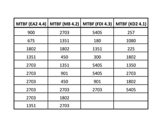
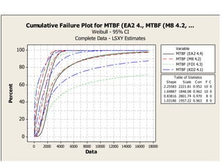
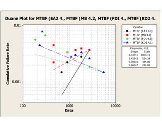
The document discusses methods to enhance RAM (reliability, availability, maintainability) of systems. It provides a regression equation that models availability percentage as a function of reliability and maintainability percentages, based on analysis of data from different machines. Various graphs and statistical analyses are also presented to compare mean time between failures (MTBF) of the machines and identify differences between them.

1. How to Enhance RAM
• By
Dr. Bikram Jit Singh
Professor
MMDU Mullana
Haryana

2. MTBF (EA2 4.4) MTBF (M8 4.2) MTBF (FDI 4.3) MTBF (KD2 4.1)
900 2703 5405 257
675 1351 180 1080
1802 1802 1351 225
1351 450 300 1802
2703 1351 5405 1350
2703 901 5405 2703
2703 450 901 1802
2703 2703 2703 5405
2703 1802
1351 2703

3. 10000100010010
90
50
10
1
Data
Percent
100000100001000100
99
90
50
10
1
DataPercent
10000100010010
90
50
10
1
Data
Percent
10000010000100010010
99
90
50
10
1
Data
Percent
MTBF (EA 2 4.4)
MTBF (M8 4.2)
MTBF (FDI 4.3)
MTBF (KD2 4.1)
V ariable
Weibull
0.952, 0.962, 0.970, 0.963
Lognormal
0.913, 0.942, 0.949, 0.957
Exponential
*, *, *, *
Loglogistic
0.908, 0.937, 0.944, 0.957
C orrelation C oefficient
Probability Plot for MTBF (EA2 4., MTBF (M8 4.2, MTBF (FDI 4., ...
LSXY Estimates-Complete Data
Weibull Lognormal
Exponential Loglogistic

4. 1000001000010001001010.1
99
90
80
70
60
50
40
30
20
10
5
3
2
1
Data
Percent
2.25583 2221.81 0.952 10 0
1.69887 1848.08 0.962 10 0
0.83816 2801.74 0.970 8 0
1.03186 1957.22 0.963 8 0
Shape Scale C orr F C
Table of Statistics
MTBF (EA2 4.4)
MTBF (M8 4.2)
MTBF (FDI 4.3)
MTBF (KD2 4.1)
Variable
Probability Plot for MTBF (EA2 4., MTBF (M8 4.2, MTBF (FDI 4., ...
Complete Data - LSXY Estimates
Weibull - 95% CI

5. 180001600014000120001000080006000400020000
100
80
60
40
20
0
Data
Percent
2.25583 2221.81 0.952 10 0
1.69887 1848.08 0.962 10 0
0.83816 2801.74 0.970 8 0
1.03186 1957.22 0.963 8 0
Shape Scale C orr F C
Table of Statistics
MTBF (EA2 4.4)
MTBF (M8 4.2)
MTBF (FDI 4.3)
MTBF (KD2 4.1)
Variable
Survival Plot for MTBF (EA2 4., MTBF (M8 4.2, MTBF (FDI 4., ...
Complete Data - LSXY Estimates
Weibull - 95% CI

6. 180001600014000120001000080006000400020000
100
80
60
40
20
0
Data
Percent
2.25583 2221.81 0.952 10 0
1.69887 1848.08 0.962 10 0
0.83816 2801.74 0.970 8 0
1.03186 1957.22 0.963 8 0
Shape Scale C orr F C
Table of Statistics
MTBF (EA2 4.4)
MTBF (M8 4.2)
MTBF (FDI 4.3)
MTBF (KD2 4.1)
Variable
Cumulative Failure Plot for MTBF (EA2 4., MTBF (M8 4.2, ...
Complete Data - LSXY Estimates
Weibull - 95% CI

7. 18000
16000
14000
12000
10000
8000
6000
4000
20000
0.007
0.006
0.005
0.004
0.003
0.002
0.001
0.000
Data
Rate
2.25583 2221.81 0.952 10 0
1.69887 1848.08 0.962 10 0
0.83816 2801.74 0.970 8 0
1.03186 1957.22 0.963 8 0
Shape Scale C orr F C
Table of Statistics
MTBF (EA2 4.4)
MTBF (M8 4.2)
MTBF (FDI 4.3)
MTBF (KD2 4.1)
Variable
Hazard Plot for MTBF (EA2 4., MTBF (M8 4.2, MTBF (FDI 4., MTBF (KD2 4.
Complete Data - LSXY Estimates
Weibull

8. MTBF (KD2 4.1)
MTBF (FDI 4.3)
MTBF (M8 4.2)
MTBF (EA2 4.4)
6000500040003000200010000
11 11 11 11
11 111 11 1
11 11 1 11 11 1
1 111111 11 1
Data
Event Plot for MTBF (EA2 4., MTBF (M8 4.2, MTBF (FDI 4., MTBF (KD2 4.

9. 6000500040003000200010000
20
15
10
5
0
Data
MCF
2.33741 1009.19
1.45343 554.34
0.78710 385.00
0.66047 232.00
Shape Scale
Parameter, MLE
MTBF (EA2 4.4)
MTBF (M8 4.2)
MTBF (FDI 4.3)
MTBF (KD2 4.1)
Variable
Mean Cumulative Function for MTBF (EA2 4., MTBF (M8 4.2, ...
95% CI

10. 100001000100
0.01
0.001
Data
CumulativeFailureRate
2.33741 1009.19
1.45343 554.34
0.78710 385.00
0.66047 232.00
Shape Scale
Parameter, MLE
MTBF (EA2 4.4)
MTBF (M8 4.2)
MTBF (FDI 4.3)
MTBF (KD2 4.1)
Variable
Duane Plot for MTBF (EA2 4., MTBF (M8 4.2, MTBF (FDI 4., MTBF (KD2 4.

11. 1.00.80.60.40.20.0
1.0
0.8
0.6
0.4
0.2
0.0
Scaled Failure Number
ScaledTotalTimeonTest
2.33741 1009.19
1.45343 554.34
0.78710 385.00
0.66047 232.00
Shape Scale
Parameter, MLE
MTBF (EA2 4.4)
MTBF (M8 4.2)
MTBF (FDI 4.3)
MTBF (KD2 4.1)
Variable
Total Time on Test Plot for MTBF (EA2 4., MTBF (M8 4.2, ...

12. Tm (hrs) for FDI 4.3 Tm (hrs) for EA2 4.4 Tm (hrs) for M8 4.2 Tm (hrs) for KD2 4.1
3.416 5 0.00037 5.25
17.833 9.833 0.00074 5.416
6.666 12.333 0.000555 35.333
51.416 8.416 0.001111 6.166
5.25 9 0.00074 26.5
5.25 3 0.000555 4
2.75 2.833 0.00074 6.25
6.583 1.166 0.00037 0.833
1 0.000555
2.5 0.00037

13. Differences among the means are significant (p < 0.05).
> 0.50.10.050
NoYes
P = 0.002
Tm (hrs) f_1
Tm (hrs) f_4
Tm (hrs) f_2
Tm (hrs) f_3
3020100
difference to determine if it has practical implications.
are the most likely to differ. Consider the size of the
least amount of overlap are red, and indicate the means that
Chart to identify means that differ. The intervals with the
means at the 0.05 level of significance. Use the Comparison
You can conclude that there are differences among the
1 Tm (hrs) f_3 4
2 Tm (hrs) f_2
3 Tm (hrs) f_4
4 Tm (hrs) f_1 1
# Sample Differs from
Which means differ?
One-Way ANOVA for Tm (hrs) f_1, Tm (hrs) f_2, Tm (hrs) f_3,...
Summary Report
Do the means differ?
Means Comparison Chart
The red intervals are the most likely to differ.
Comments

14. at most a 60% chance of detecting a difference of 4.0200.
least a 90% chance of detecting a difference of 31.419, and
Based on your samples and alpha level (0.05), you have at
100%
31.419
90%
4.0200
60%< 40%
4.0200 5.3 - 60.0
22.068 60.0 - 100.0
24.560 70.0 - 100.0
27.475 80.0 - 100.0
31.419 90.0 - 100.0
Difference Power
with your sample sizes?
What difference can you detect
Tm (hrs) f_1 8 12.395 16.451 (-1.3583, 26.149)
Tm (hrs) f_2 10 5.5081 4.0533 (2.6085, 8.4077)
Tm (hrs) f_3 10 0.00061 0.00023 (0.00044, 0.00078)
Tm (hrs) f_4 8 11.218 12.504 (0.76463, 21.672)
Sample Size
Sample
Mean Deviation
Standard
95% CI for Mean
Individual
Statistics
27.475, consider increasing the sample sizes.
Power is a function of the sample sizes and the standard deviations. To detect differences smaller than
One-Way ANOVA for Tm (hrs) f_1, Tm (hrs) f_2, Tm (hrs) f_3,...
Power Report
Power
What is the chance of detecting a difference?

15. Tm (hrs) for KD2 4.1Tm (hrs) for M8 4.2Tm (hrs) for EA2 4.4Tm (hrs) for FDI 4.3
50
40
30
20
10
0
Data
6.583
2.750
5.2505.250
51.416
6.666
17.833
3.416 2.500
1.0001.166
2.8333.000
9.000
8.416
12.333
9.833
5.000
0.0003700.0005550.0003700.0007400.0005550.0007400.0011110.0005550.0007400.000370
0.833
6.250
4.000
26.500
6.166
35.333
5.4165.250
Individual Value Plot

16. Tm (hrs) for KD2 4.1Tm (hrs) for M8 4.2Tm (hrs) for EA2 4.4Tm (hrs) for FDI 4.3
50
40
30
20
10
0
Data
5.9165
4
0.000555
5.791
12.3955
5.5081
0.0006106
11.2185
51.416
Boxplot for Given Machines

17. The regression equation is
Availability % = 93.2 + 0.056 Reliability % + 0.002 Maintainability %