REGULAR ARTICLEShoot hydraulic characteristics, plant wate.docx

REGULAR ARTICLE
Shoot hydraulic characteristics, plant water status
and stomatal response in olive trees under different
soil water conditions
J. M. Torres-Ruiz & A. Diaz-Espejo & A. Morales-Sillero &
M. J. Martín-Palomo & S. Mayr & B. Beikircher &
J. E. Fernández
Received: 8 March 2013 /Accepted: 13 May 2013 /Published
online: 4 June 2013
Abstract
Aims To evaluate the impact of the amount and distri-
bution of soil water on xylem anatomy and xylem
hydraulics of current-year shoots, plant water status
and stomatal conductance of mature ‘Manzanilla’ ol-
ive trees.
Methods Measurements of water potential, stomatal
conductance, hydraulic conductivity, vulnerability to
embolism, vessel diameter distribution and vessel den-
sity were made in trees under full irrigation with non-
limiting soil water conditions, localized irrigation, and
rain-fed conditions.
Results All trees showed lower stomatal conductance
values in the afternoon than in the morning. The irri-
gated trees showed water potential values around −1.4
and −1.6 MPa whereas the rain-fed trees reached lower
values. All trees showed similar specific hydraulic con-
ductivity (Ks) and loss of conductivity values during the

morning. In the afternoon, Ks of rain-fed trees tended to
be lower than of irrigated trees. No differences in vul-
nerability to embolism, vessel-diameter distribution and
vessel density were observed between treatments.
Conclusions A tight control of stomatal conductance
was observed in olive which allowed irrigated trees to
avoid critical water potential values and keep them in a
safe range to avoid embolism. The applied water treat-
ments did not influence the xylem anatomy and vul-
nerability to embolism of current-year shoots of ma-
ture olive trees.
Keywords Cavitation . Olive . Irrigation .
Vulnerability to drought-induced embolism . Water
stress . Xylem anatomy
Introduction
According to the cohesion theory (Dixon and Joly 1894;
Askenasy 1895) water ascends plants in a metastable
state. The driving force is generated by the negative
pressure at the evaporating surfaces of the leaf. The
tension is transmitted through a continuous water col-
umn from leaves to roots and lowers their water poten-
tial below the potential of the surrounding soil. This
causes water uptake from the soil and its upward move-
ment to the aerial part of the plant. The decrease in water
potential as the soil gets dry may cause cavitation of
Plant Soil (2013) 373:77–87
DOI 10.1007/s11104-013-1774-1
Responsible Editor: Rafael S. Oliveira.
J. M. Torres-Ruiz (*) : A. Diaz-Espejo : J. E. Fernández

Irrigation and Crop Ecophysiology Group, Instituto
de Recursos Naturales y Agrobiología de Sevilla
(IRNAS, CSIC), Avenida Reina Mercedes, n.º 10,
41012 Sevilla, Spain
e-mail: [email protected]
A. Morales-Sillero : M. J. Martín-Palomo
Departamento de Ciencias Agroforestales, ETSIA,
University of Sevilla, Carretera de Utrera, km 1,
41013 Seville, Spain
S. Mayr: B. Beikircher
Department of Botany, University of Innsbruck,
Sternwartestr. 15, 6020 Innsbruck, Austria
# European Union 2013
conduits and the resulting embolism to loss of hydraulic
conductivity (K) (Tyree and Zimmerman 2002). Stoma-
tal closure is one of the most effective mechanisms to
avoid critical water potential values (Choat et al. 2012).
Accordingly, also olive trees minimize water losses
under high water demand conditions by stomata regula-
tion (Fernández et al. 1997; Tognetti et al. 2009;
Boughalleb and Hajlaoui 2011). Stomatal closure is
known to be especially advantageous in environ-
ments with wide fluctuations both in evaporative
demand and soil moisture (Franks et al. 2007), as
those in which the olive tree is widely grown
(Fernández and Moreno 1999).
The relationships between stomatal conductance
(gs), leaf water potential (Ψl), K and environmental
variables are complex. Feedback mechanisms between
these variables (Chaves et al. 2003; Lovisolo et al.

2010) and differences between cultivars (Winkel and
Rambal 1990; Fernandez et al. 2008) have been
reported. In addition, irregular distribution of water
in the rootzone may trigger root-to-shoot signals in-
ducing stomatal closure (Dry and Loveys 1999; Dodd
2005). This is caused by some irrigation systems, as
localized irrigation, in which a fraction only of the
rootzone is wetted by irrigation. In olive, Fernández
et al. (2003) reported restricted transpiration in trees
under localized irrigation, but they could not unravel
whether the stomatal closure was induced by a chem-
ical signal involving abscisic acid (ABA) generated in
the roots remaining in the drying soil or by a hydraulic
signals, as e.g. the drop of hydraulic conductance,
caused by soil drying. Bacelar et al. (2007) analyzed
the effect of the soil water regime on gas exchange and
xylem hydraulic properties of olive cultivars. They
reported that water stress caused a marked decline of
gs and an increase in xylem vessel density in all
cultivars. Some of those cultivars also showed a re-
duction in vessel diameter. They worked, however,
with 1-year-old plants in pots and their experiments
did not include localized irrigation. Tognetti et al.
(2009) reported that the loss of hydraulic conductance
is an important signal for the stomatal control of tran-
spiration in olive trees under drying soil conditions. A
better understanding of how soil water regime and plant
water status influence stomata regulation and hydraulics
of olive cultivars is important for a efficient manage-
ment of water used in irrigated orchards. The interest in
this area of research is considerable given that 2.3 out of
the 10.5 Mha of olive surface are irrigated, mostly with
localized irrigation systems (International Olive Coun-
cil, www.internationaloliveoil.org; Pastor 2005).

We evaluated the effect of different soil water re-
gimes on xylem anatomy, xylem hydraulics and gas
exchange in current-year shoots of mature ‘Manzanil-
la’ olive trees. Measurements of xylem anatomical
parameters, Ψl, gs, specific hydraulic conductivity
(Ks) and percentage loss of conductivity (PLC) and
analysis of the vulnerability to embolism were made in
41-year-old ‘Manzanilla’ olive trees along a full irri-
gation season. The trees were under three different soil
water regimes: rain-fed conditions, localized irrigation
in which part of the rootzone remained in drying soil,
and full irrigation that kept the whole rootzone under
non-limiting soil water conditions. We hypothesized
that differences in soil water conditions imposed by
the mentioned water treatments limit plant hydraulics
and lead to stomatal regulations as well as to acclima-
tion in xylem anatomical traits in olive trees.
Materials and methods
Experimental site and water treatments
This study was carried out at ‘La Hampa’ experimental
farm, 15 km from Seville, southwest Spain (37º 17′ N, 6º
3′ W, 30 m a.s.l.). Climate in the area is Mediterranean
with a wet, mild season from October to April and a hot,
dry season from May to September. Trees in the orchard
were 41-year-old ‘Manzanilla de Sevilla’ (from now on
‘Manzanilla’) olive trees at 7 m×5 m spacing (286 trees
ha−1). The soil of the orchard is a sandy loam
(Xerochrept) of 1.6–2.0 m depth. The texture is quite
homogeneous, both vertically and horizontally (Moreno
et al. 1988), with mean values of 14.8 % clay, 7.0 % silt,
4.7 % fine sand and 73.5 % coarse sand. Laboratory
measurements showed a volumetric soil water content
(θv) of 0.33 and 0.09 m

3 m−3 for a soil matric potential of
−0.01 and −1.5 MPa respectively. Field measurements
showed θv=0.22 m
3 m−3 at field capacity conditions.
Experiments were made during the irrigation season
of 2009, from May 6, day of year (DOY) 126, to
October 2 (DOY 275). Three adjacent 0.2 ha plots were
used in the project, each under a different water treat-
ment: 1) a rain-fed treatment (R), in which rainfall was
the only source of water supply until a recovery irriga-
tion was applied from September 8 (DOY 251) to the
end of the season. This consisted on supplying daily
78 Plant Soil (2013) 373:77–87
three times more water than to the LI trees (described
below), in a circle of ca. 2 m radius around the trees; 2)
Localized irrigation (LI), in which trees were irrigated
daily throughout the irrigation season with enough wa-
ter to replace 100 % of the crop evapotranspiration
(ETc). The irrigation system consisted of a lateral pipe
per tree row with five 3 L h−1 drippers per tree, 1 m
apart. This system leaves part of the roots under soil
drying conditions during the irrigation season. The irri-
gation dose was calculated with the crop coefficient
approach (Allen et al. 1998), with coefficients adjusted
for the orchard conditions by Fernández et al. (2006);
and 3) Full irrigation (FI), in which trees were irrigated
with a 0.4 m×0.4 m grid of pipes with a 2 L hour−1
dripper in every node. The grid covered a surface of

8 m×6 m, with the tree in the middle, enough to keep
non-limiting soil water conditions in the whole rootzone
throughout the irrigation season. The FI trees were
irrigated every other day, to avoid hypoxia.
Soil water and weather measurements
Soil water profiles were measured every 7–10 days
during the experimental period. We used a PR2-Profile
probe (Delta-T Devices Ltd, Cambridge, UK) with three
access tubes per tree in three trees per treatment, at
0.50 m, 1.50 m and 2.25 m from the trunk to cover
possible heterogeneities in soil water distribution. In
each access tube θv values were measured at 0.1, 0.2,
0.3, 0.4, 0.6 and 1.0 m depth. These values were used to
calculate the relative extractable water (REW) according
to Granier (1987). Simultaneous measurements of root
distribution and soil water content in the orchard down
to 2.4 m depth made by Fernández et al. (1991) showed
that the explored top meter of soil was enough for a
reliable average value of θv in the rootzone of the
experimental trees.
Main weather variables were recorded every 30 min
with a weather station (Campbell Scientific Ltd., Leices-
tershire, UK) under standard conditions, located at ca.
50 m from the orchard. These data were used to calcu-
late the FAO56 Penman-Monteith potential evapotrans-
piration, ETo (Allen et al. 1998).
Leaf water potential and stomatal conductance
Values of Ψl at predawn, in the morning (9–10 GMT)
and in the afternoon (14–15 GMT) were measured on
June 23 (DOY 175), July 28 (DOY 209), August 25

(DOY 237) and October 1 (DOY 274). We sampled two
fully expanded leaves of the current year per tree in three
trees per treatment. Measurements were made with a
Scholander-type pressure chamber (Soilmoisture Equip-
ment Corp., Santa Barbara, California, USA), following
recommendations by Turner (1988) and Koide et al.
(1989). We measured gs at the same time as Ψl both in
the morning and in the afternoon. We used a LI-6400
portable photosynthesis system (Licor Inc., USA) and
sampled the same type and number of leaves as for Ψl.
Hydraulic conductivity and native embolism
Five branches per treatment of 1.2 m in length with at
least one 0.4 m long current-year shoot, respectively,
were cut under water (to avoid air entering into the
vessels), wrapped in plastic bags with wet paper towel
inside (to prevent transpiration) and transported to the
laboratory. To avoid any possible influence of the
sampling position on the results, all branches were
sampled from similarly-oriented parts of the canopy,
at ca. 1.5 m above ground. The sampling was made at
the same time, in the same trees and from the same
part of the canopy as the gs and Ψl measurements.
Once in the laboratory, we submerged one current-
year shoot of each branch in a container with perfusion
solution (see below). From each shoot we sampled one
ca. 30 mm long segment under water, removed its bark
and trimmed sample ends with a razor blade. All the
sampled segments were collected from the mid-part of
the shoots. The native K of each segment was then
determined with a XYL’EM® apparatus (Bronkhorst,
Montigny-les-Cormeilles, France) as:
K ¼ F
ΔP

L ð1Þ
where F mass flow rate of a solution through the
segment, ΔP is the applied pressure gradient driving
the flow and L is the sample length. We used a filtered
(0.22 μm) 50 mM KCl perfusion solution made with
distilled water, and applied a pressure gradient of 3 kPa
until a steady-state native K was attained. Previous
experiments in olive showed that this water head is
below the threshold at which embolized vessel opened
at both ends are flushed and artificially contribute to K
(data not shown). Flushing was obtained after initial K
measurements by perfusion at 150 kPa for 20 min. The
pressure was then lowered again down to 3 kPa to
Plant Soil (2013) 373:77–87 79
determine maximum K. Percent loss of conductivity
(PLC) (i.e. native embolism) was calculated as:
PLC ¼ 100 � 1−native K
.
maximum K
� �
ð2Þ
The Ks was calculated by dividing native K by the
mean cross-sectional area of the sample.
Vulnerability curves
On November 2 (DOY 306), twenty 1.5 m long branches

with 3–4 current-year shoots, respectively were sampled
under water from 3 to 5 representative trees of each
treatment, and transported to the laboratory as described
above. The branches were used to determine vulnerabil-
ity to drought-induced embolism by the bench-top dry-
ing technique (Tyree and Dixon 1986; Sperry and Tyree
1988). During dehydration, xylem water potential (Ψx)
was measured in intervals until the desired values down
to −10 MPa were reached. Branches then were stored for
1.5 h in a plastic bag with a wet paper towel inside to
allow the equilibrium between Ψl and Ψx. Measurements
of Ψx were made in two leaves per branch and after-
wards, one segment of ca. 30 mm length per current-year
shoot was sampled, following the procedure described
above for native K measurements and PLC determina-
tions. We generated one vulnerability curve per treatment
by plotting PLC versus Ψx. For fitting the vulnerability
curves obtained from each treatment we used a Weibull
function (Neufeld et al. 1992) with an additional inde-
pendent factor to consider the levels of embolism mea-
sured at Ψx≃0:
PLC ¼ 100−y0ð Þ− 100−y0ð Þe−
x
bð Þc þ y0 ð3Þ
being x the Ψx, b the Ψx for a PLC of 63 %, c a
dimensionless parameter controlling the shape of the
curve and y0 the PLC at Ψx=0 MPa. These points were
fitted to Eq. 3 using Excel’s solver function. The Ψx
IA
(
m

m
)
0
5
10
15
20
P
(
m
m
)
0
2
4
6
8
10
FI
LI

R
E
T
(
m
m
)
0
2
4
6
8 ETo
ETc
DOY 2009
120 140 160 180 200 220 240 260 280
R
E
W
0,0
0,5
1,0

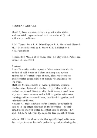
FI
LI
R
May June July August September October
a
b
c
Fig. 1 Time courses of
(a) reference (ETo) and crop
evapotranspiration (ETc),
b collected precipitation (P)
and irrigation amounts (IA)
supplied to trees of each
treatment, and (c) relative
extractable water (REW)
for each treatment. DOY day
of year. Arrows indicate
sampling dates for variables
shown in Figs. 2, 3 and 4
80 Plant Soil (2013) 373:77–87
values corresponding to 50 % loss of hydraulic conduc-
tivity (P50, MPa) due to embolism formation and its
95 % confidence intervals were calculated from each
vulnerability curve.
Anatomical measurements

On November 2 (DOY 306), current-year shoots of
similar characteristics than those used for K measure-
ments were collected from four different representa-
tive trees per treatment. One 10 mm segment was
sampled from each shoot, dehydrated in an acetone
series and embedded in SPURR resin. Sections were
cut with an ultramicrotome, stained with toluidine blue
(1 %) for 3 min, rinsed in water and photographed
with a digital camera attached to a light microscope
(Olympus BX61). Images from each section were
divided into four parts of similar area. Vessel density
(number of vessels in a given area) was determined in
two of these parts using Adobe Photoshop CS3 soft-
ware (Adobe Systems Incorporated, USA). The vessel
diameter was calculated for each vessel from its sur-
face area, previously determined with the mentioned
software, assuming a circularity of 1. The diameter
distribution per treatment was determined after classi-
fying the vessels into bin diameters (diameter size
classes of 2 μm width). The resulting values were
expressed as percentage of vessel number from total
in each class. Some 300 to 500 vessels were measured
per section.
Statistical analysis
Data sets were tested for normality with the Kolmogorov-
Smirnov test and homogeneity of variances was deter-
mined by Brown & Forsythe test. Differences in Ψl, gs, K,
PLC, vessel density and percentage of vessel in each bin
diameter between water treatments were evaluated by a
one-way analysis of variance (ANOVA). When the dif-
ferences were significant, a multiple comparison of
means (post hoc Tukey honest significant difference test)

was carried out. Statistical comparisons were considered
significant at p<0.05. P50 values calculated from the
vulnerability curves obtained for trees of each water
treatment were considered significantly different when
their 95 % confidence intervals did not overlap.
Repeated measures analyses of variance (ANOVA)
over time were carried out to test differences in Ψl, gs,
K and PLC between FI and LI trees during the season.
All analyses were performed by using STATISTICA
software (StatSoft, Inc., USA) and Sigmaplot (SPSS
Inc., USA).
Results
Weather conditions and soil moisture
Except for peak values of ETo recorded at the end of
May, the time course of the atmospheric demand dur-
ing the experimental period was as usual in the area,
with high values in the middle of the summer and
decreasing values from the end of August (Fig. 1a).
P
re
d
a
w
n
l
(M

P
a
)
-6
-5
-4
-3
-2
-1
0
FI
LI
R
M
o
rn
in
g
l
(M
P
a
)

-6
-5
-4
-3
-2
-1
160 180 200 220 240 260 280
A
ft
e
rn
o
o
n
l
(M
P
a
)
-6

-5
-4
-3
-2
-1
DOY 2009
June July August September
a
a
b
a
a
b
a
a
b
n.s.
a
a
b

a
a
b
a
a
b
a
b
c
a
a
b
a
a
b
a
a
b
n.s
a

b
c
Fig. 2 Time courses of leaf water potential (Ψl) measured at (a)
predawn, b at 9.00–10.00 GMT (morning Ψl), and (c) at 14.00–
15.00 GMT (afternoon Ψl). Data points are average of six
values; vertical bars represent ± the standard error. Different
letters indicate statistically significant difference (p<0.05) be-
tween treatments. n.s. no significant difference. The dashed line
indicates the beginning of the recovery irrigation applied to the
R trees. DOY day of year
Plant Soil (2013) 373:77–87 81
The irrigation amounts applied to the LI trees (Fig. 1b)
were enough to maintain REW values close to field
capacity throughout the irrigation season (Fig. 1c). In
the FI plot, REW values showed conditions close to
saturation. Total amounts of water supplied to LI and
FI trees were 3361.8 m3 ha−1 (88 % ETc) and
16121 m3 ha−1 (420 % ETc), respectively. The high
irrigation supplies in the FI treatment were justified by
the need of ensuring non-limiting soil water conditions
in the whole rootzone. REW values in the R plot de-
creased during the irrigation season, until the recovery
irrigation applied from DOY251 to DOY275, when
1482.3 m3 ha−1 of water were supplied. This, together
with the first rainfall events after the summer dry period
(Fig. 1b) increased REW values to ca. 0.9 (Fig. 1c).
Plant water status and stomatal conductance

Similar values of Ψl at predawn were recorded in the
LI and FI trees during the dry season (Fig. 2a). In
contrast, R trees showed decreasing Ψl values at
predawn throughout the summer, in agreement with
the gradual decrease in REW (Fig. 1c). In the LI and
FI trees, Ψl values were close to −1.5 MPa both in the
morning and the afternoon throughout the dry season
(Figs. 2b and c), indicating no increase in water stress
during the season. Although slightly, the Ψl was
M
o
rn
in
g
g
s
(m
o
l m
-2
s
-1
)
0,00
0,05

0,10
0,15
0,20
0,25
0,30
FI
LI
R
DOY 2009
160 180 200 220 240 260 280
A
ft
e
rn
o
o
n
g
s
(m
o

l m
-2
s
-1
)
0,00
0,05
0,10
0,15
0,20
0,25
a
b
c
a
ab
b
a
a

b
a
a
b
a
a
b
a
ab
b
a
a
b
a
a
b
June July August September
a
b

Fig. 3 Time courses of sto-
matal conductance (gs) mea-
sured at (a) ca. 9.00–10.00
GMT and (b) 14.00–15.00
GMT. Data points are aver-
age of six values; vertical
bars represent ± the standard
error. Different letters indi-
cate statistically significant
difference (p<0.05). The
dashed line indicates the be-
ginning of the recovery irri-
gation applied to the R trees.
DOY day of year
Table 1 Values of the vapour pressure deficit of the air (Da)
recorded in the morning (9–10 GMT) and in the afternoon (14–
15 GMT) of the days when main physiological variables were
measured
DOY Da (kPa)
Morning Afternoon
174 1.47 3.73
209 2.10 4.66
234 1.85 3.42
274 0.30 1.65
82 Plant Soil (2013) 373:77–87

consistently lower in LI trees than in the FI trees during
the whole season (Table 3) but not on a day-by-day basis
(Fig. 2). In the R trees, Ψl values during the dry period
were significantly lower than in LI and FI trees. Simi-
larly to predawn, Ψl decreased in the R trees both in the
morning and in the afternoon throughout the season as
the soil water was depleted. The most negative values
were recorded at the end of August (morning Ψl=−4.2±
0.4 MPa; afternoon Ψl=−4.8±0.4 MPa), when lowest
REW were recorded (Fig. 1c). The water supplied by the
recovery irrigation and the rainfall events in autumn
(Fig. 1b) caused Ψl of R trees to raise to values similar
to LI and FI trees (Fig. 2).
In LI and FI trees, gs values in the morning were
over 0.2 mol m−2 s−1 during the entire dry season (i.e.
until the first rainfall events), while R trees showed
much lower gs values (Fig. 3a). In all trees, gs in the
afternoon was lower than in the morning during the
drought season but similar at the end of the study
period (Fig. 3). Both in the morning and in the after-
noon, the LI trees used to show lower gs values than
the FI trees although differences were not always
significant day by day. But, when the entire season is
considered, the gs was consistently lower in LI than in
FI (Table 3). Marked differences in Da between morn-
ing and afternoon were recorded during the whole
season (Table 1).
Hydraulic and anatomical characteristics
No pronounced differences or trends were observed
between treatments in Ks or PLC of morning samples
(Fig. 4a, b). In the afternoon, Ks in the R trees tended to
be lower than in the irrigated trees with significant

differences at DOY 209. In the FI and LI trees, no
significant differences or trends in Ks or PLC were
found, either day by day or during the season (Fig. 4;
Table 3). Corresponding to the course in Ks, PLC of R
trees peaked at DOY 209 (ca. 60 %), while PLC values
were similar on all other sampling days (Fig. 4c, d).
Trees from all treatments showed a similar vulnera-
bility to embolism (Fig. 5a) and no difference between
P50 (Table 2). Figure 5a shows that native PLC at Ψx
close to 0 MPa was 15–30 % in all treatments. Accord-
ingly, anatomical analysis revealed similar vessel diam-
eter distributions in all treatments (Fig. 6). Vessel den-
sity tended to be highest in R trees, followed by LI and
FI trees, but differences were not significant (Table 2).
DOY 2009
160 180 200 220 240 260
P
L
C
0
20
40
60
80
160 180 200 220 240 260 280

Afternoon
n.s.
n.s.
n.s.n.s.
n.s.
n.s.
n.s. n.s.
n.s.
n.s. n.s.
n.s.
a
b d
June July August September June July August September
n.s.
n.s.
n.s.
a
a
bc
Morning

K
s
(k
g
m
-1
s
-1
M
P
a
-1
)
0.0
0.1
0.2
0.3
0.4
0.5
0.6
0.7

FI
LI
R
Fig. 4 Average values of specific hydraulic conductivity (Ks)
and percentage loss of hydraulic conductivity (PLC) at 9.00–
10.00 GMT (i.e. morning) (a, b respectively) and at 14.00–
15.00 GMT (c, d respectively) (i.e. afternoon). Data points are
average of three to five values; vertical bars represent±the
standard error. Different letters indicate statistically significant
difference (p<0.05); n.s. no significant difference. The dashed
lines show the beginning of the recovery irrigation applied to
the
R trees. DOY day of year
Plant Soil (2013) 373:77–87 83
Discussion
Stomatal control of transpiration and embolism
formation
Results of the present study suggest a tight control of Ψl
in olive (Fig. 3a, b). Despite of the two-fold increase in
Da between morning and afternoon (Table 1), Ψl was
maintained fairly constant and around 1.4–1.6 MPa,
which allowed FI and LI trees to avoid critical Ψl values.
Critical thresholds in olive have been reported to be
around −1.5 MPa (Sofo et al. 2008). Differences in gs
between morning and afternoon were proportional to
those observed in Da (Fig. 4), assuring a good balance
between the increase in water demand and supply. This

behaviour is typical for olive, a species well adapted to
drought, with stomatal closure from early in the morning
as an efficient strategy to reduce water losses and thus
decreases in water potential (Fernández et al. 1997;
Cuevas et al 2010). Despite restrictive stomatal closure
recorded also in the R trees, these trees reached Ψl
values more than two-fold lower than irrigated
trees (Figs. 2 and 3).
Interestingly, similar PLC values (Fig. 4) were ob-
served in all treatments although only R trees were
exposed to low Ψl during the study. Since vulnerability
curves also reflected some native PLC, a recomputed
vulnerability curve based on data of all treatments was
constructed (Fig. 5b). This curve enabled to compute the
air entry pressure (Pe), indicating the threshold xylem
0
20
40
60
80
100
R
LI
FI
Pe
x (MPa)

-10 -9 -8 -7 -6 -5 -4 -3 -2 -1 0
P
L
C
0
20
40
60
80
Recomputed data
Recomputed vulnerability curve
Pe
b
a
Fig. 5 a Xylem vulnerability to embolism curves of current-
year shoots of FI (○), LI (white triangle) and R (white square)
trees, represented as the percentage loss of conductivity (PLC),
as a function of decreasing xylem water potential (Ψx). Data
points are the average of five to seven samples; vertical bars
represent ± the standard error. The dashed grey line indicates
50 % loss of hydraulic conductivity; b All data represented in
Fig. 5a were recomputed considering PLC=0 at Ψx=0, and the
resulting vulnerability curve fitted and plotted. The black
dashed line represents the tangent through the midpoint of the
vulnerability curve and its x-intercept represents the air entry

pressure (Pe) following Meinzer et al. (2009)
Table 2 Values both of the xylem tension inducing 50 % loss of
hydraulic conductivity (P50) and their 95 % confidence interval
(95 % CI). Also shown are the mean vessel densities (n=4)
found
in current-year shoots from trees of each treatment. P50 values
which 95 % CI do not overlap are considered significantly
differ-
ent. No significant differences were found on vessel density be-
tween treatments (p<0.05); SE = standard error
Treatment P50 (MPa) Vessel density
(vessels mm−2)
R −4.35 (−3.67;−4.97) 618±63 SE
LI −4.02 (−3.50;−4.52) 555±69 SE
FI −4.26 (−3.59;−4.91) 499±75 SE
Diameter classes ( m)
0 2 4 6 8 10 12 14 16 18 20 22 24 26 28 30 32 34 36
D
is
tr
ib
u
tio
n
(
%
)

0
2
4
6
8
10
12
14
16
18
20
FI
LI
R
Fig. 6 Xylem vessel diameter distribution measured in four
cross-sections per treatment from current-year shoots. From
300 to 500 vessels were measured per section. Vertical bars
represent ± the standard error. No significant differences were
found between treatments
84 Plant Soil (2013) 373:77–87

pressure at which loss of conductivity begins to increase
rapidly (Meinzer et al. 2009). In our case, Pe was around
−1.3 MPa, demonstrating that water potentials observed
in irrigated trees (i.e. FI and LI trees) were too high for
any relevant induction of embolism. We thus conclude
that their native embolisms were formed prior to our first
measurements, maybe in an early stage of xylogenesis.
During the study period, irrigated trees were obviously
able to keep their water potential in a safe range and to
avoid further embolism. It is well known that under non-
extreme conditions, gs is regulated to keep Ψl within a
safety margin avoiding the development of embolism
(Brodribb and Holbrook 2003; Cochard et al. 2002;
Meinzer et al. 2009; Choat et al. 2012). In contrast, R
trees were not able to balance water deficits: observed
minimum Ψl of ca. −4.8 MPa and maximum PLC of ca.
60 % (Figs. 2 and 3) correspond relatively well with the
vulnerability curve. The full recovery of Ψl and gs in the
R trees observed on DOY 274, after the water supplies
of September (Fig. 1b), agrees with the well known
capacity of the olive tree to recover quickly from water
stress after the summer dry period (Lavee and Wodner
1991; Moriana et al. 2007).
Heterogeneity in soil water distribution within the
rootzone of the LI trees can promote changes in the
hydraulic conductance of the soil–leaf pathway, which
may indirectly drive changes in gs and transpiration
(Sperry et al. 2002). This, therefore, would explain the
fact that the gs values recorded in trees with localized
irrigation systems (i.e. LI trees) tended to be lower than
in FI trees, which had access to water homogenously
distributed in the soil (Fig. 3; Table 3). Indeed, an
additional chemical root-to-shoot signalling mechanism
triggered in the LI trees by roots remaining under soil

drying conditions could also have influenced the sto-
matal behaviour (Dodd et al. 2008), although this
mechanism is still to be proven in olive. From a
similar study carried out on the same trees and under
the same treatments, Morales-Sillero et al. (2013)
recently reported that the reductions in gs observed
in LI trees also reduced the net photosynthesis rate
with regard the FI trees. They also reported that
localized irrigation improved oil quality but reduced
fruit yield as compared to an irrigation system able to
wet the whole rootzone. Although they did not eval-
uate water productivity in the orchard, they suggested
that it would be higher in orchards with localized
irrigation than in those with irrigation systems that
wet the whole rootzone.
Acclimation in xylem anatomy and function
The applied water treatments did not influence the
vulnerability to embolism (Fig. 5a, Table 2), although
a significant fraction of the new wood in shoots was
formed under the influence of the water treatments.
Intraespecific differences in xylem resistance induced
by soil moisture conditions have been reported for
some species (Choat et al. 2007; Beikircher and Mayr
2009; Fichot et al. 2010), while other studies found no
effects (Maherali et al. 2002; Cornwell et al. 2007).
Lacking differences in hydraulic safety in studied ol-
ive trees corresponded well with similarity in vessel-
diameter distribution and vessel density across water
treatments. Only the number of vessels per mm −2
tended to increase in trees with lower irrigation doses
(Table 2). Contrasting results on the effect of the water
regime on the xylem characteristics in olive have been

previously reported for different olives varieties
(Bacelar et al. 2007; Lopez-Bernal et al. 2010). These
discrepancies could be due, apart from differences
between cultivars, to the different age of the studied
material, since histological characteristics may differ
between young and adult olive trees (Lopez-Bernal et
al. 2010). In each case, our results, reject our hypoth-
esis about the influence of soil water conditions on the
xylem anatomy and vulnerability to embolism of
current-year shoots.
Table 3 Significances (p) of the differences in leaf water po-
tential (Ψl), stomatal conductance (gs), specific hydraulic con-
ductivity (Ks) and percentage loss of hydraulic conductivity
(PLC) during the season between full irrigated (FI) and
localized
irrigated (LI) trees calculated by using repeated measures
(ANOVA) over time tests
Ψl gs Ks PLC
Predawn Morning Afternoon Morning Afternoon Morning
Afternoon Morning Afternoon
p 0.025* 0.006* 0.019* 0.003* 0.000* 0.741 0.128 0.445 0.053
*Differences were considered significant when p<0.05
Plant Soil (2013) 373:77–87 85
Conclusions
Our results showed a tight control of gs in olive which

allowed irrigated trees to avoid critical Ψl values and
keep them in a safe range to avoid embolism. Marked
stomatal closure was also observed in the R trees, but
this did not impede Ψl values being lower in those
trees than in the FI and LI trees. Values of Ks tended to
be lower in the R than in the irrigated trees. All
treatments, however, showed similar PLC values.
The applied water treatments did not affect the vulner-
ability to embolism, vessel-diameter distribution and
vessel density of current-year shoots of mature ‘Man-
zanilla’ olive trees.
Acknowledgments This project was funding both by the
Spanish Ministry of Science and Innovation (research project
AGL2006-04666/AGR) and the Austrian Science Fund (FWF)
(project No. P20852-B16). We thank Antonio Montero for
helping us in a great number of measurements. J.M. Torres-
Ruiz held a doctoral fellowship from the Spanish Ministry of
Science and Innovation (BES-2007-17149, MCINN).
References
Allen R, Pereira LS, Raes D, Smith M (1998) Crop evapotrans-
piration. Guidelines for computing crop water require-
ments. Irrigation and Drainage Paper, No. 56. FAO, Rome
Askenasy E (1895) Über das Saftsteigen. Verhandl Naturhist
Med Ver Heidelberg, NF 5:325–345
Bacelar EA, Moutinho-Pereira JM, Goncalves BC, Ferreira HF,
Correia CA (2007) Changes in growth, gas exchange,
xylem hydraulic properties and water use efficiency of
three olive cultivars under contrasting water availability
regimes. Environ Exp Bot 60:183–192
Beikircher B, Mayr S (2009) Intraspecific differences in

drought
tolerance and acclimation in hydraulics of Ligustrum
vulgare and Viburnum lantana. Tree Physiol 29:765–775
Boughalleb F, Hajlaoui H (2011) Physiological and anatomical
changes induced by drought in two olive cultivars (cv
Zalmati and Chemlali). Acta Physiol Plant 33:53–65
Brodribb TJ, Holbrook NM (2003) Stomatal closure during leaf
dehydration, correlation with other leaf physiological traits.
Plant Physiol 132:2166–2173
Chaves MM, Maroco JP, Pereira JS (2003) Understanding plant
responses to drought—from genes to the whole plant.
Funct Plant Biol 30:239–264
Choat B, Sack L, Holbrook NM (2007) Diversity of hydraulic
traits in nine Cordia species growing in tropical forests
with contrasting precipitation. New Phytol 175:686–698
Choat B, Jansen S, Brodribb TJ, Cochard H, Delzon S et al
(2012) Global convergence in the vulnerability of forests to
drought. Nature 491:752–755
Cochard H, Coll L, Le Roux X, Ameglio T (2002) Unraveling
the effects of plant hydraulics on stomatal closure during
water stress in walnut. Plant Physiol 128:282–290
Cornwell WK, Bhaskar R, Sack L, Cordell S, Lunch CK (2007)
Adjustment of structure and function of Hawaiian
Metrosideros polymorpha at high vs. low precipitation.
Funct Ecol 21:1063–1071
Cuevas MV, Torres-Ruiz JM, Álvarez R, Jiménez MD, Cuerva
J, Fernández JE (2010) Assessment of trunk diameter var-
iation derived indices as water stress indicators in mature

olive trees. Agric Water Manage 97:293–1302
Dixon HH, Joly J (1894) On the ascent of sap. Ann Bot London
8:468–470
Dodd IC (2005) Root-to-shoot signalling: Assessing the roles of
‘up’ in the up and down world of long-distance signalling
in planta. Plant Soil 274:251–270
Dodd I, Egea G, Davies W (2008) Abscisic acid signalling when
soil moisture is heterogeneous: decreased photoperiod sap
flow from drying roots limits abscisic acid export to the
shoots. Plant Cell Environ 31:1263–1274
Dry PR, Loveys BR (1999) Grapevine shoot growth and sto-
matal conductance are reduced when part of the root sys-
tem is dried. Vitis 38:151–156
Fernández JE, Moreno F (1999) Water use by the olive tree. J
Crop Prod 2:101–162
Fernández JE, Moreno F, Cabrera F, Arrúe JL, Martín-Aranda J
(1991) Drip irrigation, soil characteristics and the root
distribution and root activity of olive trees. Plant Soil
133:239–251
Fernández JE, Moreno F, Girón IF, Blázquez OM (1997)
Stomatal control of water use in olive tree leaves. Plant
Soil 190:179–192
Fernández JE, Palomo MJ, Diaz-Espejo A, Giron IF (2003)
Influence of partial soil wetting on water relation parame-
ters of the olive tree. Agronomie 23:545–552
Fernández JE, Diaz-Espejo A, Infante JM, Durán P, Palomo
MJ, Chamorro V, Girón IF, Villagarcía L (2006) Water

relations and gas exchange in olive trees under regu-
lated deficit irrigation and partial rootzone drying.
Plant Soil 284:273–291
Fernandez JE, Diaz-Espejo A, D’Andria R, Sebastiani L,
Tognetti R (2008) Potential and limitations of improving
olive orchard design and management through modelling.
Plant Biosyst 142:130–137
Fichot R, Barigah TS, Chamaillard S, Le Thiec D, Laurans F,
Cochard H, Brignolas F (2010) Common trade-offs be-
tween xylem resistance to cavitation and other physiolog-
ical traits do not hold among unrelated Populus deltoids x
Populus nigra hybrids. Plant Cell Environ 33:1553–1568
Franks PJ, Drake PL, Froend RH (2007) Anisohydric but
isohydrodynamic: seasonally constant plant water potential
gradient explained by a stomatal control mechanism incor-
porating variable plant hydraulic conductance. Plant Cell
Environ 30:19–30
Granier A (1987) Evaluation of transpiration in a Douglas-fir
stand by means of sap flow measurements. Tree Physiol
3:309–320
Koide RT, Robichaux RH, Morse SR, Smith CM (1989) Plant
water status, hydraulic resistance and capacitance. In: Pearcy
RW, Ehleringer J, Mooney HA, Rundel PW (eds) Plant phys-
iological ecology. Chapman & Hall, London, pp 161–179
86 Plant Soil (2013) 373:77–87
Lavee S, Wodner M (1991) Factors affecting the nature of oil
accumulation in fruit of olive (Olea europaea L) cultivars.

J Hortic Sci 66:583–591
Lopez-Bernal A, Alcantara E, Testi L, Villalobos FJ (2010)
Spatial
sap flow and xylem anatomical characteristics in olive trees
under different irrigation regimes. Tree Physiol 30:1536–1544
Lovisolo C, Perrone I, Carra A, Ferrandino A, Flexas J,
Medrano H, Schubert A (2010) Drought-induced changes
in development and function of grapevine (Vitis spp.) or-
gans and in their hydraulic and non-hydraulic interactions
at the whole-plant level: a physiological and molecular
update. Funct Plant Biol 37:98–116
Maherali H, Williams BL, Paige KN, Delucia EH (2002)
Hydraulic differentiation of Ponderosa pine populations
along a climate gradient is not associated with ecotypic
divergence. Funct Ecol 16:510–521
Meinzer FC, Johnson DM, Lachenbruch B, McCulloh KA,
Woodruff DR (2009) Xylem hydraulic safety margins in
woody plants: coordination of stomatal control of xylem
tension with hydraulic capacitance. Funct Ecol 23:922–930
Morales-Sillero A, García JM, Torres-Ruiz JM, Montero A,
Sánchez-Ortiz A, Fernández JE (2013) Is the productive
performance of olive trees under localized irrigation affect-
ed by leaving some roots in drying soil? Agric Water
Manage 123:79–92
Moreno F, Vachaud G, Martín-Aranda J, Vauclin M,
Fernández JE (1988) Balance hídrico de un olivar
con riego gota a gota. Resultados de cuatro años de
experiencias. Agronomie 8:521–537
Moriana A, Perez-Lopez D, Gomez-Rico A, Salvador MDD,

Olmedilla N, Ribas F, Fregapane G (2007) Irrigation
scheduling for traditional, low-density olive orchards:
water relations and influence on oil characteristics. Agric
Water Manage 87:171–179
Neufeld HS, Grantz DA, Meinzer FC, Goldstein G, Crisota GM,
Crisosto C (1992) Genotypic variability in vulnerability of
leaf xylem to cavitation in water-stressed and well-irrigated
sugarcane. Plant Physiol 100:1020–1028
Pastor M (2005) Cultivo del olivo con riego localizado. Junta de
Andalucia, Consejería de agricultura y pesca & Mundi-
Prensa.
Sofo A, Manfreda S, Fiorentino M, Dichio B, Xiloyannis C
(2008) The olive tree: a paradigm for drought tolerance in
Mediterranean climates. Hydrol Earth Syst Sci 12:293–301
Sperry JS, Tyree MT (1988) Mechanism of water stress-induced
xylem embolism. Plant Physiol 88:581–587
Sperry JS, Hacke UG, Oren R, Comstock JP (2002) Water
deficits and hydraulic limits to leaf water supply. Plant
Cell Environ 35:251–263
Tognetti R, Giovannelli A, Lavini A, Morelli G, Fragnito F,
d’Andria R (2009) Assessing environmental controls over
conductances through the soil-plant-atmosphere continuum
in an experimental olive tree plantation of southern Italy.
Agric Forest Meteorol 149:1229–1243
Turner NC (1988) Measurement of plant water status by the
pressure chamber technique. Irrigation Sci 9:289–308
Tyree MT, Dixon MA (1986) Water stress induced cavitation

and embolism in some woody plants. Physiol Plantarum
66:397–405
Tyree MT, Zimmerman MH (2002) Xylem structure and the
ascent of sap. Springer, New York
Winkel T, Rambal S (1990) Stomatal conductance of some
grapevines growing in the field under a Mediterranean
environment. Agric For Meteorol 51:107–121
Plant Soil (2013) 373:77–87 87
Copyright of Plant & Soil is the property of Springer Science &
Business Media B.V. and its
content may not be copied or emailed to multiple sites or posted
to a listserv without the copyright
holder's express written permission. However, users may print,
download, or email articles for
individual use.
Watch the two videos below
https://www.youtube.com/watch?v=09JTtVxztv4
https://www.youtube.com/watch?v=D7Q9i_wvd8U
216K views5 years ago

"Jamaica is embracing a controversial Super Bowl commercial
that depicts a white
office worker from the U.S. Midwest feigning ...
C
NEXT: BE SURE TO REVIEW THE SLIDES BELOW (msword
from ppt) FOR
DETAILED GUIDELINES ON THIS VERY EXCITING AND
REWARDING PROJECT.
● Approximately 3-4 pages, APA “modified” style format as we
have
reviewed in W1.
● 3 to 5 references expected earned
Project Overview
Header: An Intercultural Communication Analysis of “Get
Happy” VW
Commercials
Project Volkswagen Get Happy Super Bowl 2013 Full
Commercial!
● Project Overview: Do an analysis and critique of the
commercial (on
youtube.com) from the standpoint of the American culture and
do an
analysis and critique from a Jamaican cultural view.
● Your analysis and paper of this intercultural communication
case study
should focus on the following guidelines or parameters:

STEP ONE: Take an in-depth look (view it several times) at the
commercial itself.
Some questions to get you started are shown below
● What was its overall purpose of the VW commercial, in your
judgment?
● From your perspective, what was the commercial seeking to
accomplish?
● What was its creative intent as developed by the creative team
at the
agency?
https://www.youtube.com/watch?v=D7Q9i_wvd8U
STEP TWO: Next, examine and study the “Be (or Get) Happy”
Commercial from
an American cultural view
● What in your estimation, would be the general American view
of the
commercial?
● Is the ad racist in orientation in your judgment?
● Yes? Or No?
● Why? Or Why not?
● How would different American sub-cultures view the ad?
Select 1 or 2
for your commentary and analysis here.

STEP THREE: What is the critic's (American) view of the VW
Be Happy
commercial?
● What is the overall opinion of the American critics?
● What is the view of these critics? (such as Barbara Lippert)
● Were the critics predominantly positive or negative in their
view?
● If their view is either negative or positive, then why do you
think they
took the view they did?
STEP FOUR: What is the International view of the commercial
● How do you think the International community in general
viewed the
commercial(s)?
● Specifically, what view of the commercial did the Jamaican
government
take?
● Would the Jamaican view represent that of the greater
Caribbean island
nations?
● What did the Jamaican government publicly say vis a vis the
ad?
● How did the Jamaican government view the TV commercial,
in your
estimation?
● Interestingly, for this intercultural communication case study
were the

views of the Jamaican “people” and the government the same or
different?
STEP FIVE: What was the agency view of the commercial, in
your judgement?
● What do you think was the view of the agency (Deutsch LA)
as it
designed and produced the TV commercial?
● Did the agency perform “due diligence” (research) in
designing,
preparing, and producing the commercial?
● Did they do their homework?
● Did the agency produce an engaging commercial in your
estimation?
● What was the cost of a 30-second and 60-second commercial
for 2013
Super Bowl air time?
● Do you think that the client, VW, got its money's worth with
Be Happy?
STEP SIX: What did you learn about Intercultural
Communication from this
project?
● Specifically, what did you learn about different views of
intercultural

communication?
● What did you learn about your own understanding of how
cultures react
differently (and often unexpectedly) with regards to
intercultural
communication?
● Is there anything that you might recommend to do differently
in the role
of an intercultural communication consultant?
DELIVERABLES
● Approximately 3-4 pages, APA “modified” style format as
reviewed in
W1.
● 3 to 5 references expected
● Be prepared to review and share in an online class weekly
discussion &
dialog (Discussion Question) DQ
1400 Hydrological Sciences Journal – Journal des Sciences
Hydrologiques, 58 (7) 2013
http://dx.doi.org/10.1080/02626667.2013.829576
Impact of irrigation implementation on hydrology and water
quality in a
small agricultural basin in Spain

D. Merchán1 , J. Causapé1 and R. Abrahão2
1Geological Survey of Spain – IGME, C/ Manuel Lasala no. 44,
9◦B, Zaragoza, 50006, Spain
[email protected]
2Federal University of Paraíba – UFPB, Cidade Universitária,
João Pessoa, Paraíba, 58051-900, Brazil
Received 2 August 2012; accepted 10 January 2013; open for
discussion until 1 April 2014
Editor Z.W. Kundzewicz
Citation Merchán, D., Causapé, J., and Abrahão, R., 2013.
quality in a
small agricultural basin in Spain. Hydrological Sciences
Journal, 58 (7), 1400–1413.
Abstract Irrigation practice has increased considerably recently
and will continue to increase to feed a growing
population and provide better life standards worldwide.
Numerous studies deal with the hydrological impacts of
irrigation, but little is known about the temporal evolution of
the affected variables. This work assesses the effects
on a gully after irrigation was implemented in its hydrological
basin (7.38 km2). Flow, electrical conductivity,
nitrate concentration and exported loads of salts and nitrates
were recorded in Lerma gully (Zaragoza, Spain) for
eight hydrological years (2004–2011), covering the periods
before, during and after implementation of irrigation.
Non-parametric statistical analysis was applied to understand
relationships and trends. The results showed the cor-
relation of irrigation with flow and the load of salts and nitrates
exported, although no significant relationship with
precipitation was detected. The implementation of irrigation

introduced annual trends in flow (3.2 L s-1, +23%),
salinity (–0.38 mS cm-1, –9%), and nitrate concentration (5.4
mg L-1, +8%) in the gully. In addition, the annual
loads of contaminants exported increased (salts and nitrates,
27.3 Mg km-2 year-1, +19%, and 263 kg NO3--N
km-2 year-1, +27%, respectively). The trends presented a strong
seasonal pattern, with higher and more significant
trends for the irrigation season. The changes observed were
different from those of larger irrigation districts or
regional basins, due to the differences in land use and irrigation
management. It is important to understand these
changes in order to achieve an adequate management of the
environment and water resources.
Key words irrigation; trend; salinity; nitrate; contaminant loads;
land use
Impact de la mise en œuvre de l’irrigation sur l’hydrologie et la
qualité de l’eau dans un petit
bassin versant agricole en Espagne
Résumé Récemment, l’utilisation de l’irrigation a
considérablement augmenté, et elle va continuer à augmenter
pour nourrir une population croissante et fournir un meilleur
niveau de de vie à travers le monde. De nombreuses
études traitent des impacts hydrologiques de l’irrigation, mais
on connait peu de choses sur l’évolution temporelle
des variables affectées. Ce travail évalue les effets sur une
ravine, après que l’irrigation ait été mise en œuvre sur
son bassin hydrologique (7,38 km2). A cette fin, le débit, la
conductivité électrique, la concentration en nitrates
et les charges exportées de sels et de nitrates ont été
enregistrées sur la ravine de Lerma (Saragosse, Espagne)
pendant huit années hydrologiques (2004–2011), allant de la
période antérieures à la période postérieure à la
mise en œuvre de l’irrigation. Nous avons réalisé une analyse
statistique non paramétrique pour comprendre les

relations et les tendances. Les résultats ont montré une
corrélation entre l’irrigation d’une part, et le débit et les
charges exportées de sels et de nitrates d’autre part, mais
aucune relation significative avec les précipitations n’a
été détectée. La mise en œuvre de l’irrigation a provoqué une
évolution du débit (3,2 L s-1, +23%), de la salinité
(–0,38 mS cm-1, –9%), et de la concentration en nitrates (5,4
mg L-1, +8%) dans la ravine. En outre, la charge
annuelle de polluants exportée a augmenté (27,3 Mg km-2 an-1,
+19%, pour les sels, et 263 kg NO3-N km-2 an-1,
+27%, pour les nitrates). Les tendances présentent une forte
saisonnalité, et sont plus fortes et significatives pour
la saison d’irrigation. Les changements observés sont différents
de ceux de districts d’irrigation plus étendus ou
de bassins régionaux, cela étant dû aux différences dans
l’utilisation des terres et dans la gestion de l’irrigation. Il
est important de comprendre ces changements afin de parvenir à
une gestion adéquate de l’environnement et des
ressources en eau.
Mots clefs irrigation; tendance; salinité; nitrates; charges de
contaminants; utilisation des terres
© 2013 IAHS Press
quality in a small agricultural basin in Spain 1401
1 INTRODUCTION
There are many advantages to irrigated agriculture,
such as increased production, reliable harvests and
regional economic security (Duncan et al. 2008).
As a consequence, a global increase in irrigated areas

has been observed, especially in developing coun-
tries where, between 1962 and 1998, irrigated area
doubled (Food and Agriculture Organization (FAO
2003a). In Spain, the increase is moderate but signif-
icant, with 7% more irrigated area between 1990 and
2009 according to the Spanish environment min-
istry (Ministerio de Medio Ambiente y Medio Rural
y Marino; MMARM).
However, irrigation imposes sever pressure on
the environment, as it accounts for the consump-
tion of 70% of global water resources (FAO 2003b).
Water abstraction for irrigation purposes changes
hydrological conditions in dam-regulated rivers (Graf
2006), or overexploited aquifers (Custodio 2002).
These pressures impact on water resources not only
in a quantitative way, but also qualitatively (Kurunc
et al. 2005).
The impacts are not only found at the irrigation
water withdrawal location, as irrigation return flows
can cause hydrological changes in the receiving water
bodies. For this reason, organizations such as the US
Environmental Protection Agency see irrigated agri-
culture as the main source of water pollution (US
EPA 1992), particularly due to the leaching of salts
(Duncan et al. 2008) and nitrate (Arauzo et al. 2011,
Sánchez-Pérez et al. 2003), among other pollutants
(pesticides, phosphates, etc.).
Several studies exist on the hydrological changes
caused by irrigated agriculture. However, these stud-
ies were carried out either at such a large scale that
the influence of irrigation was masked by other factors
(water abstraction, industrial uses, etc.; CHE (2006),
or in areas where irrigation had already been imple-

mented (e.g. García-Garizábal and Causapé 2010, Qin
et al. 2011) without considering the dynamics of
irrigation implementation.
The impacts of irrigation are major issues in the
development of sustainable basin management strate-
gies. Irrigation affects land use and, therefore, causes
hydrological changes in the basin. The responses of
the basin to these changes need to be understood
(Zhang et al. 2011). Despite such an interest, to the
best of our knowledge, the study area of this work
is the first in which alteration induced by the trans-
formation from rainfed to irrigated agriculture has
been assessed, and this was achieved through the
monitoring of the hydrological basin during the tran-
sition. The research team has studied changes in this
study area for approximately ten years and several
papers have been published (Abrahão et al. 2011a,
2011b, 2011c, Peréz et al. 2011). A non-parametric
approach is used herein to deal with issues not treated
in previous research, such as trends in flow, water
quality parameters and exported loads of both salts
and nitrates, imposed by irrigation.
Within this framework, the aim of this work is
to analyse the effects of a newly-implemented irri-
gated area on the hydrology of a gully, evaluating
relationships between variables, and trends in flow,
water quality, and contaminant loads. This objec-
tive is consistent with the recommendations of local
water authorities (CHE 2006) that suggest the need
for increasing knowledge of water bodies with qual-
ity problems, in order to create management strategies
that will allow to control the quantity and quality of
water resources at the basin scale.

2 STUDY AREA AND BACKGROUND
The study area is Lerma gully and its hydrological
basin (7.38 km2), which is located on the left bank
of the middle Ebro River Valley, in northeast Spain
(Fig. 1). The Ebro basin presents a high level of
human interference, with reservoir volumes of
7580 hm3, and more than 680 000 ha dedicated
to irrigated agriculture and other domestic and
industrial uses (CHE 2009a). The main use of water
is for irrigated agriculture, with more than 6000 hm3
year-1 being extracted. All other uses together do not
exceed 1000 hm3 year-1. Environmental problems
related to irrigated agriculture, such as salinization
and nitrate pollution, are openly recognized by the
Ebro Basin Authority (e.g. CHE 2006, 2009b).
In particular, the Arba River, one of the Ebro’s
tributaries and receiver of Lerma gully waters, is the
river that presented the highest increase in salinity
and nitrate concentrations in the Ebro basin during
the period 1975–2004 (CHE 2006). In addition, the
Arba River is the only surface water body declared
as affected by nitrate pollution by the Ebro Basin
Authority (MMARM 2011). Consequently, large
areas of the Arba basin, including the Lerma basin,
were designated as Nitrate Vulnerable Zones in
2008 by the Regional Government (CAA 2009),
according to Spanish legislation and following the
European Council Directive 91/676/EEC EC (1991)
concerning the protection of waters against pollution
by nitrates from agricultural sources.

1402 D. Merchán et al.
Fig. 1 Location of the Lerma basin within the Arba and Ebro
basins (Spain), showing the simplified geology; the irrigation
canal, ponds and plots; and the agro-climatic and gauging
stations.
The Lerma gully has been monitored for
eight hydrological years (2004–2011), covering the
transformation of approximately half of its surface
(48%) into irrigated land. Previous to our monitor-
ing of Lerma basin, rainfed agriculture was the main
land use. In 2003 the implementation of irrigation
began with the construction of regulatory pounds and
the installation of pipes. The area was not cultivated
during this initial construction period (2004–2005).
After the main irrigation network was installed, indi-
vidual farmers equipped their plots for pressurized
irrigation, depending on the date of plot assigna-
tion or availability of funds. Consequently, the actual
irrigated area increased progressively (from 36% in
2006 to 76% in 2007 and 90% in 2008). Since 2009,
more than 95% of the projected irrigable area has
actually been irrigated.
This region is therefore a valuable location for
the evaluation of hydrological changes in terms of
environmental issues (flow changes, salts and nitrate
pollution) occurring before, during and after imple-
mentation of irrigation in the upper sections of
hydrological basins (stream order <3, according to
Strahler 1952).
2.1 Climate
According to the Spanish national agency of meteo-

rology (AEMET 2010), the study area has a semi-arid
Mediterranean climate, with an annual average tem-
perature of 14◦C. The coldest months are January and
February with monthly mean temperatures lower than
5◦C, and the warmer months are July and August,
experiencing mean temperatures higher than 23◦C,
although the maximum temperature can reach 40◦C.
Historical annual precipitation is 468 mm, with two
dry (winter and summer) and two wet (spring and
autumn) seasons.
Mean annual rainfall during the study period
(1 October 2003–30 September 2011) was
402 ± 113 mm year-1 (average ± standard devi-
ation), according to the agro-climatic stations of
the integrated irrigation advisory service (Sociedad
Aragonesa de Gestión Agroambiental; SARGA
(2011). A humid hydrological year (2004: 632 mm
year-1) and a dry year (2005: 227 mm year-1) were
recorded during the implementation period. Under
irrigation conditions (2006–2011), mean annual
precipitation was closer to average years (ranging
between 350 and 444 mm year-1). The average
reference evapotranspiration (ET0), calculated by
the Penman-Monteith method (Allen et al. 1998),
was 1301 ± 61 mm year-1, i.e. three times greater
than precipitation, and its coefficient of variation
(5%) was less than that of precipitation (28%),
which made irrigation essential to achieve productive
agriculture.
2.2 Geology
Two geological units are present in the Lerma basin
(Fig. 1). Quaternary glacis composed of layers of

gravel with a loamy matrix and of maximum thick-
ness 10 m (ITGE 1988) extend over 34% of its area.
Soils with good drainage conditions, low salinity and
little risk of erosion are found on the Quaternary
materials (Calcixerollics Xerochrepts; Soil Survey
Staff 1992), which makes these soils preferable for
irrigation (Beltrán 1986). The Quaternary glacis over-
lay Tertiary materials. The Tertiary lutites and marls
are interbedded with thin limestone and gypsum lay-
ers (ITGE 1988), and generate slow-drainage soils
(Typic Xerofluvent; Soil Survey Staff 1992) of high
salinity and steeper slopes, which make these areas
less suitable for irrigation (Beltrán 1986).
The Quaternary materials provide perched
aquifers over the low-permeability Tertiary materials.
These aquifers are recharged by both precipitation and
irrigation water, and drained by springs which feed
a network of gullies. The network of gullies crosses
Lerma basin from east-southeast to west-northwest.
The low permeability of the Tertiary materials ensures
a suitable control of the water balance (Casalí et al.
2008, 2010).
2.3 Agronomy
Agriculture was the main land use in Lerma basin,
covering 48% of the total basin area. Major crops
were similar to those in the middle Ebro Valley: maize
(46%), winter cereal (19%), vegetables (15%), sun-

flowers (9%) and others. Sprinkler irrigation was the
main system used (>90%), although drip irrigation
was also present, mainly for vegetables. Good-quality
irrigation water (electrical conductivity ∼0.35 mS
cm-1; nitrate concentration ∼2 mg L-1) came from
reservoirs located in a neighbouring basin that are
fed with water from the Pyrenees Mountains (north-
east Spain). According to Abrahão (2010), irriga-
tion applied to main crops of maize, winter cereal
and vegetables averaged 740, 160 and 552 mm
year-1, respectively. The irrigation volume applied
to crops varied depending on water availability in
the different years, but the total amount of irri-
gation for the entire basin increased progressively,
stabilizing at approx. 2 hm3 year-1. Regarding nitro-
gen fertilization, the main applications were con-
ducted for maize (380 kg N ha-1 year-1), winter
cereal (164 kg N ha-1 year-1) and vegetables (mainly
tomatoes, 182 kg N ha-1 year-1). The fertilizers
used depended on the crops and included com-
pound fertilizers, urea and liquid fertilizers (Abrahão
et al. 2011b).
3 METHODOLOGY
3.1 Data collection
Daily precipitation data (P) were obtained from the
agro-climatic stations of the integrated irrigation
advisory service (SARGA). Data for Lerma basin
were obtained by applying the inverse distance
squared method (Isaaks and Srivastava 1989) with
data from four stations (El Bayo, Ejea, Luna and
Tauste) located between 6 and 18 km away (Fig. 1).
Daily irrigation data (I ) measured by flow meters
in each plot were provided by the local irrigation

authority.
Monitoring of Lerma gully began in October
2003, with the beginning of the work for its transfor-
mation (two years before irrigation started). Manual
water sampling was performed at a monthly fre-
quency between October 2003 and September 2005.
In October 2005, automatic sampling equipment
(ISCO 3700) was installed. The automatic sampler
was programmed to collect one sample per day. At the
same time, a gauging station was installed at a defined
section (rectangular thin-plate weir), and water level
was registered every 10 min with an electronic limni-
graph (Thalimedes, OTT).
The recorded water height data (h; m) were trans-
formed to flow (Q; m3 s-1) using gauge rating curves,
obtained using the WinFlume software (Whal 2000),
as follows:
Q = 1.73(h + 0.00347)1.624 for h ≤ 0.5 (1)
Q = 10.28(h + 0.01125)1.725 for h > 0.5 (2)
The correspondence between water heights and flow
was cross-checked by several manual gauging meth-
ods, such as the velocity–area method using a wad-
ing rod, dilution gauging, and the use of a portable
V-notch weir.
Between October 2003 and September 2005
(before installation of the gauging station), flow was
estimated using the relationship between flow and
precipitation (runoff coefficient of 10.1%) and the
form of recession curves during the period when the
gauging station was available but the first irrigation

season had not commenced (October 2005–March
2006).
Manually or automatically collected samples
were taken to the laboratory where the electrical con-
ductivity corrected to 25◦C (EC; mS cm-1) and nitrate
concentration (NO3
-; mg L-1) were determined using
an Orion-5 Star conductivity meter and a colorimetry
Autoanalizer 3 system, respectively.
Seventeen (17) water samples were selected
within the range of variation of EC in Lerma gully,
for which the concentration of bicarbonate (HCO3
-;
mg L-1) and dry residue (DR; mg L-1) were deter-
mined. From these concentrations, the total dissolved
solids (TDS; mg L-1) were calculated by (Custodio
and Llamas 1983):
TDS = DR + 1/2HCO -3 (3)
The EC (mS cm-1) was converted into TDS (mg L-1)
for each collected sample through:
TDS = 712.22EC − 104.83
R2 = 0.99 n = 17 p < 0.01
(4)

Once EC was converted to TDS, the use of both TDS
and NO3
- combined with flow allowed the calculation
of: (a) the exported load of salts (SL; Mg km-2 year-1);
and (b) the exported load of nitrate (NL; kg NO3
--N
km-2 year-1).
3.2 Statistical analysis
Data from hydrological variables have common char-
acteristics, including positive skewness and sea-
sonal patterns. Water resources data analysis methods
should recognize these and take them into account
to obtain adequate knowledge of the studied system
(Helsel and Hirsch 2002).
Rain events cause positive skewness in data,
which affects data reliability. In Lerma gully, rain
events caused daily discharge volumes to be similar
to that of a whole month, modifying considerably the
average flow (Fig. 2) and loads of pollutants. The use
of medians instead of averages as measures of cen-
tral tendency reduced the influence of short intense
rain events, and permitted a better assessment of irri-
gation impact (Fig. 2), as medians are known to be
more resistant to outliers (Helsel and Hirsch 2002).
Consequently, monthly data series were created from
the studied variables (P, I , Q, EC, NO3
-, SL and
NL), by taking medians from daily values in those

months for which more than one sampling occasion
was available (October 2005–September 2011).
The obtained monthly data series were tested
for normality (Chi-square and Shapiro-Wilks tests;
Statgraphics Plus 5.1). The non-normality of the data
series indicated the need to use non-parametric sta-
tistical tests, which is recommended instead of the
conversion of data sets to normality, and use of para-
metric tests (Helsel and Hirsch 2002). The use of
parametric tests on data sets with a strong seasonal
component or correlated variables can result in false
positives (Bouza-Deaño et al. 2008).
3.2.1 Correlation analysis A correlation
matrix was obtained through a rank-based procedure
from the P, I , Q, EC, NO3
-, SL and NL monthly
data. Kendall’s tau (Helsel and Hirsch 2002) was
computed for each pair of variables (called x and y);
Kendall’s tau is a non-parametric, rank-based,
resistant-to-outliers test that measures all monotonic
correlations in the data set. Tau (τ ) is obtained by
sorting the pairs with increasing x and computing:
τ = (A − B)
n(n − 1)/2 (5)
Fig. 2 Monthly precipitation, average flow and median flow in
the Lerma basin during hydrological years 2004–2011.

where n is the number of data pairs; A is the num-
ber of yi < yj for all i < j; and B is the number of
yi > yj for i < j; for all I = 1, . . . , (n – 1) and
j = (i + 1), . . . , n. The correlation matrix allowed
the understanding of inter-relationships between the
studied variables.
3.2.2 Trend analysis Trend analysis was per-
formed for the variables P, Q, EC, NO3
-, SL and NL,
and detection and estimation of trends was based on
the Mann-Kendall test (Mann 1945, Kendall 1975),
referred to herein as the M-K test, which is widely
applied to trends in hydrological and environmental
data (e.g. Stålnacke et al. 2003, CHE 2006, Battle
et al. 2007). The M-K test has the advantages of not
assuming any distribution for the data and having sim-
ilar power to parametric methods (Battle et al. 2007).
The M-K test determines whether or not a trend is
present with an indicator based on the calculation of
differences between pairs of successive data (Battle
et al. 2007):
S =
n−1∑
i=1
n∑
j=i+1
sgn(Cj − Ci) (6)
where:

sgn(Cj − Ci) =
{
1 if Cj − Ci > 0
0 if Cj − Ci = 0
−1 if Cj − Ci < 0
}
(7)
and Ci and Cj are the values at different times i and
j; with j > i and n the size of the data set. If there
is no trend, S is close to zero; thus the trend will be
significant when S differs statistically from zero.
Trend estimation is based on the calculation of
Sen’s slope estimator (Sen 1968) and is obtained by
computing the slopes (bij) for all pairs of successive
data:
bij =
Cj − Ci
tj − ti
(8)
where Ci and Cj are values of the variable at time ti
and tj, respectively. Finally, the value of Sen’s slope
estimator is median of the slope:
b = median (bij) (9)
As irrigation and fertilization management are sea-
sonal stresses, the Seasonal Kendall test (S-K test;
Helsel and Hirsch 2002) was applied to obtain a bet-

ter understanding of seasonal patterns. The S-K test
is a non-parametric test that computes the M-K test
for each season (months in our study), and results
are combined to obtain an annual trend. This seasonal
approach has been used in several hydrological stud-
ies (e.g. Lassaleta et al. 2009, Lespinas et al. 2010,
Morán-Tejeda et al. 2011).
In addition, the M-K test was applied to differ-
ent periods within the data set. Tests were performed
for the non-irrigated period (2004–2005) and for
the irrigated period (2006–2011). Moreover, trends
were computed for the transition period (2006–2008),
when the irrigation surface was increasing, and the
last three years (2009–2011), in which neither irri-
gation surface nor irrigation volume changed signifi-
cantly and the irrigated area could be considered as
consolidated. No seasonal approach was applied to
the different sections of the data set as the S-K test
requires a minimal amount of data not reached by the
different sections.
Finally, for all estimated trends, a percentage
trend value was calculated by dividing the estimated
trend by the average value of the variable throughout
the period in which the trend was computed.
4 RESULTS AND DISCUSSION
A data summary for the eight hydrological years
(2004–2011) of monitoring at Lerma gully is pre-
sented in Table 1. Precipitation was the only water
input during the non-irrigated stage (2004–2005),
contributing 56–59% of the total water entering the
basin when irrigation was consolidated. Intermediate
values were observed during the period in which

irrigation was being implemented. Irrigation volume
increased progressively from 2006 and stabilized in
2008, with an annual value of approximately 2 hm3,
when most of the projected surface was actually
irrigated.
Water flow in Lerma gully was highly dependent
on precipitation during the non-irrigated period and
increased after irrigation implementation (Table 1,
Fig. 3). Annual flow ranged from 1.1 L s-1 (inter-
quartile range, IQR: 3.9 L s-1) in the non-irrigated
year, 2005, to 30.8 L s-1 (IQR: 9.5 L s-1) in the
irrigated year, 2009. Under non-irrigated conditions,
Lerma gully was observed to dry up in those seasons
when precipitation was scarce. After implementa-
tion of irrigation, water flow in the gully evolved
from intermittent to perennial (Fig. 3). Scott et al.
(2011) have reported how some ephemeral lakes
Table 1 Precipitation (P) and irrigation (I ) volumes in the
Lerma basin; median [inter-quartile range] for flow (Q),
electrical
conductivity (EC) and nitrate concentration (NO3
-) in Lerma gully; and salt (SL) and nitrate (NL) exported load;
for the
hydrological years 2004–2011.
Year P I Q EC NO3
- SL NL
(hm3) (hm3) (L s-1) (mS cm-1) (mg L-1) (Mg km-2) (kg NO3

--N km-2)
2004 4.65 0.00 2.9 [13.9] 5.2 [2.0] 42 [17] 235 561
2005 1.74 0.00 1.1 [3.9] 6.0 [0.7] 78 [25] 98 403
2006 3.39 0.62 4.3 [4.7] 3.7 [1.1] 23 [15] 154 329
2007 2.94 1.59 7.6 [6.1] 4.2 [1.2] 56 [32] 128 568
2008 2.69 2.00 9.4 [5.7] 4.3 [0.4] 86 [22] 176 1068
2009 2.88 2.01 30.8 [9.5] 4.0 [1.6] 87 [12] 404 2707
2010 2.57 2.03 26.5 [17.5] 3.1 [0.4] 71 [20] 259 1936
2011 2.70 2.07 19.6 [8.0] 3.0 [0.4] 85 [15] 198 1763
Fig. 3 Monthly precipitation (P) and irrigation volume (I ), flow
(Q), electrical conductivity (EC), nitrate concentration
(NO3
-), salt load (SL) and nitrate load (NL) at Lerma gully during
the hydrological years 2004–2011. Trends (Sen’s slope)
are shown as broken grey lines.
became perennial as a result of irrigation return flows
in the higher reaches of the Aral Sea basin.
Electrical conductivity varied widely, from
6.0 mS cm-1 (IQR: 0.7 mS cm-1) in the dry
non-irrigated year of 2005 to 3.0 mS cm-1 (IQR:
0.4 mS cm-1) in 2011, after six years of irriga-
tion. Intermediate values were observed during the
transition to irrigation. Electrical conductivity values
during the non-irrigation period are indicative of the
high natural salinity of Lerma basin (Beltrán 1986),
while lower values at the end of the study period are

due to dilution with less-saline irrigation water, and
to the flushing of accumulated salts from the surface
and upper soil horizons (McNeil and Cox 2007) by
irrigation return flows (flow increased while electrical
conductivity decreased, Table 1 and Fig. 3).
Nitrate concentrations varied from 23 mg L-1
(IQR: 15 mg L-1) during the first irrigated year
(2006) to 87 mg L-1 (IQR: 12 mg L-1) in the fourth
year after irrigation began (2009). Despite no fer-
tilizer applications during 2004 and 2005, nitrate
concentrations were 42 mg L-1 (IQR: 17 mg L-1) and
78 mg L-1 (IQR: 25 mg L-1), respectively. This nitrate
concentration is probably a response to fertilizers
applied prior to the irrigation implementation, when
the basin land use was rainfed agriculture (Irrigation
Authority, personal communication), as nitrate leach-
ing in any given year is often dependent on conditions
in previous years (Burt et al. 2010).
The behaviour of the exported loads of contam-
inants (both salts and nitrate) was conditioned by the
variations observed in flow, although minor differ-
ences were attributed to the different processes affect-
ing these solutes. As suggested for flow, exported
loads of salts and nitrate were highly dependent on
climatic conditions during the non-irrigated period,
and increased during the irrigation period. Kyllmar
et al. (2006) reported that natural factors, such as
soil characteristics, hydrogeology and climate, seem
to determine the main level of nutrient loads in non-
irrigated basins, whereas agricultural management
influences the variation in loads around this main
level. However, in Lerma basin, irrigation implemen-
tation has modified both the main level and the pattern

of variation associated with agricultural management
(Fig. 3).
4.1 Correlation of variables
The application of the Kendall correlation revealed
that precipitation did not present significant
correlation with the remaining variables (Table 2).
Table 2 Kendall correlation coefficient between monthly
values of precipitation (P), irrigation (I ), flow (Q), elec-
trical conductivity (EC), nitrate concentration (NO3
-), salt
load (SL) and nitrate load (NL) in the study period.
Medians were used to obtain the correlation coefficient,
except in the case of P and I , for which accumulated
monthly values were used. Only significant correlations are
presented (p < 0.05).
P I Q EC NO3
- SL NL
P 1.00 - - - - - -
I - 1.00 0.26 −0.29 - 0.25 0.28
Q - - 1.00 −0.48 - 0.84 0.86
EC - - - 1.00 - −0.36 −0.41
NO3
- - - - - 1.00 0.36 0.46
SL - - - - - 1.00 0.85
NL - - - - - - 1.00
Irrigation volume was significantly correlated (p <
0.05) with all variables except nitrate concentration,
showing its influence on the gully’s hydrology.

The non-correlation of nitrate concentration can be
explained by the complexity of the nitrate dynamics,
with many influences apart from those of irrigation,
such as previous soil conditions and fertilizer man-
agement (Burt et al. 2010). In fact, no correlation
was detected between nitrate concentration and flow
in Lerma gully. Irrigation was negatively correlated
with EC (–0.29) and positively correlated with Q, SL
and NL (correlations between 0.25 and 0.28).
A negative correlation coefficient was found
between Q and EC (–0.48), as a result of the dilu-
tion effect (addition of irrigation water). Correlations
between Q and both SL and NL were the highest
(0.84 and 0.86, respectively), showing the important
influence of flow on exported loads of contaminants.
Antonopoulos et al. (2001) also reported a high rela-
tionship between discharge and loads, and a low or
no relationship between discharge and concentrations.
No correlation was found between EC and NO3
-, indi-
cating that different processes affect each kind of
pollution. In fact, EC vs SL and NO3
- vs NL presented
correlation values of –0.36 and 0.46, respectively.
This means that months with higher salt loads were
associated with lower salinity in the gully, and months
with a higher nitrate load presented higher nitrate
concentrations.
Flow presented a greater influence on the
exported load of pollutants than water quality, as the
correlation coefficients between flow and loads were
higher than those between loads and water quality

parameters. Similar conclusions on the major impor-
tance of flow in exported loads were obtained by
Barros et al. (2012), following different approaches
in irrigated areas with similar climatic and soil
conditions.
4.2 Trend analysis
4.2.1 Seasonal trends Seasonal patterns were
observed in the trends of the studied variables (Fig. 4).
The S-K test detected significant trends (at least
p < 0.1) for all months in Q, for nine months in
EC (mainly in spring and summer), and for three
months (summer) in NO3
- (Fig. 4). Monthly trends
were positive for flow and ranged from 2.2 to 4.6 L
s-1 year-1, with the highest trend for the most irri-
gated month (August). These trends were equivalent
to a relative annual increase in flow from 19 to
31%. However, monthly trends in EC were found
to be negative (Fig. 4). Trends for EC ranged from
–0.26 to –0.66 mS cm-1 year-1 (–6 to –16%). Higher
and more significant trends were detected for the
spring/summer period, i.e. the more irrigated months.
Trends detected in nitrate concentration ranged from
4.2 to 6.2 mg L-1 year-1 (6% to 10%), and were found
in June, August and September.
The increasing trends in Q and decreasing trends
in EC are responses to water addition as irrigation,

as trends in precipitation were not significant during
the study period, neither in monthly nor annual values
(p > 0.1 for all cases). Those months with higher irri-
gation presented stronger trends. In addition, trends
were also detected in months with no irrigation, which
can be explained by the effect that shallow aquifers
have on the hydrology of the basin (retardation and
attenuation of hydrological response). Similar results
of seasonal trend patterns were reported for the Arba
River and several points of the Ebro basin (Spain)
between 1976 and 2004 for flow and dissolved solids
(CHE 2006). Those results were linked to irrigated
agriculture over large areas of the Ebro basin.
Trends detected in NO3
- responded to the addi-
tion of nitrogen fertilizers coupled with irrigation
activity. In the case of NO3
-, significant trends are
only detected for some of the months of the irriga-
tion season, with the highest trend, in June, proba-
bly influenced by side-dressing fertilization of maize
(Causapé et al. 2004), that being the main crop
present in the basin. Out of the irrigation season, no
monthly trends were detected.
Trends were also detected in the exported load of
contaminants. In nine months there was a significant
increase in SL, ranging from 21.5 to 36.0 Mg km-2
year-2 (16% to 34%), while 11 months presented
Fig. 4 Monthly (O–S) and annual (Y) trends detected with the S-

K test for flow (Q), electrical conductivity (EC), nitrate
concentration (NO3
-), salt load (SL) and nitrate load (NL) at Lerma gully during
the hydrological years 2004–2011.
a significant trend in NL, ranging from 165 to
442 kg NO3
--N km-2 year-2 (25% to 40%). Trend
patterns for SL and NL were mainly conditioned
by trends in flow (positive trends for most of the
months) with slight differences depending on the
particular behaviour of each solute. It is interesting
to note that, although trends in nitrate concentra-
tion were only detected for three months, trends in
nitrate loads were detected in 11 months. As men-
tioned in Section 4.1, nitrate loads were influenced
more by water flow than by nitrate concentration, and,
therefore, the trends detected in water flow for all
months are consistent with the occurrence of trends
in NL in almost all months. This fact is important, as
management decisions are usually taken considering
only concentrations, as indicated by the EC Nitrate
Directive (91/676/EEC). Several studies agree that
loads, instead of concentration, must be considered in
regulations if an adequate assessment of the agricul-
tural impacts regarding nitrogen is to be performed
(e.g. Causapé et al. 2004, Arauzo et al. 2011).
In addition, shallow aquifers play an important role
in the seasonal impact of irrigation in the study area.

The attenuation and retardation of the hydrological
response prevents the pollutant loads from reaching
receiving body waters in the season when vulnerabil-
ity is maximum (summer low waters), and loads are
distributed throughout the year.
4.2.2 Trends in different periods The trend
results under different conditions (non-irrigated,
2004–2005, transformation to irrigation, 2006–2008;
and consolidation of irrigation, 2009–2011) are pre-
sented in Table 3. For non-irrigated conditions,
decreasing trends were detected for Q, SL and NL.
No trends were detected in the water quality parame-
ters. Trends in the non-irrigated period are related to
the decrease in precipitation between 2004 (634 mm)
and 2005 (237 mm), as trends were detected in param-
eters influenced by this variable, i.e. flow, salts load
and nitrogen load.
The trend in flow during the irrigated period
was 3.8 L s-1 year-1, but important differences were
observed between the transformation and the con-
solidation periods, 2.1 and –5.8 L s-1 year-1, respec-
tively. The sudden increase in flow observed between
2008 and 2009 (Fig. 3) is responsible for this unusual
trend pattern.
A different behaviour was observed between EC
and NO3
- during the irrigation period, when trends
were assessed for the different stages of irrigation
implementation. Both EC and NO3
- increased during

the transition period; however, EC decreased during
the consolidation period while NO3
- remained stable
(Table 3). The EC pattern can be explained by means
of both a dilution effect and soil salt leaching caused
by irrigation water entering the system. For the first
years, EC increased as soluble salts stored in soils and
geological materials were leached. After the succes-
sive washing out of these salts, EC is now decreasing
and is expected to decrease until a new equilibrium
in salinization processes is reached. According to
Thayalakumaran et al. (2007), the time that elapses
until new equilibrium states are reached in salt bal-
ances varies from less than a year (root zone) to
Table 3 Annual trends detected by the Mann-Kendall test (p <
0.01) and quantified
by Sen’s slope for flow (Q), electrical conductivity (EC), nitrate
concentration (NO3
-),
salt load (SL) and nitrate load (NL) in Lerma gully during the
non-irrigated period
(2004–2005) and the irrigated period (2006–2011). The irrigated
period is subdivided into
the transition (2006–2008) and consolidation (2009–2011)
periods.
Variables Non-irrigated
(2004–2005)
Irrigated (2006–2011)
Transition Consolidation
(2006–2008) (2009–2011)

Q (L s-1 year-1) −1.8 - 3.8
2.1 −5.8
EC (mS cm-1 year-1) - −0.21
0.26 −0.44
NO3
- (mg L-1 year-1) - 9.4
28.1 -
SL (Mg km-2 year-2) −28.6 29.3
29.6 −84.7
NL (kg NO3
--N km-2 year-2) −95 323
248 −512
thousands of years (regional basin), and will depend
on climate. After reviewing several modelling stud-
ies, Thayalakumaran et al. (2007) suggest that the
time required for a small arid basin to reach a new
equilibrium in its salt balance is between a hundred
and a thousand years.
Nitrate concentration patterns can be explained
by the increased use of fertilizers while the irrigation
area and volume were increasing, as no fertilizer was
applied during 2004–2005. Previous to our monitor-
ing of Lerma gully, the use of fertilizers in rainfed
agriculture was a common practice, but was inter-

rupted for a couple of years when work for transfor-
mation to irrigation began. The previous fertilization
and climatic conditions explain the high nitrate values
obtained during the non-irrigated period, which are
comparable to those of the irrigated period, especially
in the dry year 2005 (precipitation: 237 mm, NO3
-:
78 mg L-1). High nitrate concentrations have also
been reported for dry years by Reynolds and Edwards
(1995) and Burt et al. (2010) for upland streams and
long-term nitrate concentration time series, respec-
tively. By 2006, most of the nitrate stored in the
soils and aquifer during rainfed conditions should
have been released. At this moment, which coincides
with the beginning of irrigation, minimal values in
nitrate concentration were recorded. The progressive
increase in fertilizer application coupled with irriga-
tion increased the nitrate concentration in the gully.
After expansion of irrigation, the amounts of water
and fertilizer applied became stable; the hydrological
system appears to have reached a new equilibrium
regarding nitrate concentration, although it presents
a degree of variation as a consequence of the sea-
sonality in irrigation, fertilization and climate. Thus,
nitrogen dynamics seem to have a delay in response
to input changes at the upper basin scale (river orders
<3). This is probably due to water-transit times in
soils and groundwater. This delay is, as expected,
lower than what was observed at regional basin scales
(river orders >7), where delays can reach more than
10 years (Stålnacke et al. 2003).
The aforementioned processes affecting flow,
salinity and nitrate concentration have consequences
for the exported loads of contaminants. Both SL and

NL increased during transition and then decreased
during consolidation (as a consequence of decrease
in flow). However, SL decrease during consolidation
was relatively higher than that of NL (Table 3). While
SL decreased as a result of both lower flow and EC,
NL was only affected by the lower flow, as NO3
-
remained stable during the consolidation period.
4.2.3 Trends for the entire study period The
seasonal Kendall (S-K) test provides an annual trend
value taking into account all seasons (Fig. 4). As seen
in Fig. 4, the overall trend was very significant for
all the variables (p < 0.001), even in cases where
few seasonal trends were detected as significant. This
fact can be explained by the particular case of NO3
-:
although seasonal tests did not detect significant
trends for most months (Fig. 4), all the apparent trends
were in the same direction, i.e. increasing nitrate con-
centration with time. These monthly statistics were
aggregated when the annual trends were computed
(Helsel and Hirsch 2002), and thus the annual trends
were significant.
Over the entire study period, the S-K test detected
significant trends in Q (3.2 L s-1 year-1, +23% of
annual increase), EC (–0.38 mS cm-1 year-1, –9%),
and NO3
- (5.4 mg L-1 year-1, +8%). In addition, pos-
itive trends were detected in SL (27.3 Mg km-2 year-2,
+19%) and NL (263 kg NO3--N km-2 year-2, +27%).

No trend in precipitation was detected, as occurred in
the seasonal test (monthly trends), pointing to irriga-
tion as the factor controlling changes in the gully’s
hydrology.
The scale of Lerma basin conditioned the prevail-
ing hydrological processes, which were different from
those studied in other basins. Thus flow and salinity
trends were different from those detected by CHE
(2006) at most of the Ebro basin gauging stations for
the hydrological years 1976–2004. A decrease in Ebro
River flow and an increase in salinity were detected
in the aforementioned study, especially in the lower
part of the basin. Trends at the Ebro basin scale were
explained by the implementation of irrigation in large
areas of the basin, including large areas with saline
soils. While in Lerma basin the only effect assessed
was the incorporation of irrigation return flows, for
the whole Ebro basin the effect of abstraction to pro-
vide water for irrigation and other uses resulted in less
water reaching the rivers, thus decreasing flows and
increasing salinity. Decreasing trends have also been
reported for flow in other large-scale basins where
the irrigated surface had significantly increased (e.g.
Great Ruaha River, Tanzania; Kashaigili 2008).
The Arba River presented interesting differences
to Lerma gully regarding the trends detected in Q
and EC. Contrary to the situation in the Ebro basin,
in both the Arba and Lerma basins the water used
for irrigation originated from neighbouring basins.
However, trends in flow were positive for Lerma basin
and negative for Arba basin. In addition, trends in
salinity were negative in Lerma basin and positive

in Arba basin (CHE 2006). These differences can be
explained because the trends detected for the Arba
River are a response to an increase in water-use
efficiency as a consequence of modernization of irri-
gation systems and re-use of irrigation return flows
(Causapé 2009a, 2009b). In other areas, trends in
river water salinity have been related to the propor-
tion of the basin cleared for rainfed agriculture. The
greater the area cleared, the higher the trend observed
in water salinity, with no trends detected in those river
basins without transformation to agriculture (Peck
and Hatton 2003). Thus, both rainfed and irrigated
agriculture transformation cause increasing trends in
streamwater salinity.
Regarding nitrate concentration, Lassaleta et al.
(2009) also reported significant trends for the period
1981–2005 in four out of 10 sub-basins in the Ebro
basin that have experienced change from rainfed
to irrigated land over an average of 2.4% of their
basin areas, which are minor changes relative to what
occurred in Lerma basin (48%). Nitrate concentration
trends quantified for the Ebro basin (CHE 2006) were
positive (0.91 mg L-1 year-1 in the Arba River and
0.09–0.21 mg L-1 year-1 at Ebro River gauging sta-
tions), but much lower than those in Lerma gully
(5.6 mg L-1 year-1). These results agree with those
of Howden and Burt (2008), who found that detected
trends tended to decrease from the headwaters to main
rivers in two basins with areas of 208 and 414 km2 in
the south of the UK.

Observed differences between basins are com-
plex to account for, as many influencing factors
exist, even if we assume that irrigation has a major
role. The main factors are the proportion of irri-
gated surface (Ebro basin, 9.2%; Arba basin, 25.1%;
and Lerma basin, 48%), the rate of land-use change,
and the management of irrigation water. Estimated
trends were higher in the Lerma basin, as, unlike the
Arba or Ebro basins, a high proportion of its sur-
face (48%) was subject to land-use change in a short
period of time (2006–2008), which could have a large
impact on nitrate concentrations in the short term
(Burt 2001).
Trends for loads of pollutants exported were pos-
itive and mainly depended on flow conditions, with
minor differences as a consequence of the decreas-
ing trend in salinity and the increasing trend in nitrate
concentration. According to CHE (2009b), trends in
SL and NL in most Ebro basin gauging stations
were non-significant or negative. In most cases, as
in the Lerma basin, trends in exported loads were
conditioned by trends in water flow.
Thus, the impacts of the transformation to irri-
gation on the hydrology of receiving water bodies
will depend on the characteristics of the irrigation
project (water withdrawn from the same or a neigh-
bouring basin), climate, hydrological properties of the
basin (soils properties, presence of groundwater sys-
tems) and agricultural management (rate of fertilizer
applications, recent or consolidated irrigation areas).
Other uses apart from irrigation add complexity to the
assessment of these impacts.
5 CONCLUSIONS

The hydrological dynamics of the Lerma basin have
been altered by the incorporation of irrigation return
flows. Although rain events imposed great variability
on the hydrological response, the effect of irriga-
tion could be isolated to a reasonable degree by
the use of non-parametric statistics. No significant
relationships were found between precipitation and
other hydrological variables of interest. However, sig-
nificant relationships were found between irrigation
volumes and flow and exported loads of salt and
nitrate, highlighting irrigation as a controlling factor
of the observed changes. Implementation of irrigation
imposed significant trends on hydrological variables:
(a) increase in flow at Lerma gully, detected both
monthly and annually; (b) decrease in salinity and
increase of nitrate concentration, mainly in summer
months; and (c) increase in exported loads of salts
and nitrate, as a consequence of the increase in flow.
The detected trends in Q and EC were rather different
to those reported in the literature for other irrigation
basins, where other processes or land uses inter-
acted with the effects of irrigation. The NO3
- trend
was consistent with that detected at higher scales
but with decreasing values downstream, as the influ-
ence of other land uses gained relative importance
for water quality. Changes in flow mainly controlled
the exported mass of pollutants. It is important to
continue collecting data in the study area in order
to assess the medium- to long-term implications of
irrigation implementation.
The results of this study have shown the
hydrological changes imposed on a stream as a con-

sequence of the implementation of irrigation in its
hydrological basin. The data set generated can also be
used for testing hydrological models that simulate the
impacts of land-use changes, such as implementation
of irrigation. These impacts depend on the charac-
teristics of the irrigation project, the hydrology of
the basin and the irrigation and fertilization manage-
ment, among other factors, which should be taken into
account in order to achieve the adequate management
of water resources.
Acknowledgements Thanks are extended to the
Irrigation Authority XI of Bardenas Irrigation
Scheme, for facilitating data and providing help in
several field-related issues.
Funding This work was performed within the frame-
work of project CGL2009-13410-C02-01 and ben-
efited from grant BES2010-034124, both from the
Spanish Ministry of Science and Innovation.
REFERENCES
Abrahão, R., 2010. Impactos ambientales del riego: La
transforma-
ción de la cuenca de Lerma (Zaragoza, España). Thesis (PhD),
Universidad de Zaragoza, Spain.
Abrahão, R., et al., 2011a. Implementing irrigation: water
balances
and irrigation quality in the Lerma basin (Spain). Agricultural

Water Management, 102, 97–104.
Abrahão, R., et al., 2011b. Implementing irrigation: salt and
nitrate
exported from the Lerma basin (Spain). Agricultural Water
Management, 102, 105–112.
Abrahão, R., et al., 2011c. Influence of irrigation on the
occurrence
of organic and inorganic pollutants in soil, water and sedi-
ments of a Spanish agrarian basin (Lerma). Spanish Journal of
Agricultural Research, 9 (1), 124–134.
AEMET (Agencia Estatal de Meteorología), 2010. Datos
climato-
logicos (in Spanish). Spain: Gobierno de España, Ministerio de
Agricultura, Alimentación y Medio Ambiente. Available from:
www.aemet.es [Accessed 25 October 2010].
Allen, R.G., et al., 1998. Crop evapo-transpiration: guidelines
for
computing crop water requirements. Rome: United Nations
Food and Agriculture Organization, Irrigation and Drainage
Paper no. 56.
Antonopoulos, V.Z., Papamichail, D.M., and Mitsiou, K.A.,
2001.
Statistical and trend analysis of water quality and quantity data
for the Strymon River in Greece. Hydrology and Earth System
Sciences, 5 (4), 679–691.
Arauzo, M., Valladolid, M., and Martínez-Bastida, J.J., 2011.
Spatio-
temporal dynamics of nitrogen in river–alluvial aquifer systems
affected by diffuse pollution from agricultural sources: implica-
tions for the implementation of the Nitrates Directive. Journal

of Hydrology, 402, 155–168.
Barros, R., Isidoro, D., and Aragüés, R., 2012. Three study
decades on
irrigation performance and salt concentrations and loads in the
irrigation return flows of La Violada irrigation district (Spain).
Agriculture, Ecosystems and Environment, 151, 44–52.
Battle Aguilar, J., et al., 2007. Identification of groundwater
quality
trends in a chalk aquifer threatened by intensive agriculture in
Belgium. Hydrogeology Journal, 15, 1615–1627.
Beltrán, A., 1986. Estudio de suelos de la zona regable de
Bardenas,
II. Sectores: VIII, XI, X, XII y XIII. Spain: Instituto Nacional
de Reforma y Desarrollo Agrario, Ministerio de Agricultura,
Pesca y Alimentación (in Spanish).
Bouza-Deaño, R., Ternero-Rodríguez, M. and Fernández-
Espinosa,
A.J., 2008. Trend study and assessment of surface water quality
in the Ebro River (Spain). Journal of Hydrology, 361, 227–239.
Burt, T.P., 2001. Integrated management of sensitive catchment
sys-
tems. Catena, 42, 275–290.
Burt, T.P., et al., 2010. Long-term monitoring of river water
nitrate: how much data do we need? Journal of Environmental
Monitoring, 12, 71–79.
CAA (Consejero de Agricultura y Alimentación), 2009. Orden
de
11 de diciembre de 2008, del Consejero de Agricultura y
Alimentación, por la que se designan y modifican las zonas

vulnerables a la contaminación de las aguas por nitratos
procedentes de fuentes agrarias en la Comunidad Autónoma
de Aragón (in Spanish). Spain: Consejero de Agricultura y
Alimentación, Boletín Oficial de Aragón, 1, 2 January 2009.
Casalí, J., et al., 2008. Runoff, erosion, and water quality of
agricul-
tural watersheds in central Navarre (Spain). Agricultural Water
Management, 95, 1111–1128.
Casalí, J., et al., 2010. Sediment production and water quality
of watersheds with contrasting land use in Navarre (Spain).
Agricultural Water Management, 97, 1683–1694.
Causapé, J., 2009a. Agro-environmental evaluation of irrigation
land,
I. Water use in Bardenas irrigation district (Spain). Agricultural
Causapé, J., 2009b. Agro-environmental evaluation of irrigation
land,
II. Pollution induced by Bardenas irrigation district (Spain).
Agricultural Water Management, 96, 188–194.
Causapé, J., Quílez, D. and Aragüés, R., 2004. Assessment of
irriga-
tion and environmental quality at the hydrological basin level-
II. Salt and nitrate loads in irrigation return flows. Agricultural
CHE (Confederación Hidrográfica del Ebro), 2006. Control de
los
retornos de las actividades agrarias de la cuenca del Ebro:
evalu-
ación de tendencias en la calidad del agua, control experimental
de los retornos y propuesta de red de control (in Spanish).

REGULAR ARTICLEShoot hydraulic characteristics, plant wate.docx

REGULAR ARTICLEShoot hydraulic characteristics, plant wate.docx

Recommended

Recommended

More Related Content

Similar to REGULAR ARTICLEShoot hydraulic characteristics, plant wate.docx

Similar to REGULAR ARTICLEShoot hydraulic characteristics, plant wate.docx (20)

More from carlt3

More from carlt3 (20)

Recently uploaded

Recently uploaded (20)

REGULAR ARTICLEShoot hydraulic characteristics, plant wate.docx