E178.13738

Designation: E178 − 16a An American National Standard
Standard Practice for
Dealing With Outlying Observations1
This standard is issued under the fixed designation E178; the number immediately following the designation indicates the year of
original adoption or, in the case of revision, the year of last revision. A number in parentheses indicates the year of last reapproval. A
superscript epsilon (´) indicates an editorial change since the last revision or reapproval.
Note—Corrections were made to Table 2 and the year date was changed on Sept. 7, 2016.
1. Scope
1.1 This practice covers outlying observations in samples
and how to test the statistical significance of outliers.
1.2 The system of units for this standard is not specified.
Dimensional quantities in the standard are presented only as
illustrations of calculation methods. The examples are not
binding on products or test methods treated.
1.3 This standard does not purport to address all of the
safety concerns, if any, associated with its use. It is the
responsibility of the user of this standard to establish appro-
priate safety and health practices and determine the applica-
bility of regulatory requirements prior to use.
2. Referenced Documents
2.1 ASTM Standards:2
E456 Terminology Relating to Quality and Statistics
E2586 Practice for Calculating and Using Basic Statistics
3. Terminology
3.1 Definitions—The terminology defined in Terminology
E456 applies to this standard unless modified herein.
3.1.1 order statistic x(k), n—value of the kth observed value
in a sample after sorting by order of magnitude. E2586
3.1.1.1 Discussion—In this practice, xk is used to denote
order statistics in place of x(k), to simplify the notation.
3.1.2 outlier—see outlying observation.
3.1.3 outlying observation, n—an extreme observation in
either direction that appears to deviate markedly in value from
other members of the sample in which it appears.
4. Significance and Use
4.1 An outlying observation, or “outlier,” is an extreme one
in either direction that appears to deviate markedly from other
members of the sample in which it occurs.
4.2 Statistical rules test the null hypothesis of no outliers
against the alternative of one or more actual outliers. The
procedures covered were developed primarily to apply to the
simplest kind of experimental data, that is, replicate measure-
ments of some property of a given material or observations in
a supposedly random sample.
4.3 A statistical test may be used to support a judgment that
a physical reason does actually exist for an outlier, or the
statistical criterion may be used routinely as a basis to initiate
action to find a physical cause.
5. Procedure
5.1 In dealing with an outlier, the following alternatives
should be considered:
5.1.1 An outlying observation might be the result of gross
deviation from prescribed experimental procedure or an error
in calculating or recording the numerical value. When the
experimenter is clearly aware that a deviation from prescribed
experimental procedure has taken place, the resultant observa-
tion should be discarded, whether or not it agrees with the rest
of the data and without recourse to statistical tests for outliers.
If a reliable correction procedure is available, the observation
may sometimes be corrected and retained.
5.1.2 An outlying observation might be merely an extreme
manifestation of the random variability inherent in the data. If
this is true, the value should be retained and processed in the
same manner as the other observations in the sample. Trans-
formation of data or using methods of data analysis designed
for a non-normal distribution might be appropriate.
5.1.3 Test units that give outlying observations might be of
special interest. If this is true, once identified they should be
segregated for more detailed study.
5.2 In many cases, evidence for deviation from prescribed
procedure will consist primarily of the discordant value itself.
In such cases it is advisable to adopt a cautious attitude. Use of
one of the criteria discussed below will sometimes permit a
clearcut decision to be made.
1
This practice is under the jurisdiction of ASTM Committee E11 on Quality and
Statistics and is the direct responsibility of Subcommittee E11.10 on Sampling /
Statistics.
Current edition approved Sept. 7, 2016. Published September 2016. Originally
approved in 1961. Last previous edition approved in 2016 as E178 – 16. DOI:
10.1520/E0178-16A.
2
For referenced ASTM standards, visit the ASTM website, www.astm.org, or
contact ASTM Customer Service at service@astm.org. For Annual Book of ASTM
Standards volume information, refer to the standard’s Document Summary page on
the ASTM website.
Copyright © ASTM International, 100 Barr Harbor Drive, PO Box C700, West Conshohocken, PA 19428-2959. United States
This international standard was developed in accordance with internationally recognized principles on standardization established in the Decision on Principles for the
Development of International Standards, Guides and Recommendations issued by the World Trade Organization Technical Barriers to Trade (TBT) Committee.
1Copyright by ASTM Int'l (all rights reserved); Tue May 15 17:47:44 EDT 2018
Downloaded/printed by
Universidad Tecnologica de Panama (Universidad Tecnologica de Panama) pursuant to License Agreement. No further reproductions authorized.

5.2.1 When the experimenter cannot identify abnormal
conditions, he should report the discordant values and indicate
to what extent they have been used in the analysis of the data.
5.3 Thus, as part of the over-all process of experimentation,
the process of screening samples for outlying observations and
acting on them is the following:
5.3.1 Physical Reason Known or Discovered for Outlier(s):
5.3.1.1 Reject observation(s) and possibly take additional
observation(s).
5.3.1.2 Correct observation(s) on physical grounds.
5.3.2 Physical Reason Unknown—Use Statistical Test:
5.3.2.1 Reject observation(s) and possibly take additional
observation(s).
5.3.2.2 Transform observation(s) to improve fit to a normal
distribution.
5.3.2.3 Use estimation appropriate for non-normal distribu-
tions.
5.3.2.4 Segregate samples for further study.
6. Basis of Statistical Criteria for Outliers
6.1 In testing outliers, the doubtful observation is included
in the calculation of the numerical value of a sample criterion
(or statistic), which is then compared with a critical value
based on the theory of random sampling to determine whether
the doubtful observation is to be retained or rejected. The
critical value is that value of the sample criterion which would
be exceeded by chance with some specified (small) probability
on the assumption that all the observations did indeed consti-
tute a random sample from a common system of causes, a
single parent population, distribution or universe. The specified
small probability is called the “significance level” or “percent-
age point” and can be thought of as the risk of erroneously
rejecting a good observation. If a real shift or change in the
value of an observation arises from nonrandom causes (human
error, loss of calibration of instrument, change of measuring
instrument, or even change of time of measurements, and so
forth), then the observed value of the sample criterion used will
exceed the “critical value” based on random-sampling theory.
Tables of critical values are usually given for several different
significance levels. In particular for this practice, significance
levels 10, 5, and 1 % are used.
NOTE 1—In this practice, we will usually illustrate the use of the 5 %
significance level. Proper choice of level in probability depends on the
particular problem and just what may be involved, along with the risk that
one is willing to take in rejecting a good observation, that is, if the
null-hypothesis stating “all observations in the sample come from the
same normal population” may be assumed correct.
6.2 Almost all criteria for outliers are based on an assumed
underlying normal (Gaussian) population or distribution. The
null hypothesis that we are testing in every case is that all
observations in the sample come from the same normal
population. In choosing an appropriate alternative hypothesis
(one or more outliers, separated or bunched, on same side or
different sides, and so forth) it is useful to plot the data as
shown in the dot diagrams of the figures. When the data are not
normally or approximately normally distributed, the probabili-
ties associated with these tests will be different. The experi-
menter is cautioned against interpreting the probabilities too
literally.
6.3 Although our primary interest here is that of detecting
outlying observations, some of the statistical criteria presented
may also be used to test the hypothesis of normality or that the
random sample taken come from a normal or Gaussian
population. The end result is for all practical purposes the
same, that is, we really wish to know whether we ought to
proceed as if we have in hand a sample of homogeneous
normal observations.
6.4 One should distinguish between data to be used to
estimate a central value from data to be used to assess
variability. When the purpose is to estimate a standard
deviation, it might be seriously underestimated by dropping too
many “outlying” observations.
7. Recommended Criteria for Single Samples
7.1 Criterion for a Single Outlier—Let the sample of n
observations be denoted in order of increasing magnitude by x1
≤ x2 ≤ x3 ≤ ... ≤ xn. Let the largest value, xn, be the doubtful
value, that is the largest value. The test criterion, Tn, for a
single outlier is as follows:
Tn 5 ~xn 2 x¯!/s (1)
where:
x¯ = arithmetic average of all n values, and
s = estimate of the population standard deviation based on
the sample data, calculated as follows:
s =
!(i51
n
~xi2x¯! 2
n21
5!(i51
n
xi
2
2n·x¯ 2
n21
5!(i51
n
xi
2
2S (i51
n
xiD 2
/n
n21
If x1 rather than xn is the doubtful value, the criterion is as
follows:
T1 5 ~x¯ 2 x1!/s (2)
The critical values for either case, for the 1, 5, and 10 %
levels of significance, are given in Table 1.
7.1.1 The test criterion Tn can be equated to the Student’s t
test statistic for equality of means between a population with
one observation xn and another with the remaining observa-
tions x1, ... , xn – 1, and the critical value of Tn for significance
level α can be approximated using the α/n percentage point of
Student’s t with n – 2 degrees of freedom. The approximation
is exact for small enough values of α, depending on n, and
otherwise a slight overestimate unless both α and n are large:
Tn~α! #
tα⁄n,n22
Œ11
ntα⁄n,n22
2
2 1
~n 2 1!2
7.1.2 To test outliers on the high side, use the statistic Tn =
(xn – x¯ )/s and take as critical value the 0.05 point of Table 1.
To test outliers on the low side, use the statistic T1 = (x¯ – x1)/s
and again take as a critical value the 0.05 point of Table 1. If
we are interested in outliers occurring on either side, use the
statistic Tn = (xn – x¯ )/s or the statistic T1 = (x¯ – x1)/s whichever
is larger. If in this instance we use the 0.05 point of Table 1 as
E178 − 16a

our critical value, the true significance level would be twice
0.05 or 0.10. Similar considerations apply to the other tests
given below.
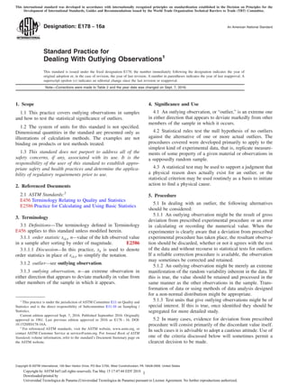
7.1.3 Example 1—As an illustration of the use of Tn and
Table 1, consider the following ten observations on breaking
strength (in pounds) of 0.104-in. hard-drawn copper wire: 568,
570, 570, 570, 572, 572, 572, 578, 584, 596. See Fig. 1. The
doubtful observation is the high value, x10 = 596. Is the value
of 596 significantly high? The mean is x¯ = 575.2 and the
estimated standard deviation is s = 8.70. We compute:
T10 5 ~596 2 575.2!/8.70 5 2.39 (3)
From Table 1, for n = 10, note that a T10 as large as 2.39
would occur by chance with probability less than 0.05. In fact,
so large a value would occur by chance not much more often
than 1 % of the time. Thus, the weight of the evidence is
against the doubtful value having come from the same popu-
lation as the others (assuming the population is normally
distributed). Investigation of the doubtful value is therefore
indicated.
7.2 Dixon Criteria for a Single Outlier—An alternative
system, the Dixon criteria (2),3
based entirely on ratios of
differences between the observations may be used in cases
where it is desirable to avoid calculation of s or where quick
judgment is called for. For the Dixon test, the sample criterion
or statistic changes with sample size. Table 2 gives the
appropriate statistic to calculate and also gives the critical
values of the statistic for the 1, 5, and 10 % levels of
significance. In most situations, the Dixon criteria is less
powerful at detecting an outlier than the criterion given in 7.1.
7.2.1 Example 2—As an illustration of the use of Dixon’s
test, consider again the observations on breaking strength given
in Example 1. Table 2 indicates use of:
r11 5 ~xn 2 x n21!/~xn 2 x2! (4)
Thus, for n = 10:
r11 5 ~x10 2 x 9!/~x10 2 x2! (5)
For the measurements of breaking strength above:
r11 5 ~596 2 584!/~596 2 570! 5 0.462 (6)
Which is a little less than 0.478, the 5 % critical value for n
= 10. Under the Dixon criterion, we should therefore not
consider this observation as an outlier at the 5 % level of
significance. These results illustrate how borderline cases may
be accepted under one test but rejected under another.
7.3 Recursive Testing for Multiple Outliers in Univariate
Samples—For testing multiple outliers in a sample, recursive
application of a test for a single outlier may be used. In
recursive testing, a test for an outlier, x1 or xn, is first
conducted. If this is found to be significant, then the test is
repeated, omitting the outlier found, to test the point on the
opposite side of the sample, or an additional point on the same
side. The performance of most tests for single outliers is
affected by masking, where the probability of detecting an
outlier using a test for a single outlier is reduced when there are
two or more outliers. Therefore, the recommended procedure is
to use a criterion designed to test for multiple outliers, using
recursive testing to investigate after the initial criterion is
significant.
7.4 Criterion for Two Outliers on Opposite Sides of a
Sample—In testing the least and the greatest observations
simultaneously as probable outliers in a sample, use the ratio of
sample range to sample standard deviation test of David,
Hartley, and Pearson (5):
w/s 5 ~x n 2 x1!/s (7)
The significance levels for this sample criterion are given in
Table 3. Alternatively, the largest residuals test of Tietjen and
Moore (7.5) could be used.
7.4.1 Example 3—This classic set consists of a sample of 15
observations of the vertical semidiameters of Venus made by
Lieutenant Herndon in 1846 (6). In the reduction of the
observations, Prof. Pierce found the following residuals (in
3
The boldface numbers in parentheses refer to a list of references at the end of
this standard.
TABLE 1 Critical Values for T (One-Sided Test) When Standard
Deviation is Calculated from the Same SampleA
Number of
Observations,
n
Upper 10 %
Significance
Level
Upper 5 %
Significance
Level
Upper 1 %
Significance
Level
3 1.1484 1.1531 1.1546
4 1.4250 1.4625 1.4925
5 1.602 1.672 1.749
6 1.729 1.822 1.944
7 1.828 1.938 2.097
8 1.909 2.032 2.221
9 1.977 2.110 2.323
10 2.036 2.176 2.410
11 2.088 2.234 2.485
12 2.134 2.285 2.550
13 2.175 2.331 2.607
14 2.213 2.371 2.659
15 2.247 2.409 2.705
16 2.279 2.443 2.747
17 2.309 2.475 2.785
18 2.335 2.504 2.821
19 2.361 2.532 2.854
20 2.385 2.557 2.884
21 2.408 2.580 2.912
22 2.429 2.603 2.939
23 2.448 2.624 2.963
24 2.467 2.644 2.987
25 2.486 2.663 3.009
26 2.502 2.681 3.029
27 2.519 2.698 3.049
28 2.534 2.714 3.068
29 2.549 2.730 3.085
30 2.563 2.745 3.103
35 2.628 2.811 3.178
40 2.682 2.866 3.240
45 2.727 2.914 3.292
50 2.768 2.956 3.336
A
Values of T are taken from Grubbs (1),3
Table 1. All values have been adjusted
for division by n – 1 instead of n in calculating s. Use Ref. (1) for higher sample
sizes up to n = 147.
FIG. 1 Ten Observations of Breaking Strength from Example 1
E178 − 16a

seconds of arc) which have been arranged in ascending order of
magnitude. See Fig. 2, above.
7.4.2 The deviations –1.40 and 1.01 appear to be outliers.
Here the suspected observations lie at each end of the sample.
The mean of the deviations is x¯ = 0.018, the standard deviation
is s = 0.551, and:
w/s 5 @1.01 2 ~21.40!#/0.551 5 2.41/0.551 5 4.374 (8)
From Table 3 for n = 15, we see that the value of w/s = 4.374
falls between the critical values for the 1 and 5 % levels, so if
the test were being run at the 5 % level of significance, we
would conclude that this sample contains one or more outliers.
7.4.3 The lowest measurement, –1.40, is 1.418 below the
sample mean, and the highest measurement, 1.01, is 0.992
above the mean. Since these extremes are not symmetric about
the mean, either both extremes are outliers, or else only –1.40
is an outlier. That –1.40 is an outlier can be verified by use of
the T1 statistic. We have:
T1 5 ~x¯ 2 x1!/s 5 @0.018 2 ~21.40!#/0.551 5 2.574 (9)
This value is greater than the critical value for the 5 % level,
2.409 from Table 1, so we reject –1.40. Since we have decided
that –1.40 should be rejected, we use the remaining 14
observations and test the upper extreme 1.01, either with the
criterion:
Tn 5 ~x n 2 x¯!/s (10)
or with Dixon’s r22. Omitting –1.40 and renumbering the
observations, we compute:
x¯ 5 1.67/14 5 0.119, s 5 0.401 (11)
and:
T14 5 ~1.01 2 0.119!/0.401 5 2.22 (12)
From Table 1, for n = 14, we find that a value as large as 2.22
would occur by chance more than 5 % of the time, so we
should retain the value 1.01 in further calculations. The Dixon
test criterion is:
r 22 5~x14 2 x12!/~x14 2 x3!
5~1.01 2 0.48!/~1.0110.24!
50.53/1.25
50.424
(13)
From Table 2 for n = 14, we see that the 5 % critical value
for r22 is 0.546. Since our calculated value (0.424) is less than
the critical value, we also retain 1.01 by Dixon’s test, and no
further values would be tested in this sample.
7.5 Criteria for Two or More Outliers on Opposite Sides of
the Sample—For suspected observations on both the high and
TABLE 2 Dixon Criteria for Testing of Extreme Observation (Single Sample)A
n Criterion
Significance Level (One-Sided Test)
10 % 5 % 1 %
3 r10 = (x2 − x1)/(xn − x1) if smallest value is suspected; 0.886 0.941 0.988
4 = (xn − xn−1)/(xn − x1) if largest value is suspected 0.679 0.766 0.889
5 0.558 0.642 0.781
6 0.484 0.562 0.698
7 0.434 0.507 0.637
8 r11 = (x2 − x1)/(xn−1 − x1) if smallest value is suspected; 0.480 0.554 0.681
9 = (xn − xn−1)/(xn − x2) if largest value is suspected. 0.440 0.511 0.634
10 0.410 0.478 0.597
13 0.467 0.521 0.617
16 0.453 0.505 0.598
17 0.437 0.489 0.580
18 0.424 0.475 0.564
19 0.412 0.462 0.550
20 0.401 0.450 0.538
21 0.391 0.440 0.526
22 0.382 0.430 0.516
23 0.374 0.421 0.506
24 0.366 0.413 0.497
25 0.359 0.406 0.489
26 0.353 0.399 0.482
27 0.347 0.393 0.474
28 0.342 0.387 0.468
29 0.336 0.381 0.462
30 0.332 0.376 0.456
35 0.311 0.354 0.431
40 0.295 0.337 0.412
45 0.283 0.323 0.397
50 0.272 0.312 0.384
A
x1 # x2 # ... # xn. Original Table in Dixon (2), Appendix. Critical values updated by calculations by Bohrer (3) and Verma-Ruiz (4).
FIG. 2 Fifteen Residuals from the Semidiameters of Venus from
Example 3
E178 − 16a

low sides in the sample, and to deal with the situation in which
some of k ≥ 2 suspected outliers are larger and some smaller
than the remaining values in the sample, Tietjen and Moore (7)
suggest the following statistic. Let the sample values be x1, x2,
x3, ..., xn. Compute the sample mean, x¯ , and the n absolute
residuals:
r1 5 ?x1 2 x¯?, r2 5 ?x2 2 x¯?, … , rn 5 ?xn 2 x¯? (14)
Now relabel the original observations x1, x2, ..., xn as z’s in
such a manner that zi is that x whose ri is the ith
smallest
absolute residual above. This now means that z1 is that
observation x which is closest to the mean and that zn is the
observation x which is farthest from the mean. The Tietjen-
Moore statistic for testing the significance of the k largest
residuals is then:
Ek 5 F(i51
n2k
~z i 2 z¯k! 2
/(i51
n
~zi 2 z¯! 2
G (15)
where:
z¯k 5 (i51
n2k
zi/~n 2 k! (16)
is the mean of the (n − k) least extreme observations and z¯ is
the mean of the full sample. Percentage points of Ek in Table 4
were computed by simulation.
7.5.1 Example 4—Applying this test to the Venus semidi-
ameter residuals data in Example 3, we find that the total sum
of squares of deviations for the entire sample is 4.24964.
Omitting –1.40 and 1.01, the suspected two outliers, we find
that the sum of squares of deviations for the reduced sample of
13 observations is 1.24089. Then E2 = 1.24089/4.24964 =
0.292, and by using Table 4, we find that this observed E2 is
slightly smaller than the 5 % critical value of 0.317, so that the
E2 test would reject both of the observations, –1.40 and 1.01.
7.6 Criterion for Two Outliers on the Same Side of the
Sample—Where the two largest or the two smallest observa-
tions are probable outliers, employ a test provided by Grubbs
TABLE 3 Critical ValuesA
(One-Sided Test) for w/s (Ratio of
Range to Sample Standard Deviation)
Number of
Observations,
n
10 %
Significance
Level
5 %
Significance
Level
1 %
Significance
Level
3 1.9973 1.9993 2.0000
4 2.409 2.429 2.445
5 2.712 2.755 2.803
6 2.949 3.012 3.095
7 3.143 3.222 3.338
8 3.308 3.399 3.543
9 3.449 3.552 3.720
10 3.574 3.685 3.875
11 3.684 3.803 4.011
12 3.782 3.909 4.133
13 3.871 4.005 4.244
14 3.952 4.092 4.344
15 4.025 4.171 4.435
16 4.093 4.244 4.519
17 4.156 4.311 4.597
18 4.214 4.374 4.669
19 4.269 4.433 4.736
20 4.320 4.487 4.799
21 4.368 4.539 4.858
22 4.413 4.587 4.913
23 4.456 4.633 4.965
24 4.497 4.676 5.015
25 4.535 4.717 5.061
26 4.572 4.756 5.106
27 4.607 4.793 5.148
28 4.641 4.829 5.188
29 4.673 4.863 5.226
30 4.704 4.895 5.263
35 4.841 5.040 5.426
40 4.957 5.162 5.561
45 5.057 5.265 5.674
50 5.144 5.356 5.773
A
Each entry calculated by 50 000 000 simulations.
TABLE 4 Tietjen-Moore Critical Values (One-Sided Test) for Ek
k 1A
2 3 4 5
n α 10 % 5 % 1 % 10 % 5 % 1 % 10 % 5 % 1 % 10 % 5 % 1 % 10 % 5 % 1 %
3 0.003 0.001 0.000 ... ... ... ... ... ... ... ... ... ... ... ...
4 0.049 0.025 0.004 0.002 0.001 0.000 ... ... ... ... ... ... ... ... ...
5 0.127 0.081 0.029 0.022 0.010 0.002 ... ... ... ... ... ... ... ... ...
6 0.203 0.145 0.068 0.056 0.034 0.012 0.009 0.004 0.001 ... ... ... ... ... ...
7 0.270 0.207 0.110 0.094 0.065 0.028 0.027 0.016 0.006 ... ... ... ... ... ...
8 0.326 0.262 0.156 0.137 0.099 0.050 0.053 0.034 0.014 0.016 0.010 0.004 ... ... ...
9 0.374 0.310 0.197 0.175 0.137 0.078 0.080 0.057 0.026 0.032 0.021 0.009 ... ... ...
10 0.415 0.353 0.235 0.214 0.172 0.101 0.108 0.083 0.044 0.052 0.037 0.018 0.022 0.014 0.006
11 0.451 0.390 0.274 0.250 0.204 0.134 0.138 0.107 0.064 0.073 0.055 0.030 0.036 0.026 0.012
12 0.482 0.423 0.311 0.278 0.234 0.159 0.162 0.133 0.083 0.094 0.073 0.042 0.052 0.039 0.020
13 0.510 0.453 0.337 0.309 0.262 0.181 0.189 0.156 0.103 0.116 0.092 0.056 0.068 0.053 0.031
14 0.534 0.479 0.374 0.337 0.293 0.207 0.216 0.179 0.123 0.138 0.112 0.072 0.086 0.068 0.042
15 0.556 0.503 0.404 0.360 0.317 0.238 0.240 0.206 0.146 0.160 0.134 0.090 0.105 0.084 0.054
16 0.576 0.525 0.422 0.384 0.340 0.263 0.263 0.227 0.166 0.182 0.153 0.107 0.122 0.102 0.068
17 0.593 0.544 0.440 0.406 0.362 0.290 0.284 0.248 0.188 0.198 0.170 0.122 0.140 0.116 0.079
18 0.610 0.562 0.459 0.424 0.382 0.306 0.304 0.267 0.206 0.217 0.187 0.141 0.156 0.132 0.094
19 0.624 0.579 0.484 0.442 0.398 0.323 0.322 0.287 0.219 0.234 0.203 0.156 0.172 0.146 0.108
20 0.638 0.594 0.499 0.460 0.416 0.339 0.338 0.302 0.236 0.252 0.221 0.170 0.188 0.163 0.121
25 0.692 0.654 0.571 0.528 0.493 0.418 0.417 0.381 0.320 0.331 0.298 0.245 0.264 0.236 0.188
30 0.730 0.698 0.624 0.582 0.549 0.482 0.475 0.443 0.386 0.391 0.364 0.308 0.325 0.298 0.250
35 0.762 0.732 0.669 0.624 0.596 0.533 0.523 0.495 0.435 0.443 0.417 0.364 0.379 0.351 0.299
40 0.784 0.756 0.704 0.657 0.629 0.574 0.562 0.534 0.480 0.486 0.458 0.408 0.422 0.395 0.347
45 0.802 0.776 0.728 0.684 0.658 0.607 0.593 0.567 0.518 0.522 0.492 0.446 0.459 0.433 0.386
50 0.820 0.796 0.748 0.708 0.684 0.636 0.622 0.599 0.550 0.552 0.529 0.482 0.492 0.468 0.424
A
From Grubbs (8),Table 1, for n # 25.
E178 − 16a

(8, 9) which is based on the ratio of the sample sum of squares
when the two doubtful values are omitted to the sample sum of
squares when the two doubtful values are included. In illus-
trating the test procedure, we give the following Examples 5
and 6.
7.6.1 It should be noted that the critical values in Table 5 for
the 1 % level of significance are smaller than those for the 5 %
level. So for this particular test, the calculated value is
significant if it is less than the chosen critical value.
7.6.2 Example 5—In a comparison of strength of various
plastic materials, one characteristic studied was the percentage
elongation at break. Before comparison of the average elonga-
tion of the several materials, it was desirable to isolate for
further study any pieces of a given material which gave very
small elongation at breakage compared with the rest of the
pieces in the sample. Ten measurements of percentage elonga-
tion at break made on a material are: 3.73, 3.59, 3.94, 4.13,
3.04, 2.22, 3.23, 4.05, 4.11, and 2.02. See Fig. 3. Arranged in
ascending order of magnitude, these measurements are: 2.02,
2.22, 3.04, 3.23, 3.59, 3.73, 3.94, 4.05, 4.11, 4.13.
7.6.2.1 The questionable readings are the two lowest, 2.02
and 2.22. We can test these two low readings simultaneously
by using the S1,2
2
/S2
criterion of Table 5. For the above
measurements:
S2
5 Σ
i51
n
~xi 2 x¯!2
5 5.351
S1,2
2
5 Σ
i53
n
~x 2 x¯1,2!2
5 1.196, where x¯1,2 5 Σ
i53
n
xi ⁄~n 2 2!
S1,2
2
⁄S2
5 1.197⁄5.351 5 0.2237
From Table 5 for n = 10, the 5 % significance level for
S1,2
2
/S2
is 0.2305. Since the calculated value is less than the
critical value, we should conclude that both 2.02 and 2.22 are
outliers. In a situation such as the one described in this
example, where the outliers are to be isolated for further
analysis, a significance level as high as 5 % or perhaps even 10
% would probably be used in order to get a reasonable size of
sample for additional study.
7.6.3 Example 6—The following ranges (horizontal dis-
tances in yards from gun muzzle to point of impact of a
projectile) were obtained in firings from a weapon at a constant
angle of elevation and at the same weight of charge of
propellant powder. The distances arranged in increasing order
of magnitude are:
4420 4782
4549 4803
4730 4833
4765 4838
7.6.3.1 It is desired to make a judgment on whether the
projectiles exhibit uniformity in ballistic behavior or if some of
the ranges are inconsistent with the others. The doubtful values
are the two smallest ranges, 4420 and 4549. For testing these
two suspected outliers, the statistic S1,2
2
/S2
is used. The value
of S2
is 158592. Omission of the two shortest ranges, 4420 and
4549, and recalculation, gives S1,2
2
equal to 8590.8. Thus:
S1,2⁄S2
5 8590.8⁄158592 5 0.0542 (17)
which is significant at the 0.01 level (see Table 5). It is thus
highly unlikely that the two shortest ranges (occurring actually
from excessive yaw) could have come from the same popula-
tion as that represented by the other six ranges. It should be
noted that the critical values in Table 5 for the 1 % level of
significance are smaller than those for the 5 % level. So for this
particular test, the calculated value is significant if it is less
than the chosen critical value.
NOTE 2—Kudo (10) indicates that if the two outliers are due to a shift
in location or level, as compared to the scale σ, then the optimum sample
criterion for testing should be of the type:
min (2 – xi – xj)/s = (2 – x1 – x2)/s in Example 5.
7.7 Criteria for Two or More Outliers on the Same Side of
the Sample—An extension of the S1,2
2
⁄S2
criterion is given by
Tietjen and Moore (7). Percentage points for the k ≥ 2 highest
or lowest sample values are given in Table 6, where:
Lk 5 (i51
n2k
~xi 2 x¯k! 2
/(i51
n
~x i 2 x¯! 2
and x¯k 5 (i51
n2k
xi/~n 2 k!
NOTE 3—For k = 1, L1 is equivalent to the statistic Tn for a single
outlier. For k = 2, L2 equals Sn, n21
2
⁄S2
.
7.8 Skewness and Kurtosis Criteria—When several outliers
are present in the sample, the detection of one or two spurious
values may be “masked” by the presence of other anomalous
TABLE 5 Critical Values for S2
n− 1, n / S2
, or S2
1,2 / S2
for
Simultaneously Testing the Two Largest or Two Smallest
ObservationsA
Number of
Observations, n
Lower 10 %
Significance
Level
Lower 5 %
Significance
Level
Lower 1 %
Significance
Level
4 0.0031 0.0008 0.0000
5 0.0376 0.0183 0.0035
6 0.0920 0.0564 0.0186
7 0.1479 0.1020 0.0440
8 0.1994 0.1478 0.0750
9 0.2454 0.1909 0.1082
10 0.2863 0.2305 0.1414
11 0.3227 0.2667 0.1736
12 0.3552 0.2996 0.2043
13 0.3843 0.3295 0.2333
14 0.4106 0.3568 0.2605
15 0.4345 0.3818 0.2859
16 0.4562 0.4048 0.3098
17 0.4761 0.4259 0.3321
18 0.4944 0.4455 0.3530
19 0.5113 0.4636 0.3725
20 0.5270 0.4804 0.3909
21 0.5415 0.4961 0.4082
22 0.5550 0.5107 0.4245
23 0.5677 0.5244 0.4398
24 0.5795 0.5373 0.4543
25 0.5906 0.5495 0.4680
26 0.6011 0.5609 0.4810
27 0.6110 0.5717 0.4933
28 0.6203 0.5819 0.5050
29 0.6292 0.5916 0.5162
30 0.6375 0.6008 0.5268
35 0.6737 0.6405 0.5730
40 0.7025 0.6724 0.6104
45 0.7261 0.6985 0.6412
50 0.7459 0.7203 0.6672
A
From Grubbs (1), Table II. An observed ratio less than the appropriate critical
ratio in this table calls for rejection of the null hypothesis.
FIG. 3 Ten Measurements of Percentage Elongation at Break
from Example 5
E178 − 16a

observations. So far we have discussed procedures for detect-
ing a fixed number of outliers in the same sample, but these
techniques are not generally the most sensitive. Sample skew-
ness and kurtosis are defined in Practice E2586. They are
commonly used to test normality of a distribution, but may also
be used as outlier tests. Outlying observations occur due to a
shift in level (or mean), or a change in scale (that is, change in
variance of the observations), or both. For several outliers and
repeated rejection of observations, the sample coefficient of
skewness:
g1 5
nΣ~xi 2 x¯!3
~n 2 1!~n 2 2!s3
should be used to test against change in level of several
observations in the same direction, and the sample coefficient
of kurtosis:
g2 5
n~n 1 1!Σ~xi 2 x¯!4
~n 2 1!~n 2 2!~n 2 3!s4 2
3~n 2 1!2
~n 2 2!~n 2 3!
is recommended to test against change in level to both higher
and lower values and also for changes in scale (variance).
7.8.1 In applying the above tests, g1 or g2, or both, are
computed and if their observed values exceed those for
significance levels given in Tables 7 and 8, then the observa-
tion farthest from the mean is rejected and the same procedure
repeated until no further sample values are judged as outliers.
Critical values in Tables 7 and 8 were obtained by simulation.
7.8.2 Ferguson (11, 12) studied the power of the various
rejection rules relative to changes in level or scale. The g1
statistic has the optimum property of being “locally” best
against an alternative of shift in level (or mean) in the same
direction for multiple observations. g2 is similarly locally best
against alternatives of shift in both directions, or a of a change
in scale for several observations. The g1 test is good for up to
50 % spurious observations in the sample for the one-sided
case, and the g2 test is optimum in the two-sided alternatives
case for up to 21 % “contamination” of sample values. For only
one or two outliers the sample statistics of the previous
TABLE 6 Tietjen-Moore Critical Values (One-Sided Test) for Lk
k 1A
2B
3 4 5
n α 10 % 5 % 1 % 10 % 5 % 1 % 10 % 5 % 1 % 10 % 5 % 1 % 10 % 5 % 1 %
3 0.011 0.003 0.000 ... ... ... ... ... ... ... ... ... ... ... ...
4 0.098 0.049 0.010 0.003 0.001 0.000 ... ... ... ... ... ... ... ... ...
5 0.199 0.127 0.044 0.038 0.018 0.004 ... ... ... ... ... ... ... ... ...
6 0.283 0.203 0.093 0.092 0.056 0.019 0.020 0.010 0.002 ... ... ... ... ... ...
7 0.350 0.270 0.145 0.148 0.102 0.044 0.056 0.032 0.010 ... ... ... ... ... ...
8 0.405 0.326 0.195 0.199 0.148 0.075 0.095 0.064 0.028 0.038 0.022 0.008 ... ... ...
9 0.450 0.374 0.241 0.245 0.191 0.108 0.134 0.099 0.048 0.068 0.045 0.018 ... ... ...
10 0.488 0.415 0.283 0.286 0.230 0.141 0.170 0.129 0.070 0.098 0.070 0.032 0.051 0.034 0.012
11 0.520 0.451 0.321 0.323 0.267 0.174 0.208 0.162 0.098 0.128 0.098 0.052 0.074 0.054 0.026
12 0.548 0.482 0.355 0.355 0.300 0.204 0.240 0.196 0.120 0.159 0.125 0.070 0.103 0.076 0.038
13 0.573 0.510 0.386 0.384 0.330 0.233 0.270 0.224 0.147 0.186 0.150 0.094 0.126 0.098 0.056
14 0.594 0.534 0.414 0.411 0.357 0.261 0.298 0.250 0.172 0.212 0.174 0.113 0.150 0.122 0.072
15 0.613 0.556 0.440 0.435 0.382 0.286 0.322 0.276 0.194 0.236 0.197 0.132 0.172 0.140 0.090
16 0.631 0.576 0.463 0.456 0.405 0.310 0.342 0.300 0.219 0.260 0.219 0.151 0.194 0.159 0.108
17 0.646 0.593 0.485 0.476 0.426 0.332 0.364 0.322 0.237 0.282 0.240 0.171 0.216 0.181 0.126
18 0.660 0.610 0.504 0.494 0.446 0.353 0.384 0.337 0.260 0.302 0.259 0.192 0.236 0.200 0.140
19 0.673 0.624 0.522 0.511 0.464 0.373 0.398 0.354 0.272 0.316 0.277 0.211 0.251 0.217 0.154
20 0.685 0.638 0.539 0.527 0.480 0.391 0.420 0.377 0.300 0.339 0.299 0.231 0.273 0.238 0.175
25 0.732 0.692 0.607 0.591 0.550 0.468 0.489 0.450 0.377 0.412 0.374 0.308 0.350 0.312 0.246
30 0.766 0.730 0.650 0.637 0.601 0.527 0.523 0.506 0.434 0.472 0.434 0.369 0.411 0.376 0.312
35 0.792 0.762 0.690 0.674 0.641 0.573 0.586 0.554 0.484 0.516 0.482 0.418 0.458 0.424 0.364
40 0.812 0.784 0.722 0.702 0.673 0.610 0.622 0.588 0.522 0.554 0.523 0.460 0.499 0.468 0.408
45 0.826 0.802 0.745 0.726 0.698 0.641 0.648 0.618 0.558 0.586 0.556 0.498 0.533 0.502 0.444
50 0.840 0.820 0.768 0.746 0.720 0.667 0.673 0.646 0.592 0.614 0.588 0.531 0.562 0.535 0.483
A
From Grubbs (8), Table I for n# 25.
B
From Grubbs (1), Table II.
TABLE 7 Significance LevelsA
(One-Sided Test) for Skewness g1
Number of
Observations,
n
10 %
Significance
Level
5 %
Significance
Level
1 %
Significance
Level
3 1.647 1.711 1.731
4 1.439 1.709 1.940
5 1.224 1.564 1.994
6 1.090 1.428 1.959
7 1.014 1.320 1.886
8 0.956 1.246 1.813
9 0.903 1.183 1.735
10 0.862 1.131 1.668
11 0.828 1.086 1.610
12 0.798 1.049 1.556
13 0.770 1.011 1.504
14 0.744 0.977 1.461
15 0.722 0.950 1.418
16 0.702 0.922 1.379
17 0.684 0.899 1.345
18 0.667 0.875 1.310
19 0.651 0.856 1.281
20 0.636 0.836 1.252
21 0.624 0.818 1.225
22 0.610 0.800 1.196
23 0.599 0.786 1.175
24 0.587 0.770 1.150
25 0.578 0.757 1.132
26 0.567 0.743 1.108
27 0.558 0.731 1.091
28 0.549 0.718 1.070
29 0.541 0.708 1.056
30 0.532 0.695 1.036
35 0.497 0.649 0.965
40 0.467 0.610 0.904
45 0.442 0.578 0.853
50 0.422 0.551 0.812
A
E178 − 16a

paragraphs are recommended, and Ferguson (11) discusses in
detail their optimum properties of pointing out one or two
outliers.
7.8.3 Example 7—For the elongation at break data (Ex-
ample 5), the value of skewness is g1 = –0.969. From Table 7
with n = 10, and taking into account that the two lowest values
are the suspected outliers, the 5 % significance value is –1.131,
with skewness less than this value being significant. The
skewness test does not conclude that there are outliers in this
case.
7.8.4 Example 8—The kurtosis test is applied to the Venus
semidiameter residuals data of Example 3 to test the highest
and lowest values. The value of kurtosis for the 15 observations
is g2 = 2.528. The 5 % significance value from Table 8 is 2.145.
Using this test, we conclude that at least one of the values is an
outlier. With the value on the low side, –1.40, removed, the
value of skewness is g1
= 0.767. The 5 % significance value
from Table 7 is 0.977, so no further outliers are concluded.
8. Recommended Criterion Using an Independent
Standard Deviation
8.1 Suppose that an independent estimate of the standard
deviation is available from previous data. This estimate may be
from a single sample of previous similar data or may be the
result of combining estimates from several such previous sets
of data. When one uses an independent estimate of the standard
deviation, sv, the test criterion for an outlier is as follows:
T'1 5 ~x¯ 2 x1!/sv (18)
or:
T'n 5 ~x n 2 x¯!/sv (19)
where:
v = total number of degrees of freedom.
8.2 Critical values for T1' and Tn' given by David (13) are in
Table 9. In Table 9 the subscript v = df indicates the total
number of degrees of freedom associated with the independent
estimate of standard deviation σ and n indicates the number of
observations in the sample under study.
8.3 A slight over-approximation to critical values of T1' and
Tn' is based on the Student’s t distribution:
Tn
'
~α! # tα⁄n,v=1 2 1⁄n
where tα/n,v is the upper α/n percentage point of Student’s t
distribution with v degrees of freedom.
8.4 The population standard deviation σ may be known
accurately. In such cases, Table 10 may be used for single
outliers.
9. Additional Comments: Reinforcement and New Issues
9.1 The presence or lack of outliers is determined using
statistical testing on the basis of an underlying assumed normal
distribution in this practice. Some additional remarks and
alternative approaches are noted.
9.2 If the mathematical form of the underlying uncontami-
nated statistical distribution is known and not normal or
transformable to normal, for example, an exponential life
distribution, then outlier testing should specifically account for
it. Some classes of data provide distributions that are highly
asymmetric (skewed).
9.3 In general, the more is known about data variation, the
better a position the experimenter is in to test for outliers.
Outlier tests provided can be classified based on availability of
prior information on variation: nothing known (Tables 1 and
2), limited historical information (Table 9), standard deviation
known (Table 10). A cautionary note is that a historical
variation estimate must still be relevant.
9.4 Much outlier practice is directed towards a more reliable
estimate of a measure of the mean. If a goal of study is instead
to make inferences about variability or to estimate a relatively
low or high quantile of the distribution, then any action that is
taken with the disposition of perceived outliers dramatically
changes the resulting statistical estimates and interpretation.
9.5 All of the documented test methodologies are univari-
ate. This practice does not address the issue of multivariate
outlier testing or testing in time-ordered or structured data.
9.6 The outlier tests provided in this practice are generally
most useful with moderate numbers of observations. Outlier
tests that only use information about variability internal to the
sample can only reject gross outlying values. With much larger
numbers of observations, especially in data sets that have not
been screened by a knowledgeable reviewer to remove invalid
observations, the presence of invalid data is to be expected.
The statistical basis for the tests in the previous sections, that
TABLE 8 Significance LevelsA
for Kurtosis g2
Number of
Observations,
n
10 %
Significance
Level
5 %
Significance
Level
1 %
Significance
Level
4 3.075 3.518 3.900
5 2.772 3.506 4.454
6 2.482 3.319 4.685
7 2.257 3.110 4.735
8 2.067 2.935 4.687
9 1.904 2.772 4.586
10 1.778 2.627 4.467
11 1.678 2.505 4.350
12 1.597 2.399 4.234
13 1.529 2.300 4.106
14 1.471 2.217 4.000
15 1.422 2.145 3.887
16 1.378 2.081 3.784
17 1.340 2.021 3.702
18 1.303 1.966 3.605
19 1.271 1.921 3.524
20 1.243 1.873 3.450
21 1.214 1.831 3.370
22 1.188 1.788 3.298
23 1.167 1.757 3.233
24 1.143 1.719 3.169
25 1.123 1.690 3.116
26 1.102 1.658 3.051
27 1.085 1.630 2.995
28 1.066 1.601 2.943
29 1.052 1.578 2.903
30 1.035 1.550 2.845
35 0.969 1.446 2.642
40 0.913 1.358 2.470
45 0.867 1.285 2.322
50 0.830 1.223 2.210
A
E178 − 16a

there should be a low probability of rejecting any value if the
distribution is normal, is less compelling in that case.
9.7 Alternative Outlier Procedures—Outlier rejection rules
based on robust statistical measure have been introduced. The
Tukey boxplot rule (Practice E2586) rejects values more than
a multiple (1.5) of the interquartile range from the lower or
upper quartile of a data set. Hampel’s rule rejects values that
are farther than a multiple (4.5 or 5.2) of the median absolute
deviation away from the median of the data set. The commonly
used rejection criteria for each were still selected to provide a
reasonable signiﬁcance level(s) for an assumed underlying
uncontaminated normal distribution.
9.8 Outlier Accommodation—Robust statistical methods are
insensitive to small numbers of outlier data. Examples are use
of the median or trimmed mean as estimates of the mean, and
least absolute deviations for regression. Many robust estima-
tion methods have been developed, but have not yet gained the
TABLE 9 Critical Values (One-Sided Test) for T' When Standard Deviation s v is Independent of Present SampleA
T' 5
xn 2 x¯
sv
, or
x¯ 2 x 1
sv
v = d.f.
n
3 4 5 6 7 8 9 10 12
1 % signiﬁcance level
10 2.78 3.10 3.32 3.48 3.62 3.73 3.82 3.90 4.04
11 2.72 3.02 3.24 3.39 3.52 3.63 3.72 3.79 3.93
12 2.67 2.96 3.17 3.32 3.45 3.55 3.64 3.71 3.84
13 2.63 2.92 3.12 3.27 3.38 3.48 3.57 3.64 3.76
14 2.60 2.88 3.07 3.22 3.33 3.43 3.51 3.58 3.70
15 2.57 2.84 3.03 3.17 3.29 3.38 3.46 3.53 3.65
16 2.54 2.81 3.00 3.14 3.25 3.34 3.42 3.49 3.60
17 2.52 2.79 2.97 3.11 3.22 3.31 3.38 3.45 3.56
18 2.50 2.77 2.95 3.08 3.19 3.28 3.35 3.42 3.53
19 2.49 2.75 2.93 3.06 3.16 3.25 3.33 3.39 3.50
20 2.47 2.73 2.91 3.04 3.14 3.23 3.30 3.37 3.47
24 2.42 2.68 2.84 2.97 3.07 3.16 3.23 3.29 3.38
30 2.38 2.62 2.79 2.91 3.01 3.08 3.15 3.21 3.30
40 2.34 2.57 2.73 2.85 2.94 3.02 3.08 3.13 3.22
60 2.29 2.52 2.68 2.79 2.88 2.95 3.01 3.06 3.15
120 2.25 2.48 2.62 2.73 2.82 2.89 2.95 3.00 3.08
` 2.22 2.43 2.57 2.68 2.76 2.83 2.88 2.93 3.01
10 2.01 2.27 2.46 2.60 2.72 2.81 2.89 2.96 3.08
11 1.98 2.24 2.42 2.56 2.67 2.76 2.84 2.91 3.03
12 1.96 2.21 2.39 2.52 2.63 2.72 2.80 2.87 2.98
13 1.94 2.19 2.36 2.50 2.60 2.69 2.76 2.83 2.94
14 1.93 2.17 2.34 2.47 2.57 2.66 2.74 2.80 2.91
15 1.91 2.15 2.32 2.45 2.55 2.64 2.71 2.77 2.88
16 1.90 2.14 2.31 2.43 2.53 2.62 2.69 2.75 2.86
17 1.89 2.13 2.29 2.42 2.52 2.60 2.67 2.73 2.84
18 1.88 2.11 2.28 2.40 2.50 2.58 2.65 2.71 2.82
19 1.87 2.11 2.27 2.39 2.49 2.57 2.64 2.70 2.80
20 1.87 2.10 2.26 2.38 2.47 2.56 2.63 2.68 2.78
24 1.84 2.07 2.23 2.34 2.44 2.52 2.58 2.64 2.74
30 1.82 2.04 2.20 2.31 2.40 2.48 2.54 2.60 2.69
40 1.80 2.02 2.17 2.28 2.37 2.44 2.50 2.56 2.65
60 1.78 1.99 2.14 2.25 2.33 2.41 2.47 2.52 2.61
120 1.76 1.96 2.11 2.22 2.30 2.37 2.43 2.48 2.57
` 1.74 1.94 2.08 2.18 2.27 2.33 2.39 2.44 2.52
10 1.68 1.92 2.09 2.23 2.33 2.42 2.50 2.56 2.68
11 1.66 1.90 2.07 2.20 2.30 2.39 2.46 2.53 2.64
12 1.65 1.88 2.05 2.17 2.28 2.36 2.44 2.50 2.61
13 1.63 1.86 2.03 2.16 2.26 2.34 2.41 2.47 2.58
14 1.62 1.85 2.01 2.14 2.24 2.32 2.39 2.45 2.56
15 1.61 1.84 2.00 2.12 2.22 2.31 2.38 2.44 2.54
16 1.61 1.83 1.99 2.11 2.21 2.29 2.36 2.42 2.52
17 1.60 1.82 1.98 2.10 2.20 2.28 2.35 2.41 2.51
18 1.59 1.82 1.97 2.09 2.19 2.27 2.34 2.39 2.49
19 1.59 1.81 1.96 2.08 2.18 2.26 2.33 2.38 2.48
20 1.58 1.80 1.96 2.08 2.17 2.25 2.32 2.37 2.47
24 1.57 1.78 1.94 2.05 2.15 2.22 2.29 2.34 2.44
30 1.55 1.77 1.92 2.03 2.12 2.20 2.26 2.32 2.41
40 1.54 1.75 1.90 2.01 2.10 2.17 2.23 2.29 2.38
60 1.52 1.73 1.87 1.98 2.07 2.14 2.20 2.26 2.35
120 1.51 1.71 1.85 1.96 2.05 2.12 2.18 2.23 2.32
` 1.50 1.70 1.83 1.94 2.02 2.09 2.15 2.20 2.28
A
The percentage points are reproduced from Ref. (13).
E178 − 16a

wide use to be considered standard replacements for the
customary least squares methods.
9.9 Additional literature and monographs that summarize a
range of viewpoints on the detection and handling of outliers
are listed in Refs. (9, 11, 14-19).
10. Keywords
10.1 Dixon test; gross deviation; Grubbs test; kurtosis;
outlier; skewness; Tietjen-Moore test
REFERENCES
(1) Grubbs, F. E., and Beck, G., “Extension of Sample Sizes and
Percentage Points for Significance Tests of Outlying Observations,”
Technometrics, TCMTA, Vol 14, No. 4, November 1972, pp. 847–854.
(2) Dixon, W. J., “Processing Data for Outliers,” Biometrics, BIOMA, Vol
9, No. 1, March 1953, pp. 74–89.
(3) Bohrer, A., “One-sided and Two-sided Critical Values for Dixon’s
Outlier Test for Sample Sizes up to n=30,” Economic Quality Control,
Vol 23, No. 1, 2008, pp. 5–13.
(4) Verma, S. P., and Quiroz-Ruiz, A., “Critical Values for Six Dixon
Tests for Outliers in Normal Samples up to Sizes 100, and Applica-
tions in Science and Engineering,” Revista Mexicana de Ciencias
Geologicas, Vol 23, No. 2, 2006, pp. 133–161.
(5) David, H. A., Hartley, H. O., and Pearson, E. S., “The Distribution of
the Ratio, in a Single Normal Sample, of Range to Standard
Deviation,” Biometrika, BIOKA, Vol 41, 1954, pp. 482–493.
(6) Chauvenet, W., Method of Least Squares, Lippincott, Philadelphia,
1868.
(7) Tietjen, G. L., and Moore, R. H., “Some Grubbs-Type Statistics for
the Detection of Several Outliers,” Technometrics, TCMTA, Vol 14,
No. 3, August 1972, pp. 583–597. Corrigendum Technometrics, Vol
21, No. 3, August 1979, p. 396.
(8) Grubbs, F. E., “Sample Criteria for Testing Outlying Observations,”
Annals of Mathematical Statistics, AASTA, Vol 21, March 1950, pp.
27–58.
(9) Grubbs, F. E., “Procedures for Detecting Outlying Observations in
Samples,” Technometrics, TCMTA, Vol 11, No. 4, February 1969, pp.
1–21.
(10) Kudo, A., “On the Testing of Outlying Observations,” Sankhya, The
Indian Journal of Statistics, SNKYA, Vol 17, Part 1, June 1956, pp.
67–76.
(11) Ferguson, T. S., “On the Rejection of Outliers,” Fourth Berkeley
Symposium on Mathematical Statistics and Probability, edited by
Jerzy Neyman, University of California Press, Berkeley and Los
Angeles, Calif., 1961.
(12) Ferguson, T. S., “Rules for Rejection of Outliers,” Revue Inst. Int. de
Stat., RINSA, Vol 29, No. 3, 1961, pp. 29–43.
(13) David, H. A., “Revised Upper Percentage Points of the Extreme
Studentized Deviate from the Sample Mean,” Biometrika, BIOKA,
Vol 43, 1956, pp. 449–451.
(14) Anscombe, F. J.,“Rejection of Outliers,” Technometrics, TCMTA,
Vol 2, No. 2, 1960, pp. 123–147.
(15) Barnett, V., “The Study of Outliers: Purpose and Model,” Applied
Statistics, Vol 27, 1978, pp. 242–250.
(16) Hawkins, D. M., Identification of Outliers, Chapman and Hall,
London, 1980.
(17) Beckman, R. J., and Cook, R. D., “Outlier……….s,” Technometrics,
Vol 25, No. 2, 1983, pp. 119–149.
(18) Iglewicz, B., and Hoaglin, D. C., How to Detect and Handle
Outliers, ASQ Quality Press, 1993.
(19) Barnett, V. and Lewis, T., Outliers in Statistical Data, 3rd ed., John
Wiley and Sons, Inc., New York, 1995.
TABLE 10 Critical ValuesA
(One-Sided Test) of T'1` and T'n` When
the Population Standard Deviation σ is Known
Number of 10 % 5 % 1 %
Observations, Significance Significance Significance
n Level Level Level
2 1.163 1.386 1.822
3 1.497 1.737 2.216
4 1.696 1.941 2.431
5 1.834 2.080 2.574
6 1.939 2.184 2.679
7 2.022 2.266 2.761
8 2.091 2.334 2.827
9 2.149 2.392 2.884
10 2.200 2.441 2.932
11 2.245 2.485 2.973
12 2.284 2.523 3.009
13 2.320 2.558 3.042
14 2.352 2.589 3.072
15 2.382 2.618 3.099
16 2.409 2.644 3.124
17 2.434 2.668 3.147
18 2.458 2.691 3.168
19 2.480 2.712 3.187
20 2.500 2.732 3.206
21 2.520 2.750 3.223
22 2.538 2.768 3.240
23 2.556 2.785 3.255
24 2.572 2.800 3.270
25 2.588 2.815 3.284
26 2.602 2.829 3.297
27 2.617 2.844 3.310
28 2.631 2.857 3.322
29 2.644 2.869 3.334
30 2.656 2.881 3.345
35 2.712 2.935 3.395
40 2.760 2.980 3.437
45 2.801 3.019 3.472
50 2.837 3.054 3.504
A
E178 − 16a

ASTM International takes no position respecting the validity of any patent rights asserted in connection with any item mentioned
in this standard. Users of this standard are expressly advised that determination of the validity of any such patent rights, and the risk
of infringement of such rights, are entirely their own responsibility.
This standard is subject to revision at any time by the responsible technical committee and must be reviewed every ﬁve years and
if not revised, either reapproved or withdrawn. Your comments are invited either for revision of this standard or for additional standards
and should be addressed to ASTM International Headquarters. Your comments will receive careful consideration at a meeting of the
responsible technical committee, which you may attend. If you feel that your comments have not received a fair hearing you should
make your views known to the ASTM Committee on Standards, at the address shown below.
This standard is copyrighted by ASTM International, 100 Barr Harbor Drive, PO Box C700, West Conshohocken, PA 19428-2959,
United States. Individual reprints (single or multiple copies) of this standard may be obtained by contacting ASTM at the above
address or at 610-832-9585 (phone), 610-832-9555 (fax), or service@astm.org (e-mail); or through the ASTM website
(www.astm.org). Permission rights to photocopy the standard may also be secured from the Copyright Clearance Center, 222
Rosewood Drive, Danvers, MA 01923, Tel: (978) 646-2600; http://www.copyright.com/
E178 − 16a

E178.13738

Recommended

Recommended

More Related Content

What's hot

What's hot (20)

Similar to E178.13738

Similar to E178.13738 (20)

Recently uploaded

Recently uploaded (20)

E178.13738