1. Chapter 2
Elementary Cam Lift Curve Synthesis
Abstract This chapter describes the derivation and piece-wise integration of the
first half of an analytically simple valve acceleration curve. Two simultaneous
algebraic equations are obtained. The first equates an expression for the velocity
on the nose of the cam to zero, and the second the sum of the increments of valve
lift to the maximum specified lift. The two unknowns are the maximum positive
acceleration, which is on the flank of the cam and the maximum negative accel-
eration, which is on the nose of the cam. The two equations can then be solved for
these two unknown quantities. This example has been chosen for analytical sim-
plicity, to demonstrate the method, but such an acceleration curve would not result
is a good cam design with smooth valve acceleration, and should not be used in
practice. A superior and useable, but analytically more complex acceleration curve
is considered in the next chapter.
2.1 Introduction
Some of the concepts of cam lift curve synthesis were described in Chap. 1.
Over the years many methods of obtaining the acceleration diagram have been
used and the method described below and refined in Chap. 3 is only one of these.
The example given here has been chosen for its analytical simplicity, but this
type of acceleration curve should not be used in practice, as it is not a good one.
It has been said that misconceptions tend to harden into axioms, and the simple
example given below is based on a method which was surprisingly still being used
by at least one company for cam design in the early 1980s. The use of some cams
designed with especially rapid changes in acceleration, or jerk, resulted in con-
siderable valve spring surge and consequent spring failures, which then resulted in
destruction of much of the engine. However, despite the difficulties in synthesising
J. J. Williams, Introduction to Analytical Methods for Internal Combustion Engine 31
Cam Mechanisms, DOI: 10.1007/978-1-4471-4564-6_2, Ó Springer-Verlag London 2013

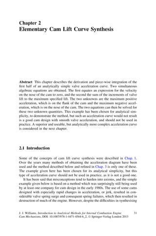
2. 32 2 Elementary Cam Lift Curve Synthesis
acceptably smooth cam lift curves before the advent of digital computers, they
were produced and used, but this was very time consuming.
The use of cams exhibiting significant jerk with push rod mechanisms or
other mechanisms subject to relatively flexible behaviour can result in a loss of
cam–follower contact, which will impair reliability and power output. This sort
of cam will also be far more likely to induce valve spring surge in otherwise
stiffer mechanisms which apart from valve spring failure will again result in a
loss of cam–follower contact at a lower engine speed. Unstable behaviour of the
cam mechanism may lead to valve clash, damage to the piston, valve and valve
seat, or loss of power due to poor gas flow, or a combination of these unde-
sirable effects.
2.2 An Elementary Cam Lift Curve
The cam lift curve is obtained by designing an acceleration curve and then inte-
grating to obtain a velocity curve and then a lift curve. It is convenient to divide
the curve into two parts, the opening half and a closing half. These two parts meet
on the nose, and at this point the curves need to be smoothly continuous. In fact we
shall require them to be continuously differentiable.
For this initial example it is helpful to consider a curve with few components
and consisting of analytically simple sections, with discontinuous rates of change
of acceleration. A more realistic example is considered later, but this has more
sections and is more complicated and the amount of algebra involved tends to
mask the basic method.
When the engine is assembled it is necessary to specify a tappet clearance, s0 , to
allow for thermal expansion of the valve stem when the engine is at working
temperature. If there were no initial clearance then the valve would not be closed,
when the tappet was touching the cam’s base circle. It is necessary to take up this
initial clearance as smoothly as possible, and one solution might be to have a ramp
of length, T0 , linearly increasing lift to a height of s0 at T0 .
Derivatives with respect to time are denoted in this chapter using Newton’s
dot notation. The slope of this ramp, s0 , would then be, given by: s0 ¼ s0 =T0 .
_ _
_
Unfortunately, this results in an instantaneous change in the velocity, s0 , which
would require an infinite acceleration for an infinitesimally small time, as
described in Sect. 1.2.1. This, so-called Delta function, would not be realised in
practice but such a ramp design is best avoided, as the jerk needs to be as small
as possible. For this initial example let the ramp have a constant acceleration, A0 ,
as shown in Fig. 2.1. The notional tappet clearance, s0 , is specified by the
designer.

3. 2.2 An Elementary Cam Lift Curve 33
Fig. 2.1 An elementary
Acceleration
acceleration diagram
A
T3
A0 T4 T
0 T0 T1 T2
F
2.2.1 Notation
A Maximum acceleration
"
A Parameter defined in text
^
A Parameter defined in text
A0 Initial ramp height
^
A0 Parameter defined in text
F Maximum deceleration
^
F Parameter defined in text
L Maximum lift
s Lift
s0 Lift at end of ramp, tappet clearance
t Time
T Time interval
2.2.2 An Elementary Acceleration Curve
After the initial ramp the next three sections are linear and the final section consists
of a quarter sine wave. Although this would not be an acceptable design in
practice, it will permit a minimum of mathematics and will therefore be easier to
follow the method. By splitting the acceleration curve into sections and integrating
twice we can obtain two equations in two unknowns, A and F. At T4 the velocity is
zero and the valve lift, L, is specified by the designer. The slope of the acceleration
v
curve at T4 is s4 ¼ 0.
The acceleration curve shown in Fig. 2.1 has discontinuities in slope at
0; T0 ; T1 ; T2 and T3 , which cause large instantaneous changes in the rate of change

4. 34 2 Elementary Cam Lift Curve Synthesis
of acceleration or jerk. This will lead to surging and premature failure of metallic
coil valve-springs, and a tendency for instabilities in the motion of cam mecha-
nisms with low elastic stiffness such as those involving push-rods. At very high
camshaft speeds, even stiff mechanisms with pneumatic valve springs can have a
tendency to behave in an unstable manner, if there are significantly large values of
jerk. There is also insufficient flexibility to permit the designer to optimise his
design, and the use of a section which is a quarter sine-wave will not allow the
energy stored in the spring to be used efficiently to maintain contact between
follower and cam; this limits the maximum engine speed that can safely be used
before contact is lost between cam and tappet.
By considering each section in turn the equation for the acceleration is inte-
grated twice and the constants of integration determined from the initial boundary
conditions for each section.
Constant Acceleration Ramp. 0 t T0 ; 0 T T0
With notation of Fig. 2.1:
Integrating Eq. (2.1) twice w.r.t. t:
€ ¼ A0
s ð2:1Þ
s ¼ A0 t
_ ð2:2Þ
A0 t 2
s¼ ð2:3Þ
2
At t ¼ T0 :
€ ¼ €0 ¼ A0
s s ð2:4Þ
s 0 ¼ A0 T 0
_ ð2:5Þ
2
A0 T0
s ¼ s0 ¼ ð2:6Þ
2
Hence:
2s0
A0 ¼ 2
ð2:7Þ
T0
As s0 and T0 are specified by the designer, A0 can be determined.
Linearly Increasing Acceleration. T0 t T1 ; T0 T T1
ðA À A0 Þt
€ ¼ A0 þ
s ð2:8Þ
T1
Integrating Eq. (2.8) twice w.r.t. t:

5. 2.2 An Elementary Cam Lift Curve 35
ðA À A0 Þt2
s ¼ s 0 þ A0 t þ
_ _ ð2:9Þ
2T1
A0 t2 ðA À A0 Þt3
s ¼ s0 þ s0 t þ
_ þ ð2:10Þ
2 6T1
At t ¼ T1 :
€ ¼ €1 ¼ A
s s ð2:11Þ
A0 T1 AT1
s ¼ s1 ¼ s0 þ
_ _ _ þ ð2:12Þ
2 2
2 2
A0 T1 AT1
s ¼ s1 ¼ s0 þ s0 T1 þ
_ þ ð2:13Þ
3 6
Constant Acceleration. T1 t T2 ; T1 T T2
€¼A
s ð2:14Þ
Integrating Eq. (2.14) twice w.r.t. t:
s ¼ s1 þ At
_ ð2:15Þ
At2
s ¼ s1 þ s1 t þ
_ ð2:16Þ
2
At t ¼ T2 :
€ ¼ €2 ¼ A
s s ð2:17Þ
s ¼ s2 ¼ s1 þ AT2
_ _ _ ð2:18Þ
2
AT2
s ¼ s2 ¼ s1 þ s1 T2 þ
_ ð2:19Þ
2
Linearly Decreasing Acceleration. T2 t T3 ; T2 T T3
t
€¼A 1À
s ð2:20Þ
T3
Integrating Eq. (2.19) twice w.r.t. t:
t2
s ¼ s2 þ A t À
_ _ ð2:21Þ
2T3

6. 36 2 Elementary Cam Lift Curve Synthesis
t2 t3
s ¼ s2 þ st þ A
_ À ð2:22Þ
2 6
At t ¼ T3 :
€3 ¼ 0
s ð2:23Þ
AT3
s3 ¼ s2 þ
_ _ ð2:24Þ
2
2
AT3
s3 ¼ s2 þ s2 T3 þ
_ ð2:25Þ
3
Sinusoidal Deceleration. T3 t T4 ; T3 T T4
pt
€ ¼ ÀF sin
s ð2:26Þ
2T4
Integrating Eq. (2.25) twice w.r.t.t:
!
2T4 pt
s ¼ s3 À F
_ _ 1 À cos ð2:27Þ
p 2T4
2 !
2T4 pt pt
s ¼ s3 þ s3 t À F
_ À sin ð2:28Þ
p 2T4 2T4
At t ¼ T4 :
€4 ¼ ÀF
s ð2:29Þ
The velocity on the nose is zero therefore:
2FT4
s4 ¼ s3 À
_ _ ¼0 ð2:30Þ
p
The maximum lift is specified by the designer hence:
4T4 p
2
s4 ¼ s3 þ s3 T4 À F
_ À1 ¼L ð2:31Þ
p2 2
_
Solution of Equations for A and F. The equations for s4 and s4 have two
unknowns, A and F. By substituting Eqs. (2.5), (2.12), and (2.18) into Eq. (2.30)
and after some algebra, we can write:
! !
T1 T1 þ T3 2FT4
s4 ¼ A0 T0 þ
_ þA þ T2 À ¼0 ð2:32Þ
2 2 p

7. 2.2 An Elementary Cam Lift Curve 37
Let:
0 ¼ A0 T0 þ T1
A ð2:33Þ
2
and
T1 þ T3
A¼ þ T2 ð2:34Þ
2
Substituting Eqs. (2.6), (2.13) and (2.19) into (2.33) together with Eqs. (2.5),
(2.12) and (2.18) into Eq. (2.32), and after further lengthy back substitutions and
algebra, we can write:
!
T2 T 2 T1
s4 ¼ A0 0 þ T0 ðT1 þ T2 þ T3 þ T4 Þ þ 1 þ ðT2 þ T3 þ T4 Þ
2 3 2
2 2 2
!
T T T T1 T3 T4
A 1 þ 2 þ 3 þ ðT2 þ T3 þ T4 Þ þ T2 ðT3 þ T4 Þ þ ð2:35Þ
6 2 3 2 2
4T 2 p
À F 24 À1 ¼L
p 2
Let:
!
^ T2 T 2 T1
A0 ¼ A0 0 þ T0 ðT1 þ T2 þ T3 þ T4 Þ þ 1 þ ðT2 þ T3 þ T4 Þ ð2:36Þ
2 3 2
and
!
^ T 2 T 2 T 2 T1 T3 T4
A ¼ A 1 þ 2 þ 3 þ ðT2 þ T3 þ T4 Þ þ T2 ðT3 þ T4 Þ þ ð2:37Þ
6 2 3 2 2
When simplifying lengthy algebraic equations, it is helpful to equate some
expressions to new parameters. This makes the analysis simpler to follow and
when writing computer code this makes for shorter expressions and reduces coding
errors. By considering the individual increments of the equations the simplification
process can be made more easily which results in less likelihood of terms being
missed and errors made. The method given below may not be necessary for the
present example, but is used in Chap. 3 where the acceleration diagram is more
complex.
From Eq. (2.5):
A
dV0 0 ¼ A0 T0 ð2:38Þ
From Eq. (2.6):
2
A0 T0
dSA0 ¼
0 ð2:39Þ
2

8. 38 2 Elementary Cam Lift Curve Synthesis
From Eq. (2.12):
A A0 T1
dV1 0 ¼ ð2:40Þ
2
A AT1
dV1 ¼ ð2:41Þ
2
A
dV1
dv1 ¼ ð2:42Þ
A
From Eq. (2.13):
2
A0 T1
dSA0 ¼
1 ð2:43Þ
3
2
AT1
dSA ¼
1 ð2:44Þ
6
dS1
ds1 ¼ ð2:45Þ
A
From Eq. (2.18):
dV2 ¼ AT2 ð2:46Þ
dV2
dv2 ¼ ð2:47Þ
A
From Eq. (2.19):
2
AT2
dS2 ¼ ð2:48Þ
2
dS2
ds2 ¼ ð2:49Þ
A
From Eq. (2.24):
AT3
dV3 ¼ ð2:50Þ
2
dV3
dv3 ¼ ð2:51Þ
A
From Eq. (2.25):
2
AT3
dS3 ¼ ð2:52Þ
3
dS2
ds2 ¼ ð2:53Þ
A

9. 2.2 An Elementary Cam Lift Curve 39
From Eq. (2.30):
À2FT4
dV4 ¼ ð2:54Þ
p
dV4
dv4 ¼ ð2:55Þ
F
From Eq. (2.31):
À4FT4 p
2
dS4 ¼ À1 ð2:56Þ
p2 2
dS4
ds4 ¼ ð2:57Þ
F
Let:
A A
RV A0 ¼ V0 0 þ V1 0 ð2:58Þ
Let:
RV A ¼ Aðdv1 þ dv2 þ dv3 Þ ð2:59Þ
Let:
RSA0 ¼ dSA0 þ dSA0 þ dV0 0 ðT1 þ T2 þ T3 þ T4 Þ þ dV1 0 ðT2 þ T3 þ T4 Þ ð2:60Þ
0 1
A A
Let:
 Ã
RSA ¼ A dsA þ dsA þ dsA þ dvA ðT2 þ T3 þ T4 Þ þ dvA ðT3 þ T4 Þ þ dvA T4
1 2 3 1 2 3
ð2:61Þ
Equation (2.30) can be written as:
2FT4
s4 ¼ RV A0 þ RV A À
_ ð2:62Þ
p
Equation (2.31) can be written as:
4FT4 p
2
S4 ¼ RSA0 þ RSA À 2
À1 ð2:63Þ
p 2
Evaluation of Eqs. (2.59) and (2.60) confirm Eqs. (2.37) and (2.38):
A0
RV ¼ A 0 ¼ A0 T0 þ T1 ð2:64Þ
2
T 1 þ T3
RV A ¼ A ¼ þ T2 ð2:65Þ
2

10. 40 2 Elementary Cam Lift Curve Synthesis
Evaluation of Eqs. (2.66) and (2.67) confirm Eqs. (2.37) and (2.38):
!
A0 ^ T2 T 2 T1
RS ¼ A0 ¼ A0 0 þ T0 ðT1 þ T2 þ T3 þ T4 Þ þ 1 þ ðT2 þ T3 þ T4 Þ
2 3 2
ð2:66Þ
2 2 2
!
^ T1 T2 T3 T1 T3 T4
RSA ¼ A ¼ A þ þ þ ðT2 þ T3 þ T4 Þ þ T2 ðT3 þ T4 Þ þ ð2:67Þ
6 2 3 2 2
Substituting Eqs. (2.33) and (2.34) into Eq. (2.32):
2FT4
s 4 ¼ A0 þ AA À
_ ¼0 ð2:32Þ
p
pðA0 þ AAÞ
F¼ ð2:68Þ
2T4
Substituting Eqs. (2.36) and (2.37) into Eq. (2.35):
^ ^ 4T4 p
2
s4 ¼ A0 þ AA À F 2
À1 ¼L ð2:69Þ
p 2
Hence:
^ ^ pðA0 þ AAÞ 4T4 p
2
A A ¼ L À A0 þ À1 ð2:70Þ
2T4 p2 2
Let:
^ 2T4 p À 1
F¼ ð2:71Þ
p 2
From Eqs. (2.70) and (2.71):
^ ^
L À A0 þ F A0
A¼ ð2:72Þ
^ ^
A À FA
 À ÁÃ
^ ^
p A0 þ A L À A þ F A0
F¼ À Á ð2:73Þ
^ ^
2T4 A À AF
Having solved these equations for the parameters A and F, we can compute the
lift velocity, and acceleration for each section of each curve. When initially
checking a program the velocity on the nose should be identically zero and the
computed maximum lift should agree with the specified value.
The parameters acceleration, velocity and lift can then be obtained for each
section of the curve in turn using a new loop for each section. Other errors in the
program may be found by checking that the values of the parameters give con-
tinuous curves at the joints between sections. Any discontinuities will indicate
where to look for an error.

11. http://www.springer.com/978-1-4471-4563-9