SlideShare a Scribd company logo
1 of 52
Download to read offline
A review of some plasticity and viscoplasticity
constitutive theories
J.L. Chaboche
ONERA DMSM, 29 Avenue de la Division Leclerc, BP72 F-92322 Châtillon Cedex, France
University of Technology of Troyes, LASMIS, 12 rue Marie Curie, 10010 Troyes, France
a r t i c l e i n f o
Article history:
Received 1 October 2007
Received in final revised form
14 March 2008
Available online 14 April 2008
Keywords:
Continuum mechanics
Plasticity
Viscoplasticity
Strain hardening
Ratchetting
a b s t r a c t
The purpose of the present review article is twofold:
 recall elementary notions as well as the main ingredients and
assumptions of developing macroscopic inelastic constitutive
equations, mainly for metals and low strain cyclic conditions.
The explicit models considered have been essentially developed
by the author and co-workers, along the past 30 years;
 summarize and discuss a certain number of alternative theoreti-
cal frameworks, with some comparisons made with the previous
ones, including more recent developments that offer potential
new capabilities.
Ó 2008 Elsevier Ltd. All rights reserved.
1. Introduction
The constitutive equation of the material is an essential ingredient of any structural calculation. It
provides the indispensable relation between the strains and the stresses, which is a linear relation in
the case of elastic analyses (Hooke’s law) and a much more complex nonlinear relation in inelastic
analyses, involving time and additional internal variables.
In this paper we limit ourselves to considering the conventional ‘‘Continuum” approach, i.e. that
the Representative Volume Element (RVE) of material is considered as subject to a near-uniform mac-
roscopic stress. This Continuum assumption is equivalent to neglecting the local heterogeneity of the
stresses and strains within the RVE, working with averaged quantities, as the effects of the heteroge-
neities act only indirectly through a certain number of ‘‘internal variables.” Moreover, in the frame-
work of the ‘‘local state” assumption of Continuum Thermomechanics, it is considered that the
0749-6419/$ - see front matter Ó 2008 Elsevier Ltd. All rights reserved.
doi:10.1016/j.ijplas.2008.03.009
E-mail address: Jean-Louis.Chaboche@onera.fr
International Journal of Plasticity 24 (2008) 1642–1693
Contents lists available at ScienceDirect
International Journal of Plasticity
journal homepage: www.elsevier.com/locate/ijplas
state of a material point (and of its immediate vicinity in the sense of the RVE) is independent of that
of the neighboring material point. Therefore the stress strain gradients do not enter into the
constitutive equations. This assumption is obviously questioned in recent theories of Generalized Con-
tinuum Mechanics, that are not addressed here.
The entire presentation will be limited to quasi-static movements considered to be slow enough, in
the framework of small perturbations (small strains of less than 10%, for example). Also, the equations
indicated will be formulated without explicitly stating the effect of temperature (although this may be
very large in certain cases). In other words, in accordance with the common practice for determining
the constitutive equations of solid materials, we will assume the temperature is constant (and uniform
over the RVE). The effect of the temperature will come into play only by the change of the ‘‘material”
parameters defining the constitutive equations. Moreover, the above mentioned Continuum Thermo-
dynamic framework will not be considered in detail. Only a few remarks are made as consequences of
such a theoretical framework for the temperature rate effect in the hardening rules.
The presentation is more directly oriented toward metallic type materials with elasto-plastic or
elasto-viscoplastic properties even though, in a way, viscoelasticity, i.e. the effect of viscosity on elas-
ticity, could be modeled from a viscoplastic model. Among the effects considered, we will thus have:
irreversible strain, or plastic strain, the associated phenomena of strain hardening, the time effects,
whether they enter by the effect of the loading velocity or through slow time variations of the various
variables (static recovery, for example). Aging phenomena (associated with possible changes in the
metallurgical structure) and damage effects will be mentioned only briefly. The anelasticity of the
metals (very low viscous hysteresis in the ‘‘elastic” range), which corresponds to reversible motions
of the dislocations, will not be discussed either. Only initially isotropic materials are considered, in
which anisotropy is the result of plastic flow and associated hardening processes.
In the present paper, the presentation of constitutive equations is made by following an increasing
order of complexity. It can essentially be considered in two parts:
 half the paper addresses to readers who are not too much informed about the plasticity/viscoplas-
ticity framework. It is more or less an introduction to unified viscoplastic constitutive models,
mainly based on the works made around the author;
 the second part considers more elaborated aspects, reviewing some other unified viscoplastic con-
stitutive theories, pointing out some similarities and differences. Other constitutive frameworks are
also discussed. The present capabilities of the various kinematic hardening models are compared in
the context of predicting ratchetting effects, including modified Armstrong–Frederick based rules as
well as multi-surface and two-surface theories.
A special mention here about the Armstrong–Frederick Report (Armstrong and Frederick, 1966)
that serves of common basis for many kinematic hardening rules. This work was never published, only
available as a Technical Report from CEGB (Central Electricity Generating Board). By using this rule in
the context of unified viscoplasticity and generalising it continuously, the author contributed to the
knowledge and citation of this report. In 2007, it has been published in ‘‘Materials at High Tempera-
ture”, accompanied with a Preface retracing this story (Frederick and Armstrong, 2007).
Let us point out that the review of existing modelling methodologies in the context of cyclic plas-
ticity and viscoplasticity cannot be at all exhaustive. We hope only to provide the indispensable gen-
eral elements, as well as the main types of modelling. The interested reader should refer to more
complete specialized works (Lemaître and Chaboche, 1985; Khan and Huang, 1995; Franc
ßois et al.,
1991; Miller, 1987b; Krauss and Krauss, 1996; Besson et al., 2001).
2. Basic notions
The general context of modelling the inelastic behaviour in rate-independent plasticity or in visco-
plasticity is supposed to be known, as being sufficiently standard. Many more details and interesting
exercises on this current and standard framework can be found in textbooks, like in Khan and Huang
(1995). Only the main assumptions and equations are indicated and briefly commented here, as they
could be necessary for understanding further developments in the paper.
J.L. Chaboche / International Journal of Plasticity 24 (2008) 1642–1693 1643
We assume the small strain framework. This is justified by the domain of application to cyclic load-
ing conditions. The main equations are given below, considering also isothermal conditions. The first
equation defines the partition of total strain tensor into an elastic strain and a plastic strain, though
the second one gives corresponding Hooke’s Law of linear elasticity.
e

¼ e

e
þ e

p
ð1Þ
r

¼ L

: ðe

e

p
Þ ð2Þ
f ¼ k r

 X

kH  k 6 0 ð3Þ
_
e

p
¼ _
k
of
o r

¼ _
k n

ð4Þ
An aside on the notations: the symbol ‘‘.” between two tensors designates the product contracted once
((rikrkj ¼ r2
ij with Einstein’s summation, represents the square of the tensor r

); the symbol ‘‘:” desig-
nates the product contracted twice (for example the scalar rijrji ¼ Trr

2
).
In the framework of rate-independent plasticity, we need the use of an elasticity domain, f 6 0, as
given by (3). The yield surface f ¼ 0 is defined in (3) with Hill’s criterion, using a fourth rank tensor H

within a quadratic norm definition as
k r

kH ¼
ffiffiffiffiffiffiffiffiffiffiffiffiffiffiffiffiffiffiffi
r

: H

: r

r
ð5Þ
More sophisticated yield surface or loading surface definitions could be used. Examples can be found
in recent works by Cazacu and Barlat (2004) or Barlat et al. (2007), but will not be considered in the
present review.
In Eq. (3) parameter k is the initial yield surface size. Moreover, hardening induced by plastic flow is
assumed to be described by a combination of kinematic hardening and isotropic hardening. We use
the back-stress X

for kinematic hardening and the increase of yield surface size R for the isotropic
hardening.
Figs. 1 and 2 illustrate, in the deviatoric stress plane and in the uniaxial tension–compression par-
ticular case, the transformation of the elastic domain and yield surface by the two particular cases of
pure isotropic hardening and pure linear kinematic hardening.
In what follows we also assume the associated plasticity framework (the flow potential is identical
with the yield surface) and the normality law (4) expresses the consequence of the maximum dissi-
pation principle. In the rate-independent framework, the plastic multiplier _
k is determined by the con-
sistency condition f ¼ _
f ¼ 0.
In case of a viscoplastic behaviour (or rate dependency), the above plasticity framework is general-
ized by using a viscoplastic potential Xðf Þ. The stress state goes beyond the elasticity domain with a
Fig. 1. Schematics of the isotropic hardening. Left: in the deviatoric plane; right: the stress vs plastic strain response.
1644 J.L. Chaboche / International Journal of Plasticity 24 (2008) 1642–1693
positive value of rv ¼ f  0, that can be called the viscous stress, or the overstress. In that case, nor-
mality rule reads:
_
e

p
¼
oXðfÞ
o r

¼
oX
of
of
o r

¼ _
p
of
o r

¼ _
p n

ð6Þ
_
k is replaced by _
p, the norm of the viscoplastic strain rate, as defined by
_
p ¼ k_
e

p
kH1 ð7Þ
Therefore, p is the length of the plastic strain path in the plastic strain space.
Let us conclude this brief introduction of the general framework by indicating the particular case
where orthotropic Hill’s criterion is restricted to von Mises one, with
H

¼
3
2
I

d
¼
3
2
I


1
3
1

 1

 
ð8Þ
where I

and I

d
are respectively the fourth rank unit tensor and deviatoric projector. In such case, von
Mises elastic domain is given by
f ¼ k r

 X

k  R  k ¼
ffiffiffiffiffiffiffiffiffiffiffiffiffiffiffiffiffiffiffiffiffiffiffiffiffiffiffiffiffiffiffiffiffiffiffiffiffiffiffiffiffiffiffiffiffi
3
2
ðr

0  X

0Þ : ðr

0  X

0Þ
s
 R  k 6 0 ð9Þ
where r

0
and X

0
are deviatoric parts, like r

0
¼ r

 1
3
Trr1

. Correspondingly, the direction of the plastic
strain rate is
_
e

p
¼
oX
o r

¼ _
p
3
2
r

0
 X

0
k r

 X

k
¼ _
p n

ð10Þ
The accumulated plastic strain rate then writes
_
p ¼
ffiffiffiffiffiffiffiffiffiffiffiffiffiffiffiffiffi
2
3
_
e

p : _
e

p
s
ð11Þ
Let us note that, the yield surface being independent on the first stress invariant, plastic flow does not
induce a volume change (Tr _
ep
¼ 0, n

: n

¼ 3=2). Moreover, any stress state can be broken down into
the following form, in which the function rvð_
pÞ is deduced by inversion of the relation _
p ¼ oX=of.
r

¼ X

þðR þ k þ rvð_
pÞÞ n

ð12Þ
3. Unified theory of viscoplasticity
To simplify the discussion, we adopt the viscoplasticity scheme directly. The case of rate-indepen-
dent plasticity will be deduced from this as a limiting case. We begin by giving a rather general form to
Fig. 2. Schematics of the linear kinematic hardening. Left: in the deviatoric plane; right: the stress vs plastic strain response.
J.L. Chaboche / International Journal of Plasticity 24 (2008) 1642–1693 1645
the constitutive equations, and then we examine the most common particular options, for the viscos-
ity function and for the isotropic and kinematic hardening. The main ingredients in the theory are ta-
ken from the unified constitutive model of the author (Chaboche, 1977b). Various other versions will
be discussed in Section 5. We then examine the case of rate-independent plasticity and finish with a
few indications on determining the parameters of the equations from experiments.
3.1. General form of the constitutive equation
Let us point out right away that this can be established in the general formal framework of contin-
uum thermodynamics. This subject will not be addressed here. The interested reader can refer to Ger-
main (1973), Halphen and Nguyen (1975), Chaboche (1996), for example.
The expression for the viscoplastic constitutive equation essentially includes two aspects:
 the choice of the viscosity function (see Section 3.2), or choice of the viscoplastic potential X, which
will act in the expression for the viscoplastic strain rate (its dependency on the viscous stress)
through the normality Eq. (6) stated above;
 the choice of the hardening equations for all of the internal variables. These are provisionally denoted
aj ðj ¼ 1; 2; . . . ; NÞ, which can be scalar or tensorial. The general form includes a strain hardening
term, a dynamic recovery term, and a static recovery term:
_
aj ¼ hjð  Þ_
ep
 rD
j ð  Þaj _
ep
 rS
j ð. . .Þaj ð13Þ
The first term gives an (increasing) evolution of aj with the plastic strain. The second, on the other
hand, gives a recall, or evanescent memory effect; but this acts again (instantaneously) with the plas-
tic strain, whence the dynamic recovery term. The third term is called static recovery or time recovery,
or thermal recovery, since it can act independently of any plastic strain. This is very clear in an incre-
mental statement such that da ¼ hdep  rD
adep  rS
adt. The functions hj; rD
j ; rS
j are to be defined (see
below). Let us note right away that the static recovery mechanism is ‘‘thermally activated” and that
the effect of the temperature in the function rS
j plays an essential role. Roughly speaking, this terms
is used to express the effects of the thermal agitation, inducing dislocation climbing mechanisms
and the corresponding annihilation possibility, or even recrystallization effects in certain cases. Let
us also indicate a strong analogy with equations of physical origin in Garofalo (1965), Kocks (1976),
Estrin and Mecking (1984), concerning the dislocation density q, for example according to Estrin
(1996) in uniaxial loading:
dq ¼ Mðko þ k1
ffiffiffiffi
q
p
 k2qÞdep  rS
ð
ffiffiffiffi
q
p
; TÞdt ð14Þ
3.2. Choice of the viscosity function
This relation between the viscous stress and the plastic strain rate norm is usually highly nonlinear.
Thus, through a large range of velocities, it can be approximated by a power function:
_
p ¼
f
D
 n
¼
rv
D
D En
ð15Þ
The McCauley brackets hi are used here to ensure that when f  0, i.e. inside the elastic domain, _
p can-
cels out continuously. This expression corresponds to Norton’s equation (or Odqvist’s law in three-
dimensional context) for the secondary creep, when the hardening is neglected. Exponent n depends
on the material, on the strain rate domain considered, and on the temperature, ranging from a theo-
retical value of n ¼ 1 for the ‘‘diffusional creep” of a perfect alloy to sometimes very high values when
we approach the material’s low viscosity range (at low temperatures). In practice, it is usually ob-
served that 3 6 n 6 30 for current engineering materials.
The advantage of expression (15) is that it easily derives from the viscoplastic potential:
X ¼
D
n þ 1
rv
D
D Enþ1
ð16Þ
1646 J.L. Chaboche / International Journal of Plasticity 24 (2008) 1642–1693
For certain materials, an effect of saturation of the rate effect can be felt in the high rate regime. Fig. 3
shows the example of 316L stainless steel at 550 °C. The intermediate velocity range, where the rela-
tion between log10rv and log10 _
ep appears to be approximately linear with a slope of n ¼ 24, extends to
low rates by a rapid drop in the stress (due to static recovery phenomena that will be studied further
on) and by a stress saturation at high velocities between 103
and 101
s1
. Various expressions may
be proposed to express such a saturation effect in the viscosity function. They are studied and com-
pared in Section 5.7.
3.3. Isotropic hardening equations
When we consider the expression for the norm of the strain rate (15), by replacing f with (9), we
find:
_
p ¼
k r

 X

k  R  k
D
* +n
ð17Þ
We find three possibilities for introducing a hardening of the isotropic type:
(i) through the variable R, by an increase in the size of the elasticity domain,
(ii) by increase of the drag stress D,
(iii) by coupling with the evolution law of the kinematic hardening variable X

.
In the first two cases, the only ones considered here, we just have to define the one-to-one relation-
ship between R (or D) and the state variable of the isotropic hardening, which is the accumulated plas-
tic strain p (or possibly the accumulated plastic work Wp).
R ¼ RðpÞ D ¼ DðpÞ ð18Þ
One possibility among others is to let the two evolutions be ‘‘proportional.” We can then define only
the function RðpÞ and deduce from it
DðpÞ ¼ K þ fRðpÞ ð19Þ
where K is the initial value of the drag stress and f is a weighting parameter. One special case, corre-
sponding to the Perzyna (1964) approach, is the one obtained with K ¼ k and f ¼ 1.
By decomposition of the equivalent von Mises stress (in the case without kinematic hardening,
X

¼ 0), we can note the different roles of the two types of isotropic hardening
req ¼ k þ RðpÞ þ rvð_
p; pÞ ¼ k þ RðpÞ þ DðpÞ_
p1=n
ð20Þ
Fig. 3. Overstress vs plastic strain rate on 316 L Stainless Steel at 600 °C, and its interpretation with the double slope and
exponential functions.
J.L. Chaboche / International Journal of Plasticity 24 (2008) 1642–1693 1647
In the first case, with R, the elastic domain will be increased in the same way whatever the strain rate.
In the second, the increase in D will cause an increase in req that will be greater with greater strain
rate. The simplest and most used form of viscoplasticity equation with isotropic hardening is the
one that is deduced from the combination of the secondary creep law (Norton’s law with a power
function between the secondary creep rate and the applied stress) and the primary creep law (power
relation between strain and time). Such approaches may be found in Rabotnov (1969), Lemaître
(1971). It is equivalent to neglecting, in (17) any elasticity domain ðk ¼ 0Þ, the corresponding harden-
ing RðpÞ, and adopting a power function for the drag stress D. This would be expressed:
req ¼ Kp1=m
_
p1=n
ð21Þ
This multiplicative form of the work hardening is very practical to determine (Lemaître, 1971) and
yields good results in a rather large domain, at least for quasi-proportional monotonic loadings.
3.4. Kinematic hardening equations
As kinematic type of hardening is a nearly general occurrence, at least in the range of moderate
strains, the corresponding models will have to be used when we want to correctly express either
non-proportional monotonic loadings (variation of the loading direction, thermomechanical loadings,
etc.), or cyclic loadings.
The most widespread kinematic hardening models are indicated here in increasing order of com-
plexity. A few more advanced models for expressing special effects can be found in Sections 7 and
8. For the time being, we are discussing only strain hardening, while the time recovery effects are con-
sidered in Section 3.7.
The simplest model is Prager’s linear kinematic hardening (Prager, 1949), in which the evolution of
the kinematic variable X

(called back-stress) is collinear with the evolution of the plastic strain. Thus
_
X

¼
2
3
C _
e

p
and X

¼
2
3
Ce

p
ð22Þ
The linearity associated with the stress–strain response (Fig. 2-b) is rarely observed (except perhaps in
the regime of significant strains). A better description is given by the model proposed initially by Arm-
strong and Frederick (1966)1
introducing a recall term, called dynamic recovery:
_
X

¼
2
3
C _
e

p
 cX

_
p ð23Þ
The recall term is collinear with X

(as in the general Eq. (13)) and is proportional to the norm of the
plastic strain rate. The evolution of X

, instead of being linear, is then exponential for a monotonic uni-
axial loading, with a saturation for a value C=c. That is, the integration of (23) with respect to ep, for a
uniaxial loading, yields:
X ¼ m
C
c
þ Xo  m
C
c
 
expðmcðep  epo
ÞÞ ð24Þ
in which m ¼ 1 gives the flow direction and where X0 and ep0
are the values of X and ep at the begin-
ning of the loading branch considered.
For strain-controlled cyclic loading, it is shown that the stabilization occurs when Xmax þ Xmin ¼ 0:
DX
2
¼ jXoj ¼
C
c
tanh c
Dep
2
 
ð25Þ
Fig. 4 gives the example of a few materials, treated in the rate-independent case, in which the cyclic
curve is described with (25) and Dr
2
¼ DX
2
þ k.
1
Interesting to note: this work was never published, only available as a Technical Report from CEGB (Central Electricity
Generating Board). By using this rule in the context of unified viscoplasticity and generalising it continuously, the author
contributed to the knowledge and citation of this report. In 2007, it has been published in ‘‘Materials at High Temperature”,
accompanied with a Preface retracing this story (Frederick and Armstrong, 2007).
1648 J.L. Chaboche / International Journal of Plasticity 24 (2008) 1642–1693
A better approximation, given in Chaboche et al. (1979), Chaboche and Rousselier (1983), consists
in adding several models such as (23), with significantly different recall constants ci (factors from 5 to
20 between each of them):
X

¼
X
M
i¼1
X
i
_
X

i
¼
2
3
Ci _
e

p
 ciX
i _
p ð26Þ
allowing the expression of a more extensive strain domain and a better description of the soft transi-
tion between elasticity and the onset of plastic flow. Fig. 4 shows, for 35NCD16 hard steel, the signif-
icant improvement in the case where only two variables are superposed, one being linear, with c2 ¼ 0.
Let us note here that the number of parameters introduced by such a superposition of back-stresses
(set of fci; Cig) should not be considered as material parameters but as a series decomposition of a sim-
pler expression of the tensile curve (or cyclic curve), for instance by a power law. This has been proved
later by Watanabe and Atluri (1986), based on the endochronic theory of Valanis (1980).
Other more complex combinations can be used (Cailletaud and Saï, 1995) instead of (26), but they
do not allow analytical closed form solutions in uniaxial loading. In Section 7 we will also indicate var-
ious modifications of the basic AF rule used above, especially in order to improve plastic ratchetting
predictions by the constitutive models.
3.5. Cyclic hardening–softening
In the framework of kinematic hardening models, isotropic hardening is generally used to express
the cyclic evolution of the material’s mechanical strength with respect to the plastic flow. This cyclic
hardening phenomenon (increase of strength) or cyclic softening (decrease) is relatively slow, typi-
cally taking between ten and a thousand cycles of ep ¼ 0:2%, for example, before stabilizing.
We can control the dimension of the elasticity domain with a law of the type:
_
R ¼ bðQ  RÞ_
p ð27Þ
which is the direct transposition of (23) to isotropic hardening, with b and Q being two coefficients
depending on the material and on the temperature (b will be included between 50 and 0.5 to ensure
the typical saturation mentioned above in 10 and 1000 cycles, respectively). The integration of (27)
leads to an expression RðpÞ ¼ Qð1  expðbpÞÞ that can also be used in the context of monotonic load-
ings (but a much higher value is then needed for b).
Fig. 4. Cyclic curves on various materials and their interpretation by the AF rule or the multikinematic model.
J.L. Chaboche / International Journal of Plasticity 24 (2008) 1642–1693 1649
Fig. 5, reproduced from Goodall et al. (1980), shows the example of 316 Stainless Steel, using a nor-
malised plot of the maximum stress evolution as a function of the accumulated plastic strain:
rM  rM0
rMS
 rM0
¼ 1  expðbpÞ ð28Þ
where rM is the current maximum stress, rM0
and rMS
being the corresponding initial (1st cycle) and
stabilised values. The figure shows the validity of the choice (27) because the normalised experimental
responses are approximately independent on the plastic strain range, as the model assumes.
Let us note that, in the case of cyclic softening, we can set Q  0, so that the stabilised yield surface
size k þ Q will be lower than the initial one (R is assumed to be the change in the size, usually with
Rð0Þ ¼ 0. Also note that the drag stress D can be used in place of the yield stress R, or the two can
be combined, or a coupling can be introduced between the kinematic hardening and isotropic harden-
ing (Marquis, 1979) with a function /ðpÞ to be defined
_
X

i
¼
2
3
Ci _
e

p
 ci/ðpÞX
i _
p ð29Þ
Fig. 6 illustrates the case of 316 SS with the function / defined as / ¼ /1 þ ð1  /1Þ expðbpÞ. It
shows a slight dependency on the plastic strain range but not in contradiction with experimental
results.
Another possible choice of /ðpÞ consists in using the variable R with a dependency deduced from an
endochronic type theory (Valanis, 1980; Watanabe and Atluri, 1986):
/ðpÞ ¼ 1=ð1 þ xRðpÞÞ ð30Þ
Remark. Let us recall here, without more details, that endochronic theory of plasticity developed by
Valanis (1980) is one based on the hereditary form of thermodynamics of irreversible processes,
though the present formulations are developed in the context of thermodynamics with internal
variables (Germain, 1973). See a few more details in Section 4.1.2. Such hereditary theories, like in
viscoelasticity, uses the complete history of observable variables (strain and temperature), without
using the notion of internal variables. This is done by integral equation to relate stress and strain
tensors histories, which kernel contains most phenomenological information. This is the case for
instance with the theory developed in France by Guélin and co-workers (Guélin and Stutz, 1977;
Boisserie et al., 1983).
It is interesting to underline here the following fact: as demonstrated first by Watanabe and Atluri
(1986), when using the Valanis theory, for computational purpose, a decomposition of the kernel into
Fig. 5. Modelling of isotropic hardening with the yield stress evolution for 316 Stainless Steel at room temperature (from
Goodall et al., 1980).
1650 J.L. Chaboche / International Journal of Plasticity 24 (2008) 1642–1693
a series of decaying exponentials, the model recovers kinematic hardening/isotropic hardening
separation, and, surprisingly, the back-stress obeys exactly to the multikinematic rule (26) (a
superposition of as many AF type back-stresses than terms in the series). The only difference is that
the accumulated plastic strain dependency of the yield stress automatically appears in the forms (29),
(30) above of coupling effect in the back-stress evolution equations.
3.6. Strain range memorisation and out-of-phase effects
Under cyclic conditions, for some polycrystalline materials, like OFHC copper or Stainless Steels, in
fact materials with a low stacking fault energy, special cyclic hardening effects can be observed, which
we classify here as
(1) Plastic strain range memorisation effects: after applying a large cyclic strain range, the subsequent
materials behaviour has been hardened. For lower strain ranges the stabilised cyclic strength is
higher than under normal cyclic conditions without a prior hardening at a larger strain range.
On the other hand, as shown on Fig. 7, for the increasing level cyclic test on 316 Stainless Steel,
after stabilisation of cyclic hardening at a low strain range, a subsequent cyclic hardening is still
possible when applying a larger strain range (Chaboche et al., 1979). Such a behaviour is clearly
not reproducible by the isotropic hardening law (27), in which R saturates only once to a fixed
value Q. For such materials the cyclic curve (relation between stress range and plastic strain
range under stabilised conditions) is no more a unique relationship and clearly depends on
the previous loading histories.
(2) Out-of-phase effects: For materials that harden cyclically, if non-proportional multiaxial loadings
are applied (under strain control for instance), the cyclic hardening effect can be drastically
increased and the stabilised cyclic response (in terms of von Mises invariants of the stress
amplitude and plastic strain amplitude) is much more resistant than under equivalent propor-
tional conditions. This fact was observed first time by Lamba and Sidebottom (1978) for OFHC
copper, and has been reproduced later on several other materials, especially Stainless Steels
(Kanazawa et al., 1979; Cailletaud et al., 1984; Tanaka et al., 1985; McDowell, 1985; Benallal
and Marquis, 1987). Such an effect can be understood from crystal plasticity and dislocation
behaviour: under a non-proportional multiaxial cyclic loading, many more slip systems are acti-
vated, which increases the number of obstacles for subsequent slip to take place.
Fig. 6. Modelling of isotropic hardening with the Marquis modification of the dynamic recovery term, for 316 Stainless Steel at
room temperature.
J.L. Chaboche / International Journal of Plasticity 24 (2008) 1642–1693 1651
We will not be able to give detailed models of such situations. Let us only summarises the existing
possibilities, in terms of macroscopic phenomenological models, as follows:
(1) For the plastic strain range memorisation, a simple way was proposed in Chaboche et al. (1979)
that introduces a new internal state variable, called q. Its evolution rule, not given here, mem-
orises progressively the current plastic strain range (under any multiaxial conditions) provided
it is larger than previously encountered ones. Such a memory variable is taken into account in
the plastic flow rule by its influence on the asymptotic value of isotropic hardening Q, which
now becomes a varying quantity QðqÞ. The initially proposed rule has been generalised by Ohno
(1982), Ohno and Kachi (1986), as the cyclic non-hardening range. Moreover, in Nouailhas et al.
(1983a), a more sophisticated model, in which some part of the memory was slowly evanescent,
was used in order to describe both monotonic and cyclic hardening of (annealed) 316 SS, but
also, with the same model parameters, many different cold worked initial conditions of the
same stainless steel.
(2) For the description of out-of-phase effects, still using macroscopic models, several attempts
have been made in the eighties (McDowell, 1983; Benallal et al., 1985; Krempl et al., 1986;
Tanaka et al., 1987). One of the simplest and best rule was proposed by Benallal et al. (1989),
using a scalar parameter A based on the current tensorial product of the back-stress and the
back-stress rate. The effect interacts with the flow rule by increasing the limit of isotropic hard-
ening QðAÞ in a way similar to the above method of strain range memorisation. Such a model
was working quite well and, to some extent, was able to describe also the strain range memory:
for a proportional cyclic loading A is more or less related with the current amplitude of the back-
stress. Another interesting approach was given by Tanaka et al. (1987), introducing a structural
tensor (or polarisation tensor) as well as a non-proportionality parameter. A recent presentation
of this approach was given by Tanaka (2001).
Among the additional possibilities, we can indicate the model developed by Teodosiu and co-work-
ers (Hu et al., 1992; Teodosiu and Hu, 1995), in which the limits of the kinematic hardening variables
Fig. 7. Experimental response for the 5 levels increasing strain-controlled loading on 316 Stainless Steel at room temperature
(from Chaboche et al., 1979).
1652 J.L. Chaboche / International Journal of Plasticity 24 (2008) 1642–1693
and the coupling effects with isotropic work hardening are introduced specifically. This kind of kine-
matic hardening model, differs from the above considered Armstrong–Frederic type, by the use of spe-
cific polarisation tensors. This is a little more complex but is justified by physical considerations
involving the dislocation substructures.
A slightly different form of strain range memorization has been used recently by Yoshida et al.
(2002), Yoshida and Uemori (2002), in order to better describe the work hardening stagnation effect
appearing in finite strain reverse plasticity. Modelling of such effects is important in the context of
sheet metal forming. The memorization model is written in the stress space, instead of plastic strain,
and is coupled differently with the isotropic and kinematic hardening. This model also describes a
mean-strain dependency.
3.7. Static recovery
Hardening recovery with time, whether kinematic or isotropic, generally occurs at high tempera-
ture. These thermally activated mechanisms are described macroscopically by relations such as
(13). Thus, for kinematic hardening, we will use for example a power function in the recall term acting
as a function of time (Chaboche, 1977a):
_
X

i
¼
2
3
Ci _
e

p
 ciX
i _
p 
ci
siðTÞ
kX
 ik
Mi
0
@
1
A
mi1
X
i ð31Þ
where mi; si; Mi depend on the material and temperature. In practice, we let Mi ¼ Ci=ci and the time
constant si will be strongly dependent on the temperature.
For the static recovery of isotropic hardening, we use any function, for example in Nouailhas et al.
(1983b), Chaboche and Nouailhas (1989):
_
R ¼ bðQ  RÞ_
p  crjR  Qrjm1
ðR  QrÞ ð32Þ
which yields correct results for 316 L stainless steel. Fig. 8 illustrates this with cyclic relaxation test
results in controlled strain ðDe ¼ 1:2%Þ, incorporating a more or less long tensile hold time. The longer
the hold time, the less the maximum stabilized stress, which is the result of a reduction of the cyclic
hardening effect obtained by the compromise of the relation (32), between hardening by strain (the
first two terms) and recovery by time (the last term). Moreover, the relaxed stress (difference between
the maximum value and the value rrel after relaxation) increases greatly, which also requires the
inclusion of the static recovery of the kinematic variables with (31), the parameters of which have
been identified by long-duration creep tests (Chaboche and Nouailhas, 1989).
Fig. 8. Cyclic relaxation on 316 L Stainless Steel at 600 °C and its modelling by a unified viscoplastic model with strain range
memorisation effect and static recovery effects.
J.L. Chaboche / International Journal of Plasticity 24 (2008) 1642–1693 1653
3.8. Limiting rate-independent case
In all of the above we have dealt with the case of viscoplasticity, with a part of the stress that is
dependent on the strain rate (relations of Section 3.2). When the temperature is low enough, the vis-
cosity effect can be neglected. For certain applications, even at high temperature, we may also want to
use the rate-independent plasticity scheme. To do this in a relation like (15) or (20) we have two op-
tions: reducing the drag stress D to a zero value – having exponent n that tends toward infinity.
In the first case, it necessary follows that rv ! 0 and that the criterion f 6 0 will be automatically
met. Of course, in an expression like (15), we end up with an indetermination (0/0), but this is deter-
mined by a consistency condition f ¼ _
f ¼ 0 in the case of plastic flow. In the second case, we have
rv ! 0 and f  D 6 0. The formal treatment of rate-independent plasticity is somewhat more complex
than that of viscoplasticity, as it further brings in a loading/unloading condition and additional difficul-
ties when the material is of the negative hardening type (plastic softening). These aspects will not be
discussed here.
The monotonic or cyclic viscoplasticity equations, with the associated hardening models, simply
degenerate in the rate-independent case, with no other change than the dimension of the pure elas-
ticity domain (see Section 3.9). Let us mention the particular case of isotropic hardening, for which
relation (20) becomes:
req ¼ k þ RðpÞ ð33Þ
Quite often in applications, the relation RðpÞ can be considered as defined point by point from the
expression r ¼ k þ RðepÞ, equivalent in the uniaxial case. This function is then directly drawn from
the experimental tensile curve. Quite often it can be likened to a power function, as in the
req ¼ k þ Kp1=m
ð34Þ
3.9. Determination methods
The determination of unified viscoplasticity models combining isotropic hardening, kinematic
hardening, recovery and viscosity effects, can be fairly strenuous work. Here, we propose a determi-
nation process by close approximations that has often proved its worth.
3.9.1. Determination of hardening equations in the rate-independent scheme
Suppose we have uniaxial tests in monotonic and cyclic loading, such as low-cycle fatigue tests up
to the stabilized cycle, with r  ep recorded. Let us also suppose that these are performed for velocities
that are fairly constant ð_
e  ConstÞ and relatively high (_
e ¼ 104
or 103
s1
, for example). From the
cyclic curve, considering that _
ep  _
e  Const. at the cycle maxima, we will identify the following rela-
tion, which is valid after stabilization of the cyclic hardening or softening effects:
Dr
2
¼ k
	
þ R	
s þ
X
M
i¼1
Ci
ci
tanh ci
Dep
2
 
ð35Þ
in which k
	
is the sum k þ K _
p1=n
assumed to be about constant. R	
s is the stabilized value of R but may
also include the hardening effect that is present in the drag stress. ci accounts for any coupling with
the isotropic work hardening (ci replaced by ci/sat). In practice, if the number of back-stresses is suf-
ficient (three, for example), we will try to adjust k
	
þ R	
s to get the lowest possible value. The third
variable can be assumed linear and the slope of the cyclic curve in the region of the high amplitudes
(2–3%) will provide the value of C3.
We then complete the determination of the (rate-independent) equations with the available data in
monotonic tensile loading and possible subsequent compression, with the corresponding experimen-
tal curve being expressed by
r ¼ k
	
þ R	
ðpÞ þ
X
M
i¼1
Ci
ci
ð1  expðciepÞÞ ð36Þ
1654 J.L. Chaboche / International Journal of Plasticity 24 (2008) 1642–1693
The rapidity coefficient of the isotropic hardening, b, will be provided by the number of cycles needed
to saturate the cyclic hardening or softening with a set amplitude Dep=2: A value near 2bNDep  5 is a
good saturation criterion of the exponential. A more precise way is to plot the successions of normal-
ized maxima ðrmaxðNÞ  rmaxð0ÞÞ=ðrmaxðNsatÞ  rmaxð0ÞÞ as a function of p  2NDep for a few low-cycle
fatigue tests, as shown in Fig. 5 above. An iterative processing of all of this data, with a few readjust-
ments, provides k
	
; Ci; ci; Q; b (and the function /ðpÞ).
In case of strain range memorisation effects, when they are evidenced by multilevel or incremental
cyclic straining, it is also during the present rate-independent step that the corresponding parameters
can be determined.
3.9.2. Determination of the viscosity equation
We now use the available data in the variable _
ep velocity domains between, let us say, 108
s1
and
104
s1
, to determine the viscosity equation, for example the exponent n, the constant K and the final
value k of the true elasticity domain. We note the need for the following readjustment:
k
	
! k þ K _
p	1=n
ð37Þ
R	
ðpÞ ! ð1 þ f_
p	1=n
ÞRðpÞ ð38Þ
between the version already determined in the rate-independent approximation (with a rate about
equal to _
p	) and the complete version, considering the choice (19) for the isotropic hardening associ-
ated with the drag variation. If we have monotonic or cyclic relaxation tests, the determination of n
and K will be greatly facilitated, with the possible use of a graphic determination method (see Lemaî-
tre and Chaboche, 1985). A few iterations are needed to reach a satisfactory solution (in all these
analyses, we use the parameters determined in step 1).
3.9.3. Determination of static recovery effects
We use the data available in a regime of very low velocities ð_
ep  108
s1
Þ, in long-duration creep
or relaxation tests. As Fig. 3 illustrates for 316L, the effect of the recovery mechanism appears directly
visible by the great reduction of the stress supported for a given strain rate. By successive approxima-
tions, all the other parameters remaining fixed, it is relatively easy to get the static recovery param-
eters of the models considered ðmi; si; Qr; mr; crÞ.
If we have specific recovery test, these effects and the corresponding parameters can be measured
more directly. Such tests are, for example, a normal cycling up to stabilization, then a partial discharge
and a hold, at temperature, of significant duration (100 h, for example), then cycling again. The recov-
ery should be carried out at a sufficiently low, but non-zero, strain or stress level, chosen such that the
partial restoration of the plastic strain cannot occur. Comparison and identification of the responses
before and after recovery then provides the parameter values sought very directly.
3.10. Generalisation to initially anisotropic materials
Such a set of constitutive equations is quite easy to generalise in the context of an initially aniso-
tropic material. In case of orthotropy, we may use Hill’s criterion in place of von Mises and fourth rank
tensors in the evolution equations for the back-stresses. Such generalisations were used for example by
Nouailhas (1990), in the context of a single crystal constitutive modelling. In that case Hill’s criterion is
not sufficient and should incorporate higher order invariants, as shown in Culié and Nouailhas (1993).
Several unified constitutive models have also been developed in order to include such possibilities
of initial anisotropy, for instance in VBO theory (Lee and Krempl, 1991) and in Delobelle’s model
(Delobelle et al., 1995), among those approaches discussed in Section 5.
4. Temperature effects and microstructural evolutions
4.1. Influence of temperature under stable conditions
In the previous sections, the constitutive equations were presented in an isothermal context. Influ-
ence of temperature was only underlined for those phenomena, like viscoplasticity or static recovery,
J.L. Chaboche / International Journal of Plasticity 24 (2008) 1642–1693 1655
that are thermally activated. In fact, there are many parameters in the constitutive equations that may
be considered as depending on temperature.
4.1.1. Parametric dependency on temperature
By stable conditions we indicate the normal ones, without microstructural evolutions, at least
without changes in the mechanical properties that could be induced, at a given temperature, by fac-
tors related independently to the history of temperature (or to both T and _
T).
In those cases, the influence of temperature on the material parameters in the constitutive equa-
tions may be introduced simply by interpolation techniques, linear, parabolic, spline functions, etc.
Each parameter can be temperature dependant, like with parabolic expressions:
CðTÞ ¼ aiðT  TiÞ2
þ biðT  TiÞ þ ci for Ti  T  Tiþ1 ð39Þ
The choice of interpolating functions should expect the parameters values determined independently
at the various temperatures where experimental data were available. Most often, doing so, there is a
need for some iterations.
At this stage, it is necessary to check on one or two normalising quantities, like 0.2% proof stress,
stress to 1% creep in 100 h, or others, the correct fitness and monotonicity of the quantity even at
intermediate temperatures where full experimental data were not available for a complete determi-
nation of the material constitutive parameters.
In some case (Cailletaud et al., 2000), with modern optimisation capabilities, the identification pro-
cedure could be done all temperatures together, indentifying with all test together the chosen material
functions of temperature. However, such an automatic process should be applied carefully, depending
on the availability of sufficient experimental informations.
Let us note the interest for some normalisation of parameters. This point can be exemplified with
the simple power law for the viscosity function, which can be written simply as
_
p ¼
rv
DðTÞ
 nðTÞ
or _
p ¼ _
e	 rv
D	
ðTÞ
 nðTÞ
ð40Þ
The temperature dependency in exponent n is the cause of rapid variations in the drag stress DðTÞ
when using the first expression (in that case DðTÞ is the viscous stress value when _
p ¼ 1). Due to
the usual rate domain at which the constitutive equations are used, most often below 103
s1
, it
may be much better to use the second expression, choosing arbitrarily the normalisation parameter
_
e	
¼ 104
s1
for instance, giving to D	
ðTÞ the character of a normalised drag stress for this typical
strain rate. Assuming the exponent as given, we have the following obvious relation:
D	
ðTÞ ¼ DðTÞð_
e	
Þ1=nðTÞ
ð41Þ
A different, but not incompatible, way of defining the viscosity function is given by the Zener–Hollo-
mon type formulation (Zener and Hollomon, 1944), which combines the effect of the temperature and
the effect of the strain rate into a single ‘‘master curve.” This approach consists in saying:
_
p ¼ hðTÞZ
rv
DroðTÞ
 
ð42Þ
where Z is a unique monotonic function and where hðTÞ and roðTÞ are two functions of the temperature
to be defined. The advantage of this formulation, illustrated in Fig. 9 reproduced from Freed and Walker
(1993), is that it avoids the strong nonlinearity of a power function in which the exponent is strongly
dependent on the temperature. As the function Z is defined on a large number of decades in strain rate
(23, for example), the role of the function hðTÞ is then to make the useful rate domain ‘‘slide” by nor-
malization (in practice limited to 6–8 decades in strain rate). The equivalent exponent (the slope of the
function Z in the bi-logarithmic diagram) thus goes from a very low value in a certain region of the
curve (low values of _
p=hðTÞ) to a very high value in the opposite region (high values of _
p=hðTÞ).
4.1.2. Discussion on the temperature rate term in the back-stress evolution equation
The need for such an additional term, proportional to the temperature rate in the evolution equation
for the back-stress, was already considered by Prager (1949) in the context of linear kinematic
1656 J.L. Chaboche / International Journal of Plasticity 24 (2008) 1642–1693
hardening. Introduced also by the author in the unified viscoplastic constitutive equations using the
nonlinear Armstrong–Frederick format (Chaboche, 1977b), it was a subject of discussion all along
the past twenty years, for instance by Walker (1981), Moreno and Jordan (1986), Hartmann (1990),
Ohno et al. (1989), Ohno (1990), Lee and Krempl (1991). For kinematic hardening this rate term, con-
sidered as necessary for obtaining stable conditions, is as follows (only one back-stress is considered
here):
_
X

¼
2
3
CðTÞ_
e

p
 cX

_
p þ
1
CðTÞ
oC
oT
X

_
T ð43Þ
Compare to Eq. (23) to see the role of the temperature rate term, directly induced by the variation of
‘‘C” parameter, more or less the hardening modulus in the model. There are several arguments for such
an additional term. The discussion is made here for the kinematic hardening but some arguments are
valid for other hardening rules:
(1) On the physical level the true state is defined by the dislocation arrangements, and the plastic
strain incompatibilities (from grain to grain). Those quantities are all directly associated with
the plastic strain. For the same microplasticity state, if we rapidly change the temperature,
we do change Young’s modulus, which immediately changes the internal stress fields associated
with the various strain incompatibilities. This is the reason why, in Miller’s unified model (see
Section 5.1), the back-stress is normalised by Young’s modulus;
(2) From the thermodynamic point of view, and consistently with the first remark, we usually con-
sider a state potential (Helmholz free energy), that is depending on ‘‘strain like” hardening state
variables:
w ¼ weðe

e
; TÞ þ wpða

; TÞ ð44Þ
from which Hooke’s law (2) derives, by
r

¼
ow
oe

e
ð45Þ
The truly independent state variable is then a ‘‘back strain” tensor a

. If the part wp of the free
energy (the energy stored in the material by kinematic hardening) is expressed as quadratic
in this back strain tensor:
Fig. 9. Stationary creep behaviour on Aluminium and Copper and its interpretation by a Zener-Hollomon function (from Freed
and Walker, 1993).
J.L. Chaboche / International Journal of Plasticity 24 (2008) 1642–1693 1657
wpða

; TÞ ¼
1
3
CðTÞ a

: a

ð46Þ
we obtain the corresponding back-stress (the thermodynamic associated force) as
X

¼
ow
o a

¼
2
3
CðTÞ a

ð47Þ
If considering a

as the true independent state variable, we obtain
_
X

¼
2
3
CðTÞ _
a

þ
2
3
oC
oT
a

_
T ¼ ð _
X

Þ_
T¼0 þ
1
CðTÞ
oC
oT
X

_
T ð48Þ
where ð _
X

Þ_
T¼0 is the rate expression for the back-stress under constant temperature conditions.
(3) From the phenomenological point of view, we know that a great temperature dependency is
possible for the 0.2% proof stress, so that, for example, the proof stress at low temperature T1
may be higher than the rupture stress at a high temperature T2. If we imagine now a 0.2% mono-
tonic tensile plastic strain at T ¼ T1, then a rapid unloading and a rapid temperature change to
T ¼ T2 (without any new plastic flow), upon reloading it is impossible to accept that the plastic
flow will not begin before r0:2ðT1Þ. Clearly the correct behaviour will be to begin plastic flow for
a stress around r0:2ðT2Þ. Such experimental evidences were for example given by Chan et al.
(1990), when doing tensile tests interrupted by rapid temperature changes.
(4) The last argument is the fact that, in the absence of this temperature rate term, and with a linear
or nearly linear kinematic hardening, the hysteresis loops may shift unreasonably in stress
(Wang and Ohno, 1991). A simple exercise may show such a situation (Chaboche, 1993), not
reproduced here in detail. Let us consider a reversed strain cycle with temperature changes tak-
ing place at the maximum mechanical strain (from low to high temperature) and at the mini-
mum strain (from high to low temperature). Due to higher hardening slope CðTÞ at a low
temperature, there will be, cycle-by-cycle, an unlimited increase of the maximum stress (if lin-
ear kinematic hardening is used in the model).
4.2. Metallurgical instabilities and aging effects
In the above, we have considered only ‘‘stable materials” for which microstructural transforma-
tions are negligible or mechanically unperceivable. The effect of the temperature is in the constitutive
equations, but in one-to-one fashion, for example through a dependency of the ‘‘material” parameters
as a function of the temperature. Under certain temperature conditions, on the other hand, metallur-
gical changes may occur, like phase changes, dissolution, precipitations, coarsening of precipitates,
etc., that significantly modify the mechanical properties.
The generic terms aging covers all of the ‘‘unstable” situations, of which there are:
 dynamic aging, due to the ‘‘dragging” of the dislocations by the atoms in solution, leads to an inverse
relation in velocity (the viscosity exponent that would be negative in a certain strain rate regime).
This non-monotonicity of the relation between rv and _
p is a source of instabilities (succession of
localized bands) associated with the ‘‘Portevin-Le Chatelier” effect.
To globally model such phenomena Miller (1987a) is using a strain rate dependency (or plastic
strain rate) of the drag stress in the viscosity function. It leads to an implicit, non-unique, depen-
dency of the viscous stress on the strain rate. Section 5.1 gives more details on this approach. Other
solutions are possible, but we should not forget that modelling those situations in the framework of
classical continuum mechanics becomes debatable, due to the strain localisation phenomena taking
place in the tensile specimen.
 static aging, a growth in material strength with time (from a mechanical response viewpoint, this is
the reverse of a static recovery), that can be expressed by an equation of the type dR ¼ hðÞdt. This
phenomenon will occur for example in certain aluminium alloys at ambient temperature, for which
destabilisation effects (metallurgical changes) are effective at high temperature.
More or less sophisticated mechanical models have been proposed for this purpose (Marquis, 1989;
El Mayas, 1994). One of the difficulties in these models is to meet (in an a priori way) the
1658 J.L. Chaboche / International Journal of Plasticity 24 (2008) 1642–1693
thermodynamic requirements of a positive dissipation. Some related modelling aspects have been
discussed for example in Chaboche (1993), Chaboche (1996).The temperature dependency of some
parameter for isotropic hardening, together with the memory of maximum strain range (Section 3.6)
has been used by Ohno et al. (1989) to describe some temperature history effects in 304 Stainless
Steel.
 phase changes during heat treatment or sometimes during use. In terms of models attempting to
express the mechanical consequences of these phenomena, we will mention that of Cailletaud
(1979), to express the dissolutions, precipitations, growths of the c0
precipitates in superalloys for
turbine blades, phenomena occurring under certain temperature cycles. This model uses two addi-
tional state variables, one related to the volume fraction of the precipitates, the other to their size. It
is obviously impossible here to go any further in the explanation of these phenomena and of the
various modelling possibilities.
5. Other unified viscoplastic constitutive equations
Many unified elasto-viscoplastic constitutive theories have been developed in the literature, since
the middle seventies, especially for modelling the small strain cyclic conditions. Clearly, it is not pos-
sible to describe such modelling theories in complete details. We will summarise here their main
properties, underlining the important differences compared to the author constitutive equations.
The notations will generally follow the ones already used in the previous sections, except when men-
tioned. Only the isothermal conditions will be discussed below.
5.1. Miller’s MATMOD equations
This unified viscoplastic model (Miller, 1976) uses one back-stress for kinematic hardening and a
drag stress for isotropic hardening. There is no yield stress in the model (the elastic domain is reduced
to one point). The viscosity function is a combination of an hyperbolic sine and a power function, such as
_
p ¼ hðTÞ sinh
kr=E  ak
D
 3
2
 #n
ð49Þ
where k:k denotes the von Mises invariant. The back-stress X

¼ E a

is normalised by Young’s modulus.
The main specificity of this model is the drag stress evolution equation, that contains several terms, as
in Schmidt and Miller (1981):
D ¼
ffiffiffiffiffiffiffiffiffiffiffiffiffiffiffiffiffiffiffiffiffiffiffiffiffiffiffiffiffiffiffiffiffiffiffiffiffiffiffiffiffiffiffiffiffiffi
Fsol;1 þ Fdef ð1 þ Fsol;2Þ
q
ð50Þ
where Fdef is the classical isotropic hardening variable. Fsol;1 and Fsol;2 are factors depending on the
norm of plastic strain rate (as a parameter), in order to include an explicit representation of solute drag
effects and dynamic strain aging, respectively without and with interactions to deformation mecha-
nisms. a

and Fdef obey a hardening/dynamic recovery/static recovery format in the form of (13).
The static recovery terms use also an hyperbolic sine function.
In more recent versions (Miller, 1987a, 1996), there is a coupling with the back-stress by which the
asymptotic value Q of isotropic hardening is enhanced as Q þ qkak2=3
. The advantage of this term is to
induce a strain range dependant cyclic hardening of the material, but with an erasing memory instead
of a complete memory like in the model mentioned in Section 3.6.
The expressions for the whole evolution equations are not given in detail. Compared to author’s
model presented in Section 3, we may point out some differences:
 no yield stress and corresponding hardening, but a drag stress that includes a complex coupling
with the current total strain rate;
 the viscosity function, as well as the static recovery terms in the Fdef and a

evolution equations, uses
an hyperbolic sine function;
J.L. Chaboche / International Journal of Plasticity 24 (2008) 1642–1693 1659
the back-stress temperature dependency is normalised by Young’s modulus (a

is in fact a ‘‘back
strain”);
 the back-stress evolution was linear in the first versions (Miller, 1976), no dynamic recovery term
but nonlinearity due to the static recovery term. More recently, in Lowe and Miller (1986), the
model was using three back-stresses of the Armstrong Frederick type;
 another specificity of the model is to have a limited number of functions of temperature, all
expressed as Arrhénius functions with different activation energies.
5.2. Bodner’s theory
This unified viscoplastic constitutive theory began with the Bodner and Partom (1975) article. First
versions were using only isotropic hardening, as a drag stress. The version briefly summarised here is
one of the most advanced ones, taken from Bodner (1987), that uses also a ‘‘directional hardening”.
The equations are presented, showing the main differences with the author constitutive model:
 the viscosity function combines an exponential and a power function:
_
p ¼ _
p0 exp 
Z
req
 2n
 #
_
p0 ¼ 104
ð51Þ
As it will be seen in Section 5.7 such an expression gives a tendency in opposition with most other
kinetic equations;
 the direction of the viscoplastic strain rate is given by the stress deviator, without any translation by
a back-stress as in most other models:
_
e

p
¼ _
p
3
2
r

0
req
ð52Þ
 the hardening effect is entirely taken as a drag effect Z, including an isotropic part K and a direc-
tional one D:
Z ¼ K þ D D ¼ b

: u

u

¼
r

ðr

: r

Þ1=2
ð53Þ
 the isotropic hardening variable follows the general hardening/dynamic recovery/static recovery
format (13), with
_
K ¼ m1ðK1  KÞ _
Wp  A1K1
K  K2
K1
 r1
ð54Þ
the identification with (32) is quite easy except the use of the plastic power _
Wp in place of the accu-
mulated plastic strain rate as the driving factor;
 the directional hardening variable, introduced in the middle eighties (Bodner, 1987), follows also
the general format (13), with
_
b

¼ m2ðD1 u

 b

Þ _
Wp  A2K1
kbk
K1
 r2
b

kbk
ð55Þ
where kbk ¼
ffiffiffiffiffiffiffiffiffiffi
b

: b

r
. The main difference with (31) is the use of plastic power as a driving factor. Let
us note also the direction of the driving term u

given by the stress direction in place of the stress
deviator. Bodner’s model has not the temperature rate term in the evolution equation for direc-
tional hardening, but it was introduced by Chan et al. (1990).
The most important difference among other unified constitutive models is the introduction of
directional hardening without using a back-stress. It has consequences both on the hardening effect
(multiplicative instead of additive in stress) and on directionality effects. The direction of viscoplastic
flow is always given by the stress deviator r

0
instead of the difference r

0
 X

.
1660 J.L. Chaboche / International Journal of Plasticity 24 (2008) 1642–1693
This may have a significant impact on multiaxial non-proportional loading conditions. Such a sit-
uation may be illustrated by considering the out-of-phase (90°) tension–torsion loading, a circle in the
equivalent stress axes ðr; s
ffiffiffi
3
p
Þ, and assuming no isotropic hardening. It produces also a circular re-
sponse for plastic strain and total strain ðe; c=
ffiffiffi
3
p
Þ, visualised in the same axes after multiplying them
by 3l (l = elastic shear modulus). After some transient response, Fig. 10 shows that, under such con-
ditions, the stress and plastic strain response delivered by Bodner’s equations will automatically have
a phase difference of 90°. This is not the case with theories using the back-stress and the direction of
Fig. 10. Simulation of the stabilised out-of-phase stress controlled cycle with a model without back-stress. Strain responses are
indicated, with relative positions and directions.
Fig. 11. Simulation of the stabilised out-of-phase stress controlled cycle with a single AFrule. Responses in strains and back-
stress are indicated, with relative positions and directions.
J.L. Chaboche / International Journal of Plasticity 24 (2008) 1642–1693 1661
plastic flow given by the difference r

0
 X

. Fig. 11 illustrates schematically the case with one back-
stress obeying AF rule, in which we observe the phase order by r

, X

, 3l e

, 3le

p
. Many experiments
under out-of-phase conditions have shown that a phase difference of 90° between stress and plastic
strain is not realistic at all (Benallal et al., 1989).
5.3. Robinson’s constitutive model
This constitutive equation was proposed first in Robinson (1978). More recent and advanced ver-
sions have been developed by Arnold and co-workers (Arnold and Saleeb, 1994; Saleeb et al., 2001).
The main specificities are as follows:
 the model uses a back-stress, a drag stress, a yield stress and a power function for the viscoplastic
flow:
_
p ¼ _
p0
kr  Xk2
 Y2
D2
* +n
ð56Þ
 the evolution equations for the drag stress D and the yield stress R are not specified here (Y is given
below);
 the back-stress evolution equation uses an hardening and a static recovery terms. However there is
no introduction of a dynamic recovery effect as in other models;
 the non-linearity of the kinematic hardening is reproduced by a power function of the back-stress
invariant kXk, called G:
_
X

¼ n
_
e

p
Gm  RðkXkÞ X

with ð57Þ
G ¼
kXk if ðr

0
 X

Þ : X

 0 and kXk P G0
G0 if ðr

0
 X

Þ : X

 0 or kXk  G0
8

:
ð58Þ
where G0 is a small valued quantity. Two advantages when doing so are: the need of only one back-
stress and the possibility to have an easy smooth elastic–plastic transition, due to the quasi-infinite
slope when kXk ¼ 0.
 However, to deal with cyclic conditions, this model imposes a very special definition for the elastic
domain and for the rate of hardening:
Y ¼
R if r

0
: ðr

0
 X

Þ P 0
Max R;  X

:
r

0X

krXk
 
if r

0
: ðr

0
 X

Þ  0
8


:
ð59Þ
The advantage mentioned above is reduced due to the additional complexity of the modification of the
elastic domain. Though continuity is enforced, there is a possible non-convexity of the effective elastic
domain f ¼ kr  Xk  Y 6 0.
Another drawback is the ‘‘indifferent character” of the kinematic hardening. After a tensile plastic
flow for example, and a short stress excursion in compression, the previously positive back-stress is
erased (it vanishes rapidly) and the subsequent tension results in exactly the same response than
the initial tensile curve (at least when isotropic hardening is not considered). This is in contradiction
with most of the experimental results.
Several modifications, generalisations and improvements of the original Robinson approach have
been developed by Arnold and Saleeb (1994), Saleeb et al. (2001), in the context of an extended ther-
modynamic framework. The introduction of a supplementary dynamic recovery term, and complex
couplings between isotropic hardening (yield and drag stresses) and kinematic hardening was solving
the above mentioned difficulties, but also reducing the impact of the specificities offered by (57), (58).
1662 J.L. Chaboche / International Journal of Plasticity 24 (2008) 1642–1693
5.4. The Walker model
When compared with the constitutive equations of Section 3, Walker’s version has many common
points, and only a few differences, as follows:
 The viscoplastic function is a power law, without a yield stress, and isotropic hardening is intro-
duced in the drag stress:
_
p ¼ _
p0
kr  Xk
DðpÞ
 n
ð60Þ
 The back-stress evolution equation is taken as
_
X

¼
2
3
ðn1 þ n2Þ_
e

p
 X

X
0 
2
3
n1 e

p
 
½n3/ðpÞ_
p þ n6kXkm1

 ð61Þ
 There is a special asymmetry in the back-stress, given by the constant tensor X
 0, that may describe
an initial non-recoverable asymmetry of the viscoplastic behaviour.
 When X
 0 ¼ 0 it is easy to check (Chaboche, 1989) the equivalence with superposing one linear
back-stress and one nonlinear with the AF rule:
_
X

1
¼
2
3
n1 _
e

p
ð62Þ
_
X

2
¼
2
3
n2 _
e

p
 n3/ðpÞX
2 _
p  n6kXkm1
X
2 ð63Þ
 The isotropic hardening is introduced in the second back-stress evolution equation, with the Mar-
quis expression:
/ðpÞ ¼ 1 þ
n4
n3
expðn5pÞ ð64Þ
 Except the fact that there is only two evolving back-stresses, the main difference is related with the
static recovery effect: it takes place only for the nonlinear back-stress, and its amount is given by
the norm of the total back-stress.
 In Walker’s equations there are temperature rate terms for the two back-stresses, not indicated in
(61) above. As shown in Chaboche (1989) they are exactly in conformation with the thermodynamic
framework discussed in Section 4.1.2.
5.5. The VBO theory of Krempl
The theory of viscoplasticity based on overstress, developed by Krempl and co-workers (Cernocky
and Krempl, 1980; Yao and Krempl, 1985; Krempl et al., 1986; Ho and Krempl, 2002), has also many
common features with the constitutive model of Section 3. One of the main differences is to formulate
the back-stress evolution in terms of total strain rate instead of viscoplastic strain rate:
 The equilibrium stress is a second rank tensor, called g

, more or less equivalent with the stress state
projected on the current elastic domain.
 The overstress is the difference r

 g

. The viscoplastic function is directly depending on its von
Mises invariant rv ¼ k r

 g

k:
_
p ¼
rv
E/ðrvÞ
_
e

p
¼
3
2
_
p
r

0
 g

0
rv
ð65Þ
where / may have various forms, for example: /ðrvÞ ¼ k1ð1 þ rv=k2Þk3
.
 The growth law for the equilibrium stress is driven by the total strain rate, but the dynamic recov-
ery term is proportional to the norm of the viscoplastic strain rate:
J.L. Chaboche / International Journal of Plasticity 24 (2008) 1642–1693 1663
_
g

¼ wðrvÞ_
e

 ðg

 f

Þ
wðrvÞ  Et
A
_
p ð66Þ
 The hardening function wðrvÞ introduces rate effects in the evolution equation for the equilibrium
stress, which differs from other theories and induces various possibilities.
 The f

tensorial variable obeys a linear kinematic hardening law, where Et is the asymptotic tangent
modulus:
_
f

¼ Et _
e

ð67Þ
 Parameter A may be a material constant or a function of the accumulated plastic strain, as in the
Marquis model. In some applications it has also been taken as depending on the plastic strain range
memory and out-of-phase index (Colak, 2004).
 The standard VBO model does not take into consideration the static recovery of the equilibrium
stress, but this is easy to incorporate as in other theories.
It is easy to show that the VBO theory reduces to the superposition of two independent kinematic
variables, g

¼ f

þ x

, with (67) for f

and
_
x

¼ ðw  EtÞ _
e


x

A
_
p
!
ð68Þ
In Chaboche (1989) it was shown that, under multiaxial proportional conditions and the limiting case
of rate-independent plasticity, the VBO theory does coincide with the theory of Section 3 with two
back-stresses (one linear and one nonlinear). The difference induced by using the concept of equilib-
rium stress and the total strain rate in its evolution equation will be active only for the viscoplastic
case. However, as discussed for example by Freed and Walker (1990), there could have some advan-
tages concerning the modelling of ratchetting effects, provided the quasi-linear evolution of g

during
what is usually considered as a purely elastic loading.
Let us note a specific difficulty with this VBO theory for its incorporation into a standard thermo-
dynamic framework. As discussed in Chaboche (1996), it will lead to an unconventional definition for
the elastic strain, due to the use of a reversible term in the evolution equation of the internal state var-
iable. Such discussion was also given, in other terms in Lubliner (1973), Freed et al. (1991), Malmberg
(1990). Recent efforts have been made by Hall et al. (2005) to interpret the stress rate dependent term
as a dissipationless contribution.
5.6. Delobelle’s approach
The unified constitutive model of Delobelle was developed initially by including two back-stresses
playing role successively instead of simultaneously (Delobelle, 1988), with some complicated coupling
criteria. A more recent but enhanced version is summarised here, due to the works done with Robinet
(1995) and Schäffler (1997). Though existing for an orthotropic material Delobelle et al. (1995), it is
written here for the isotropic particular case:
 the viscoplastic function is given by an hyperbolic sine like in Miller’s model:
_
p ¼ _
p0ðTÞ sinh
rv
Dðp; TÞ
 n
ð69Þ
where the viscous stress is rv ¼ kr  Xk (no yield stress);
 the back-stress evolution is given using a secondary and a tertiary back-stresses as
_
X

¼ C
2
3
YðpÞ_
e

p
 ðX

X
1Þ_
p
 
 rmðTÞ sinh
kXk
X0ðTÞ
 m X

kXk
ð70Þ
_
X

1
¼ C1
2
3
YðpÞ_
e

p
 ðX
1  X
 2Þ_
p
 
ð71Þ
_
X

2
¼ C2
2
3
YðpÞ_
e

p
 X
2 _
p
 
ð72Þ
1664 J.L. Chaboche / International Journal of Plasticity 24 (2008) 1642–1693
for rapid loading conditions, or when the static recovery is negligible, the 3 evolution equations of
the back-stresses are equivalent to the superposition of 3 independent back-stresses, each obeying
the rule (26), as shown in Chaboche (1986);
 the common asymptotic value for the back-stresses YðpÞ is a given function of the accumulated
plastic strain, like for example: YðpÞ ¼ Ysat þ ðY0  YsatÞ expðbpÞ. For saturation under a rapid plas-
tic straining, we have: kX2k ! Y, kX1k ! 2Y, kXk ! 3Y;
 the drag stress Dðp; TÞ is also a given function of temperature and accumulated plastic strain;
 the static recovery appears only on the kinematic hardening. It is implemented directly on the main
back-stress evolution equation, with an hyperbolic sine dependency, like in Miller’s approach. As in
Walker’s model, it plays role as a function of the norm of the total back-stress.
Concerning further modifications of static recovery of the back-stresses, we could also mention
more recent ones by Yaguchi et al. (2002) and Zhan and Tong (2006). In this model there are two
back-stresses. The first one obeys the classical Armstrong–Frederick expression (23), without static
recovery in it. The second one introduces an additional tensorial variable Y

, as
_
X

2
¼
2
3
C2 _
e

p
 c2ðX
2  Y

Þ_
p ð73Þ
_
Y

¼ a Ysat
X
2
kX
2k
þ Y

2
4
3
5kX
2km
ð74Þ
Such a modification was shown to greatly improve the modelling of relaxation, under monotonic and
cyclic conditions, for new nickel-based superalloys (Zhan and Tong, 2006).
5.7. Comparison of the viscosity functions
In any unified viscoplastic constitutive equation, there is a function to describe the relation be-
tween the stress, or viscous stress, or overstress, and the norm of the viscoplastic strain rate. The ref-
erence function is often the power law (Norton’s equation for creep) but, very often the observed
exponent is varying with the stress (or strain rate) domain. In many experimental results there is
the appearance of a saturation effect of the viscosity for high rates, which justify the use of an hyper-
bolic sine function for instance.
In the present section, we systematically compare the viscosity functions (or kinetic equations)
used in the various constitutive models considered in the present Section 5.
We consider also two specific expressions used in applications of Onera constitutive model, which
general framework has been presented in Section 3
_
p ¼
rv
D
	 
n
exp a
rv
D
	 
nþ1
 
ð75Þ
_
p ¼
rv
D
	 
n
1 þ
rv
q
 a
 
ð76Þ
In all these expressions, the exponent n is strongly dependent on the temperature, while the viscosity
phenomenon is thermally activated (n becomes small at high temperatures).
We also add others, like Johnson-Cook equation used in the context of dynamic plasticity, in the
high rate regime, which expresses:
_
p ¼ _
p0 exp
1
C
krk
D
 1
 
 
ð77Þ
A special mention can be made here for the Kocks et al. (1975) expression, also used by many others
(Busso and McClintock, 1996; Cheong et al., 2005). Let us note that it generalises Johnson-Cook ones,
which is recovered when choosing p ¼ q ¼ 1:
_
p ¼ _
p0 exp 
1
C
1 
krk
D
 p
 q
 #
ð78Þ
J.L. Chaboche / International Journal of Plasticity 24 (2008) 1642–1693 1665
In all these expressions, the exponent n is strongly dependent on the temperature, while the viscosity
phenomenon is thermally activated (for instance, exponent n becomes small at high temperatures).
However, temperature will not be considered in what follows.
For comparison purpose, all these viscosity functions are adjusted each other by the following way:
 when possible, using one point ðr1; _
p1Þ with reference Norton’s exponent N0, in the low rate regime
(for instance _
p1 ¼ 108
s1
), and one point ðr2; _
p2Þ in the high rate regime (for instance _
p2 ¼ 1 s1
)
 in other cases (Bodner, Johnson-Cook), we adjust only at an intermediate point ðr	
1; _
p	
1Þ like
_
p	
1 ¼ 106
s1
, at which we adjust also the equivalent exponent N0.
These comparisons are made for a given state of hardening. However, the viscous stress having not
exactly the same role in each theory, the comparisons are showing only qualitative tendencies. Let us
note that, in most viscoplastic models, the time recovery effects that may take place under low stres-
ses, low strain rates (long durations), are not taken into account in the viscosity functions studied here.
They are considered as playing role directly in the evolution equations of the hardening variables, with
the last term in the general format (13). Therefore, the plot made in Fig. 12, in terms of the viscous
stress (at a fixed hardening state), should not contain these effects, like in Fig. 3.
The considered functions and the corresponding effective exponent ðN ¼ d ln _
p=d ln rÞ are indicated
in Table 1, in the uniaxial format, together with the adjusted parameters, in the case N0 ¼ 20,
_
p1 ¼ 108
s1
, r1 ¼ 150 MPa, _
p2 ¼ 1 s1
, r2 ¼ 300 MPa, _
p	
1 ¼ 106
s1
, r	
1 ¼ 190 MPa.
Fig. 12 presents a log–log plot of the viscous stress (or stress) as a function of the viscoplastic strain
rate. The following trends are clearly evidenced:
 three models perform quite similarly, having the same exponent N0 ¼ 20, in the low rate regime:
the Delobelle hyperbolic sine and the two Onera versions;
Fig. 12. Comparison of viscoplastic flow functions, overstress vs plastic strain rate. Norton’s exponent N ¼ 20 in the interm-
ediate regime 108
 _
ep
 104
s1
.
1666 J.L. Chaboche / International Journal of Plasticity 24 (2008) 1642–1693
the double slope version is interesting in the sense it limits the equivalent exponent value for high
rates, which may have positive consequences at the numerical stage when using explicit time inte-
gration schemes;
 Krempl and Miller expressions give much less saturation effect. If enforced to pass the point r2, _
p2,
in the intermediate regime 105
 _
p  101
s1
they do not perform as the previous ones. Another
adjustment is possible, as shown on the figure, but it does not change the general tendencies;
 Bodner’s model leads to a totally inverse tendency, with an increasing viscosity effect (or a decreas-
ing effective exponent N). It may be adjusted to the other models only in the regime
109
 _
p  104
s1
. Let us recall that the generally observed trends are opposite to this model;
 Johnson-Cook expression, usually applied in the high rate regime (dynamic plasticity), when
adjusted here for 108
 _
p  101
s1
, shows a slower saturation effect (like Krempl and Miller
expressions). Moreover it leads to a significant underestimation of the stress in the low rate regime
compared to Norton’s like expression, which may lead to a questionable trend;
Table 1
Comparison of various viscosity functions and corresponding effective exponents
Model Viscoplastic strain rate _
p Equivalent exponent N Values of parameters
Onera exponential ðr
D Þn
expðaðr
D Þnþ1
Þ n þ aðn þ 1Þðr
D Þnþ1
n ¼ N0; D ¼ 376:8; a ¼ 546:5
Onera double slope ðr
D Þn
½1 þ r
q
	 
a

 n þ a
1þðr=qÞa n ¼ N0; D ¼ 376:8; a ¼ 50; q ¼ 274
Krempl r
Ek1
ð1 þ r
k2
Þk3
1 þ k3
r
k2 þr Ek1 ¼ 1:1023
; k2 ¼ 93:3; k3 ¼ 31
Miller B½sinh r
D
1:5

n 3
2 n r
D
1:5
Th
1
ðr
D Þ1:5
n ¼ 2
3 N0; D ¼ 311:2; B ¼ 0:017
Delobelle A sinh r
D
n
n r
D
n
Th
1 r
D
n
n ¼ N0; D ¼ 271:8; A ¼ 0:00145
Bodner _
p0 exp  Z
r
2n
n Z
r
2n
n ¼ 0:395; Z ¼ 11095; _
p0 ¼ 105
Johnson-Cook _
p0 exp½1
C
r
D  1
r
CD C ¼ 1=N0; D ¼ 190:; _
p0 ¼ 106
Kocks _
p1 exp½ 1
C h1  ðr
D Þp
iq

 pq
C
r
D
p
h1  ðr
D Þp
iq1
p ¼ 0:1; q ¼ 0:44; D ¼ 328:5; C ¼ 0:0107; _
p1 ¼ 105
Fig. 13. Effective exponent of the power law as a function of overstress for various viscoplastic flow functions.
J.L. Chaboche / International Journal of Plasticity 24 (2008) 1642–1693 1667
the Kocks expression having more degrees of freedom (exponents p and q) allows a better represen-
tation than Johnson-Cook. It leads to a saturation effect in the high rate regime (complete saturation
when r ! D), but less pronounced than Onera exponential or Delobelle’s hyperbolic sine. More-
over, in the low rate regime, this choice leads to lower stresses than in the power law. Though it
needs to modify consequently the recovery effects (compared to the previous models), it could
be a good alternative.
Fig. 13 shows the evolution with the strain rate of the effective exponent N for all the models. It
confirms the trends observed above: the Delobelle and Onera models have a constant exponent for
low rates, then increasing, which leads to saturation of the viscosity effect. Krempl, Miller and John-
son-Cook shows a continuously increasing exponent, but no saturation effect; Kocks expression is
somewhat intermediary. Bodner’s model gives a decreasing exponent, contrary to all other models.
The same exercise, repeated for lower reference exponents, N0 ¼ 10, N0 ¼ 5, N0 ¼ 3, shows exactly
the same qualitative trends. However, the domains in which every models can be adjusted each other
is further reduced: 108
to 104
for N0 ¼ 10 and 106
to 104
for N0 ¼ 3.
6. Other types of modelling
6.1. Plasticity–creep partition
This is the oldest way of describing plasticity and creep phenomena simultaneously, by adding two
independent inelastic strains. Eq. (1) is then replaced by
e

¼ e

e
þ e

p
þ e

c
ð79Þ
Let us note immediately that the plastic strain e

p
of the previous Sections included both the plasticity
and creep effects in unified fashion. Here, on the other hand, we consider that they are separate and
generally independent. The variations of the two inelastic strains will then be described:
 by rate-independent plasticity theory for e

p
with a normality rule such as (4), and in association
with the hardening equations that are appropriate for the type of application considered, isotropic
hardening for applications under quasi-monotonic loading, kinematic hardening or a combination
of the two for applications under cyclic loading or when non-proportional multi-axial effects may
arise. Without explaining, these can be written formally:
_
ap
j ¼ h
p
j _
ep
 rp
j ðap
j ; . . .Þap
j
_
ep
ð80Þ
The advantage of decoupling between plasticity and creep is that it makes it easy to determine
material’s parameters either from the monotonic tensile curve or from the cyclic curve (step 1 in
Section 3.9).
 by a creep type of law for e

c
, incorporating primary creep and secondary creep, in an integrated
form such as
ec
eqðreq; tÞ ¼ A1ðreqÞt1=p
þ A2ðreqÞt ð81Þ
in which req is the von Mises equivalent stress, as defined from (5) and (8), and ec
eq is the equivalent
creep strain, defined in the same way as p in (11). In place of (81) a differential form is more correct,
because it brings in the strain hardening:
_
ec
eq ¼ gcðreq; ec
eqÞ ð82Þ
for which we can also take up an hardening equation of the multiplicative type such as (21), by
replacing p by ec
eq. Here it must be underlined that such a creep equation with isotropic strain hard-
ening cannot correctly describe cyclic creep conditions, that show evidence of successive primary
creep periods after each reversal. It is also possible to adopt a form such as (13), with additional
hardening variables (combining isotropic and kinematic hardening):
_
ac
j ¼ h
c
j _
ec
 rc
j ðac
j ; . . .Þac
j _
ec
ð83Þ
1668 J.L. Chaboche / International Journal of Plasticity 24 (2008) 1642–1693
This form of evolution law combines strain hardening and static recovery (effect of time, important
in long term creep). Examples of such modellings may be found in Murakami and Ohno (1982). Here
again, whatever the form of hardening equation chosen, the decoupling with the plasticity allows
very easy determination either from pure creep tests or from relaxation tests.
This method by partition of the inelastic strain was used routinely up until the experimental obser-
vation, reported on numerous occasions, of an obvious coupling between plastic strain and creep
strain, by way of the associated hardening effects. An example of experimental observations can be
found in Ikegami and Niitsu (1985), among many others. Fig. 14 schematically shows the type of
observation made on a quick tensile test, interrupted by a long-duration period of creep (constant
stress). Clearly, there is a nearly immediate forgetting of the creep period and the experimental evi-
dence that hardening is correlated with the sum ep þ ec, and not defined independently with ep or
ec, which assumption should have given the horizontally translated curve on the figure.
On the other hand, unified viscoplastic constitutive equations take into account the hardening in-
duced by creep strain on the subsequent tensile loading, approaching better the experimental obser-
vation. However, this may be quantitatively insufficient, provided strain hardening develops less
significantly in creep, especially in steady-state creep, due to the effect of time recovery.
This type of observation, and many others going in the same direction, have led to the development
of more sophisticated non-unified approaches but with coupled hardening (Kawai and Ohashi, 1987;
Contesti and Cailletaud, 1989) by writing, for example:
_
ap
j ¼ h
p
j _
ep
þ h
pc
j _
ec
 rp
j ðap
j ; . . .Þap
j ð84Þ
_
ac
j ¼ h
cp
j _
ep
þ h
c
j _
ec
 rc
j ðac
j ; . . .Þac
j ð85Þ
with all sorts of possible variations. These approaches are followed relatively little, because there are
determination complications or difficulties analogous to those of unified theories.
6.2. Multiple mechanisms – multiple criteria
6.2.1. A general formulation
The unified viscoplastic constitutive equations consider only one inelastic mechanism, that in-
cludes both plastic and viscoplastic (or creep) effects. Most of the rate-independent plasticity frame-
works (limit case of the unified viscoplastic ones or others like in Section 7 and 8) are also considering
a unique plastic strain variable.
σ
ε
p c
p
ε ε
ε +
0
tension at constant strain rate
tension – creep – tension
creep
independent creep
 plasticity
Fig. 14. Schematic results of the tension–creep–tension test and comparison with the test at constant strain rate.
J.L. Chaboche / International Journal of Plasticity 24 (2008) 1642–1693 1669
However, there are other approaches possible, like in slip plasticity (Mandel, 1965; Hill, 1966; Rice,
1970). A quite general presentation, used in Besson et al. (2001), can be given as follows.
In viscoplasticity, we assume a collection of potentials Xs
, s ¼ 1; S, dependent on r

and hardening
variables AJ through a yield function fs
ðr

; AJÞ. The plastic strain rate is a summation of the associated
mechanisms:
_
e

p
¼
X
s
oXs
o r

¼
X
s
_
vs ofs
o r

ð86Þ
and, in the Generalized Standard Material framework (Halphen and Nguyen, 1975), the strain-like hard-
ening variables evolve as
_
aI ¼ 
X
s
oXs
oAI
¼ 
X
s
_
vs ofs
oAI
ð87Þ
where AI are the thermodynamic forces associated with internal state variables aI, deriving from the
free energy potential by
AI ¼
ow
oaI
ð88Þ
Let us remark that AI gives generally hardening effect. Therefore, the partial derivative ofs
=oAI is
negative.
In the rate-independent plasticity framework the _
vs
are replaced by the plastic multipliers _
ks
to be
determined by a linear system of consistency conditions:
_
fr
¼ n

r
: _
r

þ
X
I
ofr
oAI
_
AI ¼ 0 ð89Þ
From (88) and (87), we get
_
AI ¼
X
K
oAI
oaK
_
aK ¼ 
X
s
X
K
oAI
oaK
ofs
oAK
_
ks
ð90Þ
and (89) rewrites:
_
fr
¼ n

r
: _
r

þ
X
s
Hrs
_
ks
¼ 0 ð91Þ
with
Hrs ¼
X
I;K
ofr
oAI
oAI
oaK
ofs
oAK
ð92Þ
Hardening manifests itself through an interaction matrix, whose components Hrs express the harden-
ing induced by mechanism s on the mechanism r. Using the time derivative of Hooke’s law (2) and its
projection as
n

r
: _
r

¼ n

r
: L

: _
e

 _
e

p
 
ð93Þ
and using (86), we obtain the system:
X
s
Qsr
_
ks
¼ n

r
: L

: _
e

ð94Þ
with Qsr ¼ n

r
: L

: n

s
þ Hrs. Its solution may be written as
_
ks
¼
X
r
Q1
sr n

r
: L

: _
e

ð95Þ
and the tangent stiffness tensor writes:
L

t ¼ L


X
s
X
r
Q1
sr L

: ðn

s
 n

r
Þ : L

ð96Þ
1670 J.L. Chaboche / International Journal of Plasticity 24 (2008) 1642–1693
Due to the associated plasticity framework used here (elastic domains and yield surfaces are both de-
scribed by fs
) the matrices Hrs and Qrs are symmetric and the tangent stiffness tensor also has the prin-
cipal symmetry. Obviously, the linear system (94) only concerns those mechanisms that are actually
active.
Classical crystal plasticity models (or their viscoplastic counterpart) are clearly described in this
general framework (using for instance a Schmid criterion for fs
). The model used in Section 6.3 below
is exactly under these lines, both at the level of single crystal viscoplasticity and for the polycrystalline
formulation with a micro–macro transition rule.
6.2.2. Models with two mechanisms and two criteria (2M2C)
This is an interesting particular case that can be an alternative to extend the capabilities of the
macroscopic models considered in this paper. The potential is written as a sum:
X ¼ X1
ðf1
Þ þ Xðf2
Þ ð97Þ
with two kinematic/isotropic hardening sets and two yield criteria:
fI
¼ kr  XI
k  RI
 kI ð98Þ
that leads to the plastic strain rate as
_
e

p
¼
oX1
of1
n

1
þ
oX2
of2
n

2
with n

I
¼
ofI
o r

ð99Þ
The above formulation can be applied directly but it is necessary to introduce coupled kinematic hard-
ening effects in the free energy, using for instance:
wp ¼
1
3
X
I
X
J
CIJa

I
: a

J
þ
1
2
X
I
bIQIðrI
Þ2
ð100Þ
Each back-strain a

I
obeys an Armstrong–Frederick rule like:
_
a

I
¼ n

I

3cI
2CII
X

I
 
oXI
ofI
ð101Þ
and a similar rule for the isotropic hardening variable rI
, not specified here. However their effect is
coupled through the corresponding forces that play role in the potential:
X

I
¼
owp
oa

I
¼
2
3
X
J
CIJa

J
RI
¼
owp
orI
¼ bIQIrI
ð102Þ
The above coupled approach of a non-unified plasticity–creep theory by Contesti and Cailletaud
(1989) exactly meets this framework. It suffices to chose I ¼ p and J ¼ v, and to consider (99) as a sum-
mation of a plastic strain rate and a viscoplastic (or creep) strain rate:
_
e

in
¼ _
e

p
þ _
e

v
¼ _
k
ofp
o r

þ _
v
ofv
o r

¼ _
kn

p
þ _
vn

v
ð103Þ
where _
k is an unknown plastic multiplier and _
v is a given function of the overstress fv
, like a power
function _
v ¼ hfv
=Kin
. Contesti and Cailletaud (1989) still uses AF rule for both plasticity variables a

p
and X

p
and viscoplastic ones a

v
and X

v
. However, due to the coupling effect in (102) the plastic con-
sistency condition leads to a non-classical term in the plastic multiplier, like:
_
k ¼
1
Hp
_
r

 Cvp _
a

v
 
: n

p
 
ð104Þ
where Hp depends on the kinematic and isotropic hardening variables of the plastic mechanism. More
elaborated forms of this approach were developed recently by Taleb et al. (2006).
J.L. Chaboche / International Journal of Plasticity 24 (2008) 1642–1693 1671
6.2.3. Models with two mechanisms and one criterion (2M1C)
It is also possible to combine several mechanisms (here only two) within only one single criterion.
An example is given, proposed initially by Zarka and Casier (1979). We have two mechanisms e

1
and
e

2
, and two sets of associated kinematic hardening variables, still obeying coupling relations like (102).
They are combined through the single criterion:
f ¼
ffiffiffiffiffiffiffiffiffiffiffiffiffiffi
J2
1 þ J2
2
q
 R  k ¼ Jeq  R  k ð105Þ
with JI ¼ k r

X

I
k and with a single isotropic variable. The normality rule gives:
_
e

p
¼ _
k
of
o r

¼ _
k
J1n

1
þ J2n

2
Jeq
¼ _
k n

ð106Þ
with n

I
¼ oJI=o r

.
In order to meet thermodynamic requirements, the first term in the evolution equation of back
strains contains a factor JI=Jeq as
_
a

I
¼
JI
Jeq
n

I

3cI
2CII
X

I
 
_
k ð107Þ
In the rate-independent framework, applying the consistency condition f ¼ _
f ¼ 0, leads to
_
k ¼
1
h
n

: r

 
ð108Þ
as usual, with h ¼ hX1
þ hX2
þ hR, where
hX1
¼
J1
Jeq
n

1

3c1
2C11
X

1
 
: ðC11J1n

1
þ C12J2n

2
Þ ð109Þ
hX2
¼
J2
Jeq
n

2

3c2
2C22
X

2
 
: ðC12J1n

1
þ C22J2n

2
Þ ð110Þ
and where the isotropic hardening contribution hR is not expressed here (free choice). In such a model
the plastic multiplier _
k does not correspond with the equivalent plastic strain rate as usual. An inter-
esting property of such a model is that, for a non-zero determinant C11C22  C2
12, the ratchetting stops
for a non-symmetric stress control, after a transient evolution, as exemplified by Fig. 15 (Besson et al.,
Fig. 15. Ratchetting response of the 2M1C model with a non-singular interaction matrix (from Besson et al., 2001).
1672 J.L. Chaboche / International Journal of Plasticity 24 (2008) 1642–1693
2001), obtained by using only linear kinematic hardening in (107), with c1 ¼ c2 ¼ 0. The fact that a
linear hardening is here able to describe quite correctly the nonlinear kinematic hardening has to
be underlined.
Such an approach was proposed and exploited in the context of simplified inelastic analyses of
shot-peening or similar processes, like in Zarka et al. (1980), or Inglebert and Frelat (1989). Some gen-
eralizations are still under development. See for instance Taleb et al. (2006), Sai and Cailletaud (2007).
6.3. Micro–macro transition approaches
These consist in making use of the basic crystalline plasticity equations, by writing directly in the
model the various slip systems that can be activated, for the various grain orientations considered in a
polycrystal RVE. Fig. 16 gives the operating scheme of such an approach, limiting itself (formally) to an
imposed macroscopic stress situation r

(scheme set up on a time increment), the output being the
macroscopic plastic strain e

p
. The method uses two localization steps and two averaging steps:
macro $ grain g $ slip system s
Among numerous similar formulations, we follow here the one of Cailletaud (1992) and Pilvin (1994),
that is rather simple to use and is, however, sufficiently precise (even if it retains a pronounced phe-
nomenological character).
The transition from the macro level to the (average) stress level in each grain is done by the follow-
ing localization rule, of the Kröner (1961) type, but corrected with the so-called beta rule, which is va-
lid for a polycrystal with grains of the same type, and with a macroscopically isotropic elasticity:
r

g
 r

¼ 2laðb

g
 B

Þ ð111Þ
where l is the shear elastic modulus, a an Eshelby based adjustment parameter (near a ¼ 0:5), b

g
a
state variable for each grain, analogous to the average plastic strain in the grain e

pg
, and B

the corre-
sponding average:
r

¼
X
g
cgr

g
e

p
¼
X
g
cg e

pg
B

¼
X
g
cgb

g
ð112Þ
in which cg is the volume fraction of each orientation considered. Kröner’s elastic localisation rule,
which is known as ‘‘too stiff” (Zaoui and Raphanel, 1993), would be equivalent to replacing b

g
by
e

pg
and B

by e

p
. The originality of Cailletaud and Pilvin’s approach is to continuously adapt this rule.
Therefore it becomes ‘‘quasi-elastic” in the regime of low plastic strains, and tends toward a ‘‘tangent”
type rule for higher strains, with a corresponding plastic accommodation effect. This is given by the
following evolution law for b

g
, which is very similar to a nonlinear kinematic hardening (combined
with a linear kinematic hardening):
g g
σ p
p
ε
γ
s s s
τ γ
σ ε ε
.
integration
macroscopic
constitutive equation
slip constitutive
equation
Fig. 16. Flow chart of a polycrystal material constitutive model based on crystal viscoplasticity.
J.L. Chaboche / International Journal of Plasticity 24 (2008) 1642–1693 1673
_
b

g
¼ _
e

pg
 Dðb

g
 de

pg
Þk_
e

pg
k ð113Þ
D and d are global adjustment parameters, used to render the model similar to a self-consistent type
model, from numerical finite element analyses (Cailletaud and Pilvin, 1994; Pilvin, 1997).
The transition to the slip system level is done by using the resolved shear stress:
ss
¼ r

g
: ðns
 ls
Þ ¼ ns
i rs
ijl
s
j ð114Þ
where ns
and ls
are, respectively, the normal to the slip plane and the slip direction. Although it is for-
mally present, the index ‘‘g” of the grain is omitted for quantities associated with the slip system. In
slip plasticity Schmid’s criterion writes:
fs ¼ jss
 xs
j  rs
 k 6 0 ð115Þ
In slip viscoplasticity the slip rate is given here by a power law:
_
cs
¼
fs
K
 n
Signðss
 xs
Þ ð116Þ
Let us note that it represents the summation on the grain of all the slips of the same direction. Here, xs
is a scalar kinematic hardening variable associated with each system and expressing the presence or
development of intragranular inhomogeneities (precipitates, inclusions, walls, dislocation cells, etc.).
Its evolution law obeys the nonlinear kinematic format already mentioned several times:
_
xs
¼ C _
cs
 dx
s
j_
cs
j ð117Þ
rs
is a scalar variable expressing the size variation of elastic domain for each system. It obeys a non-
linear law that brings in the interactions between the various systems, a law of the type:
_
rs
¼
X
r
hsr expðq~
cr
Þ_
~
cr
ð118Þ
or others of similar versions, where ~
cr
is the cumulative slip on the system ‘‘r” (_
~
cr
¼ j_
cr
j). Also, hsr is the
interaction matrix constructed from crystallographic informations and on studies made at lower
scales (by Dislocation Dynamics for instance). It has the dimension of the number of directions of sys-
tems that can be activated per grain, 12 for the octahedrals, 6 for the cubics, 18 in all in a CFC grain, etc.
We note that the ‘‘material” coefficients k (initial threshold of the Schmid criterion), n, K, C, d, q may
depend on the type of system to which the corresponding relation is applied (octahedral, cubic, or oth-
ers for non-CFC crystals).
Once the cs
quantities are defined by integration over a time increment, we then have to work back
to the average plastic strain of the grain:
e

pg
¼
X
s2g
cs
ðns
 ls
Þ ð119Þ
and then to the macroscopic plastic strain by (112b). The scheme for a controlled macroscopic strain is
the same, although it requires an iterative solution with the macroscopic elasticity equation
r

¼ L

: ðe

 e

p
Þ.
Note: Although it is a matter of a micromechanical approach guided by the physical mechanisms,
the model thus developed could just as well be called macroscopic, as it is part of the multi-criterion
type approaches (Mandel, 1965) mentioned in Section 6.2. That is, the two localization rules applied
remain very close and refer only to average quantities on each grain, without precise geographical
localization. In effect, all of the above equations can be reduced to the use of a criterion f gs
:
_
e

p
¼
X
g;s
cs
fgs
Kgs
 n
fgs ¼ m

gs
: ðr

 X

gs
Þ ð120Þ
X

gs
¼ xgs
m

gs
þ 2laðb

g

X
g0
cg0 b

g0
Þ ð121Þ
where m

gs
¼ ns
 ls
, for the slip systems of the grain g.
1674 J.L. Chaboche / International Journal of Plasticity 24 (2008) 1642–1693
8Areviewofsomeplasticityandviscoplasticityconstitutivetheories-chaboche2008.pdf

More Related Content

Similar to 8Areviewofsomeplasticityandviscoplasticityconstitutivetheories-chaboche2008.pdf

Stability Analysis of Journal Bearing Using Electro Rheological Fluid by Fini...
Stability Analysis of Journal Bearing Using Electro Rheological Fluid by Fini...Stability Analysis of Journal Bearing Using Electro Rheological Fluid by Fini...
Stability Analysis of Journal Bearing Using Electro Rheological Fluid by Fini...ijsrd.com
 
Soil_constitutive_model-2-.pptx
Soil_constitutive_model-2-.pptxSoil_constitutive_model-2-.pptx
Soil_constitutive_model-2-.pptxAdnan Lazem
 
Mechanics of materials (high lighted).pdf
Mechanics of materials (high lighted).pdfMechanics of materials (high lighted).pdf
Mechanics of materials (high lighted).pdfDrZakariaAlAbed
 
Shuvomoy journal Publication_NOC15580
Shuvomoy journal Publication_NOC15580Shuvomoy journal Publication_NOC15580
Shuvomoy journal Publication_NOC15580Shuvomoy Chanda
 
vertical response of a hereditary deformable system
vertical response of a hereditary deformable systemvertical response of a hereditary deformable system
vertical response of a hereditary deformable systemIJAEMSJORNAL
 
The role of strain rate in the dynamic response of materials
The role of strain rate in the dynamic response of materialsThe role of strain rate in the dynamic response of materials
The role of strain rate in the dynamic response of materialsAI Publications
 
COMSOL Conference Europe Milan 2012
COMSOL Conference Europe Milan 2012COMSOL Conference Europe Milan 2012
COMSOL Conference Europe Milan 2012Xavier Borras
 
Briscoe B. (1981)
Briscoe B. (1981)Briscoe B. (1981)
Briscoe B. (1981)Jose Luis
 
Bibliography and literature review on buckling of laminated plates
Bibliography and literature review on buckling of laminated platesBibliography and literature review on buckling of laminated plates
Bibliography and literature review on buckling of laminated platesOsama Mohammed Elmardi Suleiman
 
Numerical modeling of uneven thermoplastic polymers behaviour using experimen...
Numerical modeling of uneven thermoplastic polymers behaviour using experimen...Numerical modeling of uneven thermoplastic polymers behaviour using experimen...
Numerical modeling of uneven thermoplastic polymers behaviour using experimen...Marcos Bianchi (Msc_Mba)
 
Generalised_formulation_of_laminate_theory_using_beam_fe_for_delaminated_comp...
Generalised_formulation_of_laminate_theory_using_beam_fe_for_delaminated_comp...Generalised_formulation_of_laminate_theory_using_beam_fe_for_delaminated_comp...
Generalised_formulation_of_laminate_theory_using_beam_fe_for_delaminated_comp...Shree Bineet Kumar Kavi
 
06479 g sample_buynow
06479 g sample_buynow06479 g sample_buynow
06479 g sample_buynowBrit4
 
Polymer Rheology(Properties study of polymer)
Polymer Rheology(Properties study of polymer)Polymer Rheology(Properties study of polymer)
Polymer Rheology(Properties study of polymer)Haseeb Ahmad
 
Zac Milne Final independent study report 9_2_14
Zac Milne Final independent study report 9_2_14Zac Milne Final independent study report 9_2_14
Zac Milne Final independent study report 9_2_14Zachary Milne E.I.T.
 

Similar to 8Areviewofsomeplasticityandviscoplasticityconstitutivetheories-chaboche2008.pdf (20)

Stability Analysis of Journal Bearing Using Electro Rheological Fluid by Fini...
Stability Analysis of Journal Bearing Using Electro Rheological Fluid by Fini...Stability Analysis of Journal Bearing Using Electro Rheological Fluid by Fini...
Stability Analysis of Journal Bearing Using Electro Rheological Fluid by Fini...
 
Stress strain curve
Stress strain curveStress strain curve
Stress strain curve
 
Soil_constitutive_model-2-.pptx
Soil_constitutive_model-2-.pptxSoil_constitutive_model-2-.pptx
Soil_constitutive_model-2-.pptx
 
Mechanics of materials (high lighted).pdf
Mechanics of materials (high lighted).pdfMechanics of materials (high lighted).pdf
Mechanics of materials (high lighted).pdf
 
A3100115
A3100115A3100115
A3100115
 
Shuvomoy journal Publication_NOC15580
Shuvomoy journal Publication_NOC15580Shuvomoy journal Publication_NOC15580
Shuvomoy journal Publication_NOC15580
 
vertical response of a hereditary deformable system
vertical response of a hereditary deformable systemvertical response of a hereditary deformable system
vertical response of a hereditary deformable system
 
The role of strain rate in the dynamic response of materials
The role of strain rate in the dynamic response of materialsThe role of strain rate in the dynamic response of materials
The role of strain rate in the dynamic response of materials
 
COMSOL Conference Europe Milan 2012
COMSOL Conference Europe Milan 2012COMSOL Conference Europe Milan 2012
COMSOL Conference Europe Milan 2012
 
B360924
B360924B360924
B360924
 
Briscoe B. (1981)
Briscoe B. (1981)Briscoe B. (1981)
Briscoe B. (1981)
 
Bibliography and literature review on buckling of laminated plates
Bibliography and literature review on buckling of laminated platesBibliography and literature review on buckling of laminated plates
Bibliography and literature review on buckling of laminated plates
 
Numerical modeling of uneven thermoplastic polymers behaviour using experimen...
Numerical modeling of uneven thermoplastic polymers behaviour using experimen...Numerical modeling of uneven thermoplastic polymers behaviour using experimen...
Numerical modeling of uneven thermoplastic polymers behaviour using experimen...
 
Wear.pdf
Wear.pdfWear.pdf
Wear.pdf
 
Kronfeld asc2009-li
Kronfeld asc2009-liKronfeld asc2009-li
Kronfeld asc2009-li
 
Generalised_formulation_of_laminate_theory_using_beam_fe_for_delaminated_comp...
Generalised_formulation_of_laminate_theory_using_beam_fe_for_delaminated_comp...Generalised_formulation_of_laminate_theory_using_beam_fe_for_delaminated_comp...
Generalised_formulation_of_laminate_theory_using_beam_fe_for_delaminated_comp...
 
20120130405025
2012013040502520120130405025
20120130405025
 
06479 g sample_buynow
06479 g sample_buynow06479 g sample_buynow
06479 g sample_buynow
 
Polymer Rheology(Properties study of polymer)
Polymer Rheology(Properties study of polymer)Polymer Rheology(Properties study of polymer)
Polymer Rheology(Properties study of polymer)
 
Zac Milne Final independent study report 9_2_14
Zac Milne Final independent study report 9_2_14Zac Milne Final independent study report 9_2_14
Zac Milne Final independent study report 9_2_14
 

Recently uploaded

Unit 4_Part 1 CSE2001 Exception Handling and Function Template and Class Temp...
Unit 4_Part 1 CSE2001 Exception Handling and Function Template and Class Temp...Unit 4_Part 1 CSE2001 Exception Handling and Function Template and Class Temp...
Unit 4_Part 1 CSE2001 Exception Handling and Function Template and Class Temp...drmkjayanthikannan
 
COST-EFFETIVE and Energy Efficient BUILDINGS ptx
COST-EFFETIVE  and Energy Efficient BUILDINGS ptxCOST-EFFETIVE  and Energy Efficient BUILDINGS ptx
COST-EFFETIVE and Energy Efficient BUILDINGS ptxJIT KUMAR GUPTA
 
Computer Networks Basics of Network Devices
Computer Networks  Basics of Network DevicesComputer Networks  Basics of Network Devices
Computer Networks Basics of Network DevicesChandrakantDivate1
 
"Lesotho Leaps Forward: A Chronicle of Transformative Developments"
"Lesotho Leaps Forward: A Chronicle of Transformative Developments""Lesotho Leaps Forward: A Chronicle of Transformative Developments"
"Lesotho Leaps Forward: A Chronicle of Transformative Developments"mphochane1998
 
GEAR TRAIN- BASIC CONCEPTS AND WORKING PRINCIPLE
GEAR TRAIN- BASIC CONCEPTS AND WORKING PRINCIPLEGEAR TRAIN- BASIC CONCEPTS AND WORKING PRINCIPLE
GEAR TRAIN- BASIC CONCEPTS AND WORKING PRINCIPLEselvakumar948
 
Online electricity billing project report..pdf
Online electricity billing project report..pdfOnline electricity billing project report..pdf
Online electricity billing project report..pdfKamal Acharya
 
Online food ordering system project report.pdf
Online food ordering system project report.pdfOnline food ordering system project report.pdf
Online food ordering system project report.pdfKamal Acharya
 
data_management_and _data_science_cheat_sheet.pdf
data_management_and _data_science_cheat_sheet.pdfdata_management_and _data_science_cheat_sheet.pdf
data_management_and _data_science_cheat_sheet.pdfJiananWang21
 
DC MACHINE-Motoring and generation, Armature circuit equation
DC MACHINE-Motoring and generation, Armature circuit equationDC MACHINE-Motoring and generation, Armature circuit equation
DC MACHINE-Motoring and generation, Armature circuit equationBhangaleSonal
 
Block diagram reduction techniques in control systems.ppt
Block diagram reduction techniques in control systems.pptBlock diagram reduction techniques in control systems.ppt
Block diagram reduction techniques in control systems.pptNANDHAKUMARA10
 
School management system project Report.pdf
School management system project Report.pdfSchool management system project Report.pdf
School management system project Report.pdfKamal Acharya
 
Hospital management system project report.pdf
Hospital management system project report.pdfHospital management system project report.pdf
Hospital management system project report.pdfKamal Acharya
 
Navigating Complexity: The Role of Trusted Partners and VIAS3D in Dassault Sy...
Navigating Complexity: The Role of Trusted Partners and VIAS3D in Dassault Sy...Navigating Complexity: The Role of Trusted Partners and VIAS3D in Dassault Sy...
Navigating Complexity: The Role of Trusted Partners and VIAS3D in Dassault Sy...Arindam Chakraborty, Ph.D., P.E. (CA, TX)
 
Work-Permit-Receiver-in-Saudi-Aramco.pptx
Work-Permit-Receiver-in-Saudi-Aramco.pptxWork-Permit-Receiver-in-Saudi-Aramco.pptx
Work-Permit-Receiver-in-Saudi-Aramco.pptxJuliansyahHarahap1
 
NO1 Top No1 Amil Baba In Azad Kashmir, Kashmir Black Magic Specialist Expert ...
NO1 Top No1 Amil Baba In Azad Kashmir, Kashmir Black Magic Specialist Expert ...NO1 Top No1 Amil Baba In Azad Kashmir, Kashmir Black Magic Specialist Expert ...
NO1 Top No1 Amil Baba In Azad Kashmir, Kashmir Black Magic Specialist Expert ...Amil baba
 
A CASE STUDY ON CERAMIC INDUSTRY OF BANGLADESH.pptx
A CASE STUDY ON CERAMIC INDUSTRY OF BANGLADESH.pptxA CASE STUDY ON CERAMIC INDUSTRY OF BANGLADESH.pptx
A CASE STUDY ON CERAMIC INDUSTRY OF BANGLADESH.pptxmaisarahman1
 
Verification of thevenin's theorem for BEEE Lab (1).pptx
Verification of thevenin's theorem for BEEE Lab (1).pptxVerification of thevenin's theorem for BEEE Lab (1).pptx
Verification of thevenin's theorem for BEEE Lab (1).pptxchumtiyababu
 
Design For Accessibility: Getting it right from the start
Design For Accessibility: Getting it right from the startDesign For Accessibility: Getting it right from the start
Design For Accessibility: Getting it right from the startQuintin Balsdon
 
PE 459 LECTURE 2- natural gas basic concepts and properties
PE 459 LECTURE 2- natural gas basic concepts and propertiesPE 459 LECTURE 2- natural gas basic concepts and properties
PE 459 LECTURE 2- natural gas basic concepts and propertiessarkmank1
 

Recently uploaded (20)

Unit 4_Part 1 CSE2001 Exception Handling and Function Template and Class Temp...
Unit 4_Part 1 CSE2001 Exception Handling and Function Template and Class Temp...Unit 4_Part 1 CSE2001 Exception Handling and Function Template and Class Temp...
Unit 4_Part 1 CSE2001 Exception Handling and Function Template and Class Temp...
 
COST-EFFETIVE and Energy Efficient BUILDINGS ptx
COST-EFFETIVE  and Energy Efficient BUILDINGS ptxCOST-EFFETIVE  and Energy Efficient BUILDINGS ptx
COST-EFFETIVE and Energy Efficient BUILDINGS ptx
 
Computer Networks Basics of Network Devices
Computer Networks  Basics of Network DevicesComputer Networks  Basics of Network Devices
Computer Networks Basics of Network Devices
 
"Lesotho Leaps Forward: A Chronicle of Transformative Developments"
"Lesotho Leaps Forward: A Chronicle of Transformative Developments""Lesotho Leaps Forward: A Chronicle of Transformative Developments"
"Lesotho Leaps Forward: A Chronicle of Transformative Developments"
 
GEAR TRAIN- BASIC CONCEPTS AND WORKING PRINCIPLE
GEAR TRAIN- BASIC CONCEPTS AND WORKING PRINCIPLEGEAR TRAIN- BASIC CONCEPTS AND WORKING PRINCIPLE
GEAR TRAIN- BASIC CONCEPTS AND WORKING PRINCIPLE
 
Online electricity billing project report..pdf
Online electricity billing project report..pdfOnline electricity billing project report..pdf
Online electricity billing project report..pdf
 
Online food ordering system project report.pdf
Online food ordering system project report.pdfOnline food ordering system project report.pdf
Online food ordering system project report.pdf
 
data_management_and _data_science_cheat_sheet.pdf
data_management_and _data_science_cheat_sheet.pdfdata_management_and _data_science_cheat_sheet.pdf
data_management_and _data_science_cheat_sheet.pdf
 
DC MACHINE-Motoring and generation, Armature circuit equation
DC MACHINE-Motoring and generation, Armature circuit equationDC MACHINE-Motoring and generation, Armature circuit equation
DC MACHINE-Motoring and generation, Armature circuit equation
 
Integrated Test Rig For HTFE-25 - Neometrix
Integrated Test Rig For HTFE-25 - NeometrixIntegrated Test Rig For HTFE-25 - Neometrix
Integrated Test Rig For HTFE-25 - Neometrix
 
Block diagram reduction techniques in control systems.ppt
Block diagram reduction techniques in control systems.pptBlock diagram reduction techniques in control systems.ppt
Block diagram reduction techniques in control systems.ppt
 
School management system project Report.pdf
School management system project Report.pdfSchool management system project Report.pdf
School management system project Report.pdf
 
Hospital management system project report.pdf
Hospital management system project report.pdfHospital management system project report.pdf
Hospital management system project report.pdf
 
Navigating Complexity: The Role of Trusted Partners and VIAS3D in Dassault Sy...
Navigating Complexity: The Role of Trusted Partners and VIAS3D in Dassault Sy...Navigating Complexity: The Role of Trusted Partners and VIAS3D in Dassault Sy...
Navigating Complexity: The Role of Trusted Partners and VIAS3D in Dassault Sy...
 
Work-Permit-Receiver-in-Saudi-Aramco.pptx
Work-Permit-Receiver-in-Saudi-Aramco.pptxWork-Permit-Receiver-in-Saudi-Aramco.pptx
Work-Permit-Receiver-in-Saudi-Aramco.pptx
 
NO1 Top No1 Amil Baba In Azad Kashmir, Kashmir Black Magic Specialist Expert ...
NO1 Top No1 Amil Baba In Azad Kashmir, Kashmir Black Magic Specialist Expert ...NO1 Top No1 Amil Baba In Azad Kashmir, Kashmir Black Magic Specialist Expert ...
NO1 Top No1 Amil Baba In Azad Kashmir, Kashmir Black Magic Specialist Expert ...
 
A CASE STUDY ON CERAMIC INDUSTRY OF BANGLADESH.pptx
A CASE STUDY ON CERAMIC INDUSTRY OF BANGLADESH.pptxA CASE STUDY ON CERAMIC INDUSTRY OF BANGLADESH.pptx
A CASE STUDY ON CERAMIC INDUSTRY OF BANGLADESH.pptx
 
Verification of thevenin's theorem for BEEE Lab (1).pptx
Verification of thevenin's theorem for BEEE Lab (1).pptxVerification of thevenin's theorem for BEEE Lab (1).pptx
Verification of thevenin's theorem for BEEE Lab (1).pptx
 
Design For Accessibility: Getting it right from the start
Design For Accessibility: Getting it right from the startDesign For Accessibility: Getting it right from the start
Design For Accessibility: Getting it right from the start
 
PE 459 LECTURE 2- natural gas basic concepts and properties
PE 459 LECTURE 2- natural gas basic concepts and propertiesPE 459 LECTURE 2- natural gas basic concepts and properties
PE 459 LECTURE 2- natural gas basic concepts and properties
 

8Areviewofsomeplasticityandviscoplasticityconstitutivetheories-chaboche2008.pdf

  • 1. A review of some plasticity and viscoplasticity constitutive theories J.L. Chaboche ONERA DMSM, 29 Avenue de la Division Leclerc, BP72 F-92322 Châtillon Cedex, France University of Technology of Troyes, LASMIS, 12 rue Marie Curie, 10010 Troyes, France a r t i c l e i n f o Article history: Received 1 October 2007 Received in final revised form 14 March 2008 Available online 14 April 2008 Keywords: Continuum mechanics Plasticity Viscoplasticity Strain hardening Ratchetting a b s t r a c t The purpose of the present review article is twofold: recall elementary notions as well as the main ingredients and assumptions of developing macroscopic inelastic constitutive equations, mainly for metals and low strain cyclic conditions. The explicit models considered have been essentially developed by the author and co-workers, along the past 30 years; summarize and discuss a certain number of alternative theoreti- cal frameworks, with some comparisons made with the previous ones, including more recent developments that offer potential new capabilities. Ó 2008 Elsevier Ltd. All rights reserved. 1. Introduction The constitutive equation of the material is an essential ingredient of any structural calculation. It provides the indispensable relation between the strains and the stresses, which is a linear relation in the case of elastic analyses (Hooke’s law) and a much more complex nonlinear relation in inelastic analyses, involving time and additional internal variables. In this paper we limit ourselves to considering the conventional ‘‘Continuum” approach, i.e. that the Representative Volume Element (RVE) of material is considered as subject to a near-uniform mac- roscopic stress. This Continuum assumption is equivalent to neglecting the local heterogeneity of the stresses and strains within the RVE, working with averaged quantities, as the effects of the heteroge- neities act only indirectly through a certain number of ‘‘internal variables.” Moreover, in the frame- work of the ‘‘local state” assumption of Continuum Thermomechanics, it is considered that the 0749-6419/$ - see front matter Ó 2008 Elsevier Ltd. All rights reserved. doi:10.1016/j.ijplas.2008.03.009 E-mail address: Jean-Louis.Chaboche@onera.fr International Journal of Plasticity 24 (2008) 1642–1693 Contents lists available at ScienceDirect International Journal of Plasticity journal homepage: www.elsevier.com/locate/ijplas
  • 2. state of a material point (and of its immediate vicinity in the sense of the RVE) is independent of that of the neighboring material point. Therefore the stress strain gradients do not enter into the constitutive equations. This assumption is obviously questioned in recent theories of Generalized Con- tinuum Mechanics, that are not addressed here. The entire presentation will be limited to quasi-static movements considered to be slow enough, in the framework of small perturbations (small strains of less than 10%, for example). Also, the equations indicated will be formulated without explicitly stating the effect of temperature (although this may be very large in certain cases). In other words, in accordance with the common practice for determining the constitutive equations of solid materials, we will assume the temperature is constant (and uniform over the RVE). The effect of the temperature will come into play only by the change of the ‘‘material” parameters defining the constitutive equations. Moreover, the above mentioned Continuum Thermo- dynamic framework will not be considered in detail. Only a few remarks are made as consequences of such a theoretical framework for the temperature rate effect in the hardening rules. The presentation is more directly oriented toward metallic type materials with elasto-plastic or elasto-viscoplastic properties even though, in a way, viscoelasticity, i.e. the effect of viscosity on elas- ticity, could be modeled from a viscoplastic model. Among the effects considered, we will thus have: irreversible strain, or plastic strain, the associated phenomena of strain hardening, the time effects, whether they enter by the effect of the loading velocity or through slow time variations of the various variables (static recovery, for example). Aging phenomena (associated with possible changes in the metallurgical structure) and damage effects will be mentioned only briefly. The anelasticity of the metals (very low viscous hysteresis in the ‘‘elastic” range), which corresponds to reversible motions of the dislocations, will not be discussed either. Only initially isotropic materials are considered, in which anisotropy is the result of plastic flow and associated hardening processes. In the present paper, the presentation of constitutive equations is made by following an increasing order of complexity. It can essentially be considered in two parts: half the paper addresses to readers who are not too much informed about the plasticity/viscoplas- ticity framework. It is more or less an introduction to unified viscoplastic constitutive models, mainly based on the works made around the author; the second part considers more elaborated aspects, reviewing some other unified viscoplastic con- stitutive theories, pointing out some similarities and differences. Other constitutive frameworks are also discussed. The present capabilities of the various kinematic hardening models are compared in the context of predicting ratchetting effects, including modified Armstrong–Frederick based rules as well as multi-surface and two-surface theories. A special mention here about the Armstrong–Frederick Report (Armstrong and Frederick, 1966) that serves of common basis for many kinematic hardening rules. This work was never published, only available as a Technical Report from CEGB (Central Electricity Generating Board). By using this rule in the context of unified viscoplasticity and generalising it continuously, the author contributed to the knowledge and citation of this report. In 2007, it has been published in ‘‘Materials at High Tempera- ture”, accompanied with a Preface retracing this story (Frederick and Armstrong, 2007). Let us point out that the review of existing modelling methodologies in the context of cyclic plas- ticity and viscoplasticity cannot be at all exhaustive. We hope only to provide the indispensable gen- eral elements, as well as the main types of modelling. The interested reader should refer to more complete specialized works (Lemaître and Chaboche, 1985; Khan and Huang, 1995; Franc ßois et al., 1991; Miller, 1987b; Krauss and Krauss, 1996; Besson et al., 2001). 2. Basic notions The general context of modelling the inelastic behaviour in rate-independent plasticity or in visco- plasticity is supposed to be known, as being sufficiently standard. Many more details and interesting exercises on this current and standard framework can be found in textbooks, like in Khan and Huang (1995). Only the main assumptions and equations are indicated and briefly commented here, as they could be necessary for understanding further developments in the paper. J.L. Chaboche / International Journal of Plasticity 24 (2008) 1642–1693 1643
  • 3. We assume the small strain framework. This is justified by the domain of application to cyclic load- ing conditions. The main equations are given below, considering also isothermal conditions. The first equation defines the partition of total strain tensor into an elastic strain and a plastic strain, though the second one gives corresponding Hooke’s Law of linear elasticity. e ¼ e e þ e p ð1Þ r ¼ L : ðe e p Þ ð2Þ f ¼ k r X kH k 6 0 ð3Þ _ e p ¼ _ k of o r ¼ _ k n ð4Þ An aside on the notations: the symbol ‘‘.” between two tensors designates the product contracted once ((rikrkj ¼ r2 ij with Einstein’s summation, represents the square of the tensor r ); the symbol ‘‘:” desig- nates the product contracted twice (for example the scalar rijrji ¼ Trr 2 ). In the framework of rate-independent plasticity, we need the use of an elasticity domain, f 6 0, as given by (3). The yield surface f ¼ 0 is defined in (3) with Hill’s criterion, using a fourth rank tensor H within a quadratic norm definition as k r kH ¼ ffiffiffiffiffiffiffiffiffiffiffiffiffiffiffiffiffiffiffi r : H : r r ð5Þ More sophisticated yield surface or loading surface definitions could be used. Examples can be found in recent works by Cazacu and Barlat (2004) or Barlat et al. (2007), but will not be considered in the present review. In Eq. (3) parameter k is the initial yield surface size. Moreover, hardening induced by plastic flow is assumed to be described by a combination of kinematic hardening and isotropic hardening. We use the back-stress X for kinematic hardening and the increase of yield surface size R for the isotropic hardening. Figs. 1 and 2 illustrate, in the deviatoric stress plane and in the uniaxial tension–compression par- ticular case, the transformation of the elastic domain and yield surface by the two particular cases of pure isotropic hardening and pure linear kinematic hardening. In what follows we also assume the associated plasticity framework (the flow potential is identical with the yield surface) and the normality law (4) expresses the consequence of the maximum dissi- pation principle. In the rate-independent framework, the plastic multiplier _ k is determined by the con- sistency condition f ¼ _ f ¼ 0. In case of a viscoplastic behaviour (or rate dependency), the above plasticity framework is general- ized by using a viscoplastic potential Xðf Þ. The stress state goes beyond the elasticity domain with a Fig. 1. Schematics of the isotropic hardening. Left: in the deviatoric plane; right: the stress vs plastic strain response. 1644 J.L. Chaboche / International Journal of Plasticity 24 (2008) 1642–1693
  • 4. positive value of rv ¼ f 0, that can be called the viscous stress, or the overstress. In that case, nor- mality rule reads: _ e p ¼ oXðfÞ o r ¼ oX of of o r ¼ _ p of o r ¼ _ p n ð6Þ _ k is replaced by _ p, the norm of the viscoplastic strain rate, as defined by _ p ¼ k_ e p kH1 ð7Þ Therefore, p is the length of the plastic strain path in the plastic strain space. Let us conclude this brief introduction of the general framework by indicating the particular case where orthotropic Hill’s criterion is restricted to von Mises one, with H ¼ 3 2 I d ¼ 3 2 I 1 3 1 1 ð8Þ where I and I d are respectively the fourth rank unit tensor and deviatoric projector. In such case, von Mises elastic domain is given by f ¼ k r X k R k ¼ ffiffiffiffiffiffiffiffiffiffiffiffiffiffiffiffiffiffiffiffiffiffiffiffiffiffiffiffiffiffiffiffiffiffiffiffiffiffiffiffiffiffiffiffiffi 3 2 ðr 0 X 0Þ : ðr 0 X 0Þ s R k 6 0 ð9Þ where r 0 and X 0 are deviatoric parts, like r 0 ¼ r 1 3 Trr1 . Correspondingly, the direction of the plastic strain rate is _ e p ¼ oX o r ¼ _ p 3 2 r 0 X 0 k r X k ¼ _ p n ð10Þ The accumulated plastic strain rate then writes _ p ¼ ffiffiffiffiffiffiffiffiffiffiffiffiffiffiffiffiffi 2 3 _ e p : _ e p s ð11Þ Let us note that, the yield surface being independent on the first stress invariant, plastic flow does not induce a volume change (Tr _ ep ¼ 0, n : n ¼ 3=2). Moreover, any stress state can be broken down into the following form, in which the function rvð_ pÞ is deduced by inversion of the relation _ p ¼ oX=of. r ¼ X þðR þ k þ rvð_ pÞÞ n ð12Þ 3. Unified theory of viscoplasticity To simplify the discussion, we adopt the viscoplasticity scheme directly. The case of rate-indepen- dent plasticity will be deduced from this as a limiting case. We begin by giving a rather general form to Fig. 2. Schematics of the linear kinematic hardening. Left: in the deviatoric plane; right: the stress vs plastic strain response. J.L. Chaboche / International Journal of Plasticity 24 (2008) 1642–1693 1645
  • 5. the constitutive equations, and then we examine the most common particular options, for the viscos- ity function and for the isotropic and kinematic hardening. The main ingredients in the theory are ta- ken from the unified constitutive model of the author (Chaboche, 1977b). Various other versions will be discussed in Section 5. We then examine the case of rate-independent plasticity and finish with a few indications on determining the parameters of the equations from experiments. 3.1. General form of the constitutive equation Let us point out right away that this can be established in the general formal framework of contin- uum thermodynamics. This subject will not be addressed here. The interested reader can refer to Ger- main (1973), Halphen and Nguyen (1975), Chaboche (1996), for example. The expression for the viscoplastic constitutive equation essentially includes two aspects: the choice of the viscosity function (see Section 3.2), or choice of the viscoplastic potential X, which will act in the expression for the viscoplastic strain rate (its dependency on the viscous stress) through the normality Eq. (6) stated above; the choice of the hardening equations for all of the internal variables. These are provisionally denoted aj ðj ¼ 1; 2; . . . ; NÞ, which can be scalar or tensorial. The general form includes a strain hardening term, a dynamic recovery term, and a static recovery term: _ aj ¼ hjð Þ_ ep rD j ð Þaj _ ep rS j ð. . .Þaj ð13Þ The first term gives an (increasing) evolution of aj with the plastic strain. The second, on the other hand, gives a recall, or evanescent memory effect; but this acts again (instantaneously) with the plas- tic strain, whence the dynamic recovery term. The third term is called static recovery or time recovery, or thermal recovery, since it can act independently of any plastic strain. This is very clear in an incre- mental statement such that da ¼ hdep rD adep rS adt. The functions hj; rD j ; rS j are to be defined (see below). Let us note right away that the static recovery mechanism is ‘‘thermally activated” and that the effect of the temperature in the function rS j plays an essential role. Roughly speaking, this terms is used to express the effects of the thermal agitation, inducing dislocation climbing mechanisms and the corresponding annihilation possibility, or even recrystallization effects in certain cases. Let us also indicate a strong analogy with equations of physical origin in Garofalo (1965), Kocks (1976), Estrin and Mecking (1984), concerning the dislocation density q, for example according to Estrin (1996) in uniaxial loading: dq ¼ Mðko þ k1 ffiffiffiffi q p k2qÞdep rS ð ffiffiffiffi q p ; TÞdt ð14Þ 3.2. Choice of the viscosity function This relation between the viscous stress and the plastic strain rate norm is usually highly nonlinear. Thus, through a large range of velocities, it can be approximated by a power function: _ p ¼ f D n ¼ rv D D En ð15Þ The McCauley brackets hi are used here to ensure that when f 0, i.e. inside the elastic domain, _ p can- cels out continuously. This expression corresponds to Norton’s equation (or Odqvist’s law in three- dimensional context) for the secondary creep, when the hardening is neglected. Exponent n depends on the material, on the strain rate domain considered, and on the temperature, ranging from a theo- retical value of n ¼ 1 for the ‘‘diffusional creep” of a perfect alloy to sometimes very high values when we approach the material’s low viscosity range (at low temperatures). In practice, it is usually ob- served that 3 6 n 6 30 for current engineering materials. The advantage of expression (15) is that it easily derives from the viscoplastic potential: X ¼ D n þ 1 rv D D Enþ1 ð16Þ 1646 J.L. Chaboche / International Journal of Plasticity 24 (2008) 1642–1693
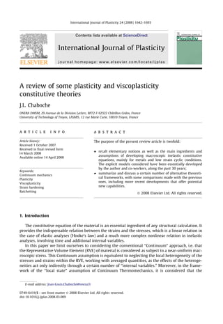
  • 6. For certain materials, an effect of saturation of the rate effect can be felt in the high rate regime. Fig. 3 shows the example of 316L stainless steel at 550 °C. The intermediate velocity range, where the rela- tion between log10rv and log10 _ ep appears to be approximately linear with a slope of n ¼ 24, extends to low rates by a rapid drop in the stress (due to static recovery phenomena that will be studied further on) and by a stress saturation at high velocities between 103 and 101 s1 . Various expressions may be proposed to express such a saturation effect in the viscosity function. They are studied and com- pared in Section 5.7. 3.3. Isotropic hardening equations When we consider the expression for the norm of the strain rate (15), by replacing f with (9), we find: _ p ¼ k r X k R k D * +n ð17Þ We find three possibilities for introducing a hardening of the isotropic type: (i) through the variable R, by an increase in the size of the elasticity domain, (ii) by increase of the drag stress D, (iii) by coupling with the evolution law of the kinematic hardening variable X . In the first two cases, the only ones considered here, we just have to define the one-to-one relation- ship between R (or D) and the state variable of the isotropic hardening, which is the accumulated plas- tic strain p (or possibly the accumulated plastic work Wp). R ¼ RðpÞ D ¼ DðpÞ ð18Þ One possibility among others is to let the two evolutions be ‘‘proportional.” We can then define only the function RðpÞ and deduce from it DðpÞ ¼ K þ fRðpÞ ð19Þ where K is the initial value of the drag stress and f is a weighting parameter. One special case, corre- sponding to the Perzyna (1964) approach, is the one obtained with K ¼ k and f ¼ 1. By decomposition of the equivalent von Mises stress (in the case without kinematic hardening, X ¼ 0), we can note the different roles of the two types of isotropic hardening req ¼ k þ RðpÞ þ rvð_ p; pÞ ¼ k þ RðpÞ þ DðpÞ_ p1=n ð20Þ Fig. 3. Overstress vs plastic strain rate on 316 L Stainless Steel at 600 °C, and its interpretation with the double slope and exponential functions. J.L. Chaboche / International Journal of Plasticity 24 (2008) 1642–1693 1647
  • 7. In the first case, with R, the elastic domain will be increased in the same way whatever the strain rate. In the second, the increase in D will cause an increase in req that will be greater with greater strain rate. The simplest and most used form of viscoplasticity equation with isotropic hardening is the one that is deduced from the combination of the secondary creep law (Norton’s law with a power function between the secondary creep rate and the applied stress) and the primary creep law (power relation between strain and time). Such approaches may be found in Rabotnov (1969), Lemaître (1971). It is equivalent to neglecting, in (17) any elasticity domain ðk ¼ 0Þ, the corresponding harden- ing RðpÞ, and adopting a power function for the drag stress D. This would be expressed: req ¼ Kp1=m _ p1=n ð21Þ This multiplicative form of the work hardening is very practical to determine (Lemaître, 1971) and yields good results in a rather large domain, at least for quasi-proportional monotonic loadings. 3.4. Kinematic hardening equations As kinematic type of hardening is a nearly general occurrence, at least in the range of moderate strains, the corresponding models will have to be used when we want to correctly express either non-proportional monotonic loadings (variation of the loading direction, thermomechanical loadings, etc.), or cyclic loadings. The most widespread kinematic hardening models are indicated here in increasing order of com- plexity. A few more advanced models for expressing special effects can be found in Sections 7 and 8. For the time being, we are discussing only strain hardening, while the time recovery effects are con- sidered in Section 3.7. The simplest model is Prager’s linear kinematic hardening (Prager, 1949), in which the evolution of the kinematic variable X (called back-stress) is collinear with the evolution of the plastic strain. Thus _ X ¼ 2 3 C _ e p and X ¼ 2 3 Ce p ð22Þ The linearity associated with the stress–strain response (Fig. 2-b) is rarely observed (except perhaps in the regime of significant strains). A better description is given by the model proposed initially by Arm- strong and Frederick (1966)1 introducing a recall term, called dynamic recovery: _ X ¼ 2 3 C _ e p cX _ p ð23Þ The recall term is collinear with X (as in the general Eq. (13)) and is proportional to the norm of the plastic strain rate. The evolution of X , instead of being linear, is then exponential for a monotonic uni- axial loading, with a saturation for a value C=c. That is, the integration of (23) with respect to ep, for a uniaxial loading, yields: X ¼ m C c þ Xo m C c expðmcðep epo ÞÞ ð24Þ in which m ¼ 1 gives the flow direction and where X0 and ep0 are the values of X and ep at the begin- ning of the loading branch considered. For strain-controlled cyclic loading, it is shown that the stabilization occurs when Xmax þ Xmin ¼ 0: DX 2 ¼ jXoj ¼ C c tanh c Dep 2 ð25Þ Fig. 4 gives the example of a few materials, treated in the rate-independent case, in which the cyclic curve is described with (25) and Dr 2 ¼ DX 2 þ k. 1 Interesting to note: this work was never published, only available as a Technical Report from CEGB (Central Electricity Generating Board). By using this rule in the context of unified viscoplasticity and generalising it continuously, the author contributed to the knowledge and citation of this report. In 2007, it has been published in ‘‘Materials at High Temperature”, accompanied with a Preface retracing this story (Frederick and Armstrong, 2007). 1648 J.L. Chaboche / International Journal of Plasticity 24 (2008) 1642–1693
  • 8. A better approximation, given in Chaboche et al. (1979), Chaboche and Rousselier (1983), consists in adding several models such as (23), with significantly different recall constants ci (factors from 5 to 20 between each of them): X ¼ X M i¼1 X i _ X i ¼ 2 3 Ci _ e p ciX i _ p ð26Þ allowing the expression of a more extensive strain domain and a better description of the soft transi- tion between elasticity and the onset of plastic flow. Fig. 4 shows, for 35NCD16 hard steel, the signif- icant improvement in the case where only two variables are superposed, one being linear, with c2 ¼ 0. Let us note here that the number of parameters introduced by such a superposition of back-stresses (set of fci; Cig) should not be considered as material parameters but as a series decomposition of a sim- pler expression of the tensile curve (or cyclic curve), for instance by a power law. This has been proved later by Watanabe and Atluri (1986), based on the endochronic theory of Valanis (1980). Other more complex combinations can be used (Cailletaud and Saï, 1995) instead of (26), but they do not allow analytical closed form solutions in uniaxial loading. In Section 7 we will also indicate var- ious modifications of the basic AF rule used above, especially in order to improve plastic ratchetting predictions by the constitutive models. 3.5. Cyclic hardening–softening In the framework of kinematic hardening models, isotropic hardening is generally used to express the cyclic evolution of the material’s mechanical strength with respect to the plastic flow. This cyclic hardening phenomenon (increase of strength) or cyclic softening (decrease) is relatively slow, typi- cally taking between ten and a thousand cycles of ep ¼ 0:2%, for example, before stabilizing. We can control the dimension of the elasticity domain with a law of the type: _ R ¼ bðQ RÞ_ p ð27Þ which is the direct transposition of (23) to isotropic hardening, with b and Q being two coefficients depending on the material and on the temperature (b will be included between 50 and 0.5 to ensure the typical saturation mentioned above in 10 and 1000 cycles, respectively). The integration of (27) leads to an expression RðpÞ ¼ Qð1 expðbpÞÞ that can also be used in the context of monotonic load- ings (but a much higher value is then needed for b). Fig. 4. Cyclic curves on various materials and their interpretation by the AF rule or the multikinematic model. J.L. Chaboche / International Journal of Plasticity 24 (2008) 1642–1693 1649
  • 9. Fig. 5, reproduced from Goodall et al. (1980), shows the example of 316 Stainless Steel, using a nor- malised plot of the maximum stress evolution as a function of the accumulated plastic strain: rM rM0 rMS rM0 ¼ 1 expðbpÞ ð28Þ where rM is the current maximum stress, rM0 and rMS being the corresponding initial (1st cycle) and stabilised values. The figure shows the validity of the choice (27) because the normalised experimental responses are approximately independent on the plastic strain range, as the model assumes. Let us note that, in the case of cyclic softening, we can set Q 0, so that the stabilised yield surface size k þ Q will be lower than the initial one (R is assumed to be the change in the size, usually with Rð0Þ ¼ 0. Also note that the drag stress D can be used in place of the yield stress R, or the two can be combined, or a coupling can be introduced between the kinematic hardening and isotropic harden- ing (Marquis, 1979) with a function /ðpÞ to be defined _ X i ¼ 2 3 Ci _ e p ci/ðpÞX i _ p ð29Þ Fig. 6 illustrates the case of 316 SS with the function / defined as / ¼ /1 þ ð1 /1Þ expðbpÞ. It shows a slight dependency on the plastic strain range but not in contradiction with experimental results. Another possible choice of /ðpÞ consists in using the variable R with a dependency deduced from an endochronic type theory (Valanis, 1980; Watanabe and Atluri, 1986): /ðpÞ ¼ 1=ð1 þ xRðpÞÞ ð30Þ Remark. Let us recall here, without more details, that endochronic theory of plasticity developed by Valanis (1980) is one based on the hereditary form of thermodynamics of irreversible processes, though the present formulations are developed in the context of thermodynamics with internal variables (Germain, 1973). See a few more details in Section 4.1.2. Such hereditary theories, like in viscoelasticity, uses the complete history of observable variables (strain and temperature), without using the notion of internal variables. This is done by integral equation to relate stress and strain tensors histories, which kernel contains most phenomenological information. This is the case for instance with the theory developed in France by Guélin and co-workers (Guélin and Stutz, 1977; Boisserie et al., 1983). It is interesting to underline here the following fact: as demonstrated first by Watanabe and Atluri (1986), when using the Valanis theory, for computational purpose, a decomposition of the kernel into Fig. 5. Modelling of isotropic hardening with the yield stress evolution for 316 Stainless Steel at room temperature (from Goodall et al., 1980). 1650 J.L. Chaboche / International Journal of Plasticity 24 (2008) 1642–1693
  • 10. a series of decaying exponentials, the model recovers kinematic hardening/isotropic hardening separation, and, surprisingly, the back-stress obeys exactly to the multikinematic rule (26) (a superposition of as many AF type back-stresses than terms in the series). The only difference is that the accumulated plastic strain dependency of the yield stress automatically appears in the forms (29), (30) above of coupling effect in the back-stress evolution equations. 3.6. Strain range memorisation and out-of-phase effects Under cyclic conditions, for some polycrystalline materials, like OFHC copper or Stainless Steels, in fact materials with a low stacking fault energy, special cyclic hardening effects can be observed, which we classify here as (1) Plastic strain range memorisation effects: after applying a large cyclic strain range, the subsequent materials behaviour has been hardened. For lower strain ranges the stabilised cyclic strength is higher than under normal cyclic conditions without a prior hardening at a larger strain range. On the other hand, as shown on Fig. 7, for the increasing level cyclic test on 316 Stainless Steel, after stabilisation of cyclic hardening at a low strain range, a subsequent cyclic hardening is still possible when applying a larger strain range (Chaboche et al., 1979). Such a behaviour is clearly not reproducible by the isotropic hardening law (27), in which R saturates only once to a fixed value Q. For such materials the cyclic curve (relation between stress range and plastic strain range under stabilised conditions) is no more a unique relationship and clearly depends on the previous loading histories. (2) Out-of-phase effects: For materials that harden cyclically, if non-proportional multiaxial loadings are applied (under strain control for instance), the cyclic hardening effect can be drastically increased and the stabilised cyclic response (in terms of von Mises invariants of the stress amplitude and plastic strain amplitude) is much more resistant than under equivalent propor- tional conditions. This fact was observed first time by Lamba and Sidebottom (1978) for OFHC copper, and has been reproduced later on several other materials, especially Stainless Steels (Kanazawa et al., 1979; Cailletaud et al., 1984; Tanaka et al., 1985; McDowell, 1985; Benallal and Marquis, 1987). Such an effect can be understood from crystal plasticity and dislocation behaviour: under a non-proportional multiaxial cyclic loading, many more slip systems are acti- vated, which increases the number of obstacles for subsequent slip to take place. Fig. 6. Modelling of isotropic hardening with the Marquis modification of the dynamic recovery term, for 316 Stainless Steel at room temperature. J.L. Chaboche / International Journal of Plasticity 24 (2008) 1642–1693 1651
  • 11. We will not be able to give detailed models of such situations. Let us only summarises the existing possibilities, in terms of macroscopic phenomenological models, as follows: (1) For the plastic strain range memorisation, a simple way was proposed in Chaboche et al. (1979) that introduces a new internal state variable, called q. Its evolution rule, not given here, mem- orises progressively the current plastic strain range (under any multiaxial conditions) provided it is larger than previously encountered ones. Such a memory variable is taken into account in the plastic flow rule by its influence on the asymptotic value of isotropic hardening Q, which now becomes a varying quantity QðqÞ. The initially proposed rule has been generalised by Ohno (1982), Ohno and Kachi (1986), as the cyclic non-hardening range. Moreover, in Nouailhas et al. (1983a), a more sophisticated model, in which some part of the memory was slowly evanescent, was used in order to describe both monotonic and cyclic hardening of (annealed) 316 SS, but also, with the same model parameters, many different cold worked initial conditions of the same stainless steel. (2) For the description of out-of-phase effects, still using macroscopic models, several attempts have been made in the eighties (McDowell, 1983; Benallal et al., 1985; Krempl et al., 1986; Tanaka et al., 1987). One of the simplest and best rule was proposed by Benallal et al. (1989), using a scalar parameter A based on the current tensorial product of the back-stress and the back-stress rate. The effect interacts with the flow rule by increasing the limit of isotropic hard- ening QðAÞ in a way similar to the above method of strain range memorisation. Such a model was working quite well and, to some extent, was able to describe also the strain range memory: for a proportional cyclic loading A is more or less related with the current amplitude of the back- stress. Another interesting approach was given by Tanaka et al. (1987), introducing a structural tensor (or polarisation tensor) as well as a non-proportionality parameter. A recent presentation of this approach was given by Tanaka (2001). Among the additional possibilities, we can indicate the model developed by Teodosiu and co-work- ers (Hu et al., 1992; Teodosiu and Hu, 1995), in which the limits of the kinematic hardening variables Fig. 7. Experimental response for the 5 levels increasing strain-controlled loading on 316 Stainless Steel at room temperature (from Chaboche et al., 1979). 1652 J.L. Chaboche / International Journal of Plasticity 24 (2008) 1642–1693
  • 12. and the coupling effects with isotropic work hardening are introduced specifically. This kind of kine- matic hardening model, differs from the above considered Armstrong–Frederic type, by the use of spe- cific polarisation tensors. This is a little more complex but is justified by physical considerations involving the dislocation substructures. A slightly different form of strain range memorization has been used recently by Yoshida et al. (2002), Yoshida and Uemori (2002), in order to better describe the work hardening stagnation effect appearing in finite strain reverse plasticity. Modelling of such effects is important in the context of sheet metal forming. The memorization model is written in the stress space, instead of plastic strain, and is coupled differently with the isotropic and kinematic hardening. This model also describes a mean-strain dependency. 3.7. Static recovery Hardening recovery with time, whether kinematic or isotropic, generally occurs at high tempera- ture. These thermally activated mechanisms are described macroscopically by relations such as (13). Thus, for kinematic hardening, we will use for example a power function in the recall term acting as a function of time (Chaboche, 1977a): _ X i ¼ 2 3 Ci _ e p ciX i _ p ci siðTÞ kX ik Mi 0 @ 1 A mi1 X i ð31Þ where mi; si; Mi depend on the material and temperature. In practice, we let Mi ¼ Ci=ci and the time constant si will be strongly dependent on the temperature. For the static recovery of isotropic hardening, we use any function, for example in Nouailhas et al. (1983b), Chaboche and Nouailhas (1989): _ R ¼ bðQ RÞ_ p crjR Qrjm1 ðR QrÞ ð32Þ which yields correct results for 316 L stainless steel. Fig. 8 illustrates this with cyclic relaxation test results in controlled strain ðDe ¼ 1:2%Þ, incorporating a more or less long tensile hold time. The longer the hold time, the less the maximum stabilized stress, which is the result of a reduction of the cyclic hardening effect obtained by the compromise of the relation (32), between hardening by strain (the first two terms) and recovery by time (the last term). Moreover, the relaxed stress (difference between the maximum value and the value rrel after relaxation) increases greatly, which also requires the inclusion of the static recovery of the kinematic variables with (31), the parameters of which have been identified by long-duration creep tests (Chaboche and Nouailhas, 1989). Fig. 8. Cyclic relaxation on 316 L Stainless Steel at 600 °C and its modelling by a unified viscoplastic model with strain range memorisation effect and static recovery effects. J.L. Chaboche / International Journal of Plasticity 24 (2008) 1642–1693 1653
  • 13. 3.8. Limiting rate-independent case In all of the above we have dealt with the case of viscoplasticity, with a part of the stress that is dependent on the strain rate (relations of Section 3.2). When the temperature is low enough, the vis- cosity effect can be neglected. For certain applications, even at high temperature, we may also want to use the rate-independent plasticity scheme. To do this in a relation like (15) or (20) we have two op- tions: reducing the drag stress D to a zero value – having exponent n that tends toward infinity. In the first case, it necessary follows that rv ! 0 and that the criterion f 6 0 will be automatically met. Of course, in an expression like (15), we end up with an indetermination (0/0), but this is deter- mined by a consistency condition f ¼ _ f ¼ 0 in the case of plastic flow. In the second case, we have rv ! 0 and f D 6 0. The formal treatment of rate-independent plasticity is somewhat more complex than that of viscoplasticity, as it further brings in a loading/unloading condition and additional difficul- ties when the material is of the negative hardening type (plastic softening). These aspects will not be discussed here. The monotonic or cyclic viscoplasticity equations, with the associated hardening models, simply degenerate in the rate-independent case, with no other change than the dimension of the pure elas- ticity domain (see Section 3.9). Let us mention the particular case of isotropic hardening, for which relation (20) becomes: req ¼ k þ RðpÞ ð33Þ Quite often in applications, the relation RðpÞ can be considered as defined point by point from the expression r ¼ k þ RðepÞ, equivalent in the uniaxial case. This function is then directly drawn from the experimental tensile curve. Quite often it can be likened to a power function, as in the req ¼ k þ Kp1=m ð34Þ 3.9. Determination methods The determination of unified viscoplasticity models combining isotropic hardening, kinematic hardening, recovery and viscosity effects, can be fairly strenuous work. Here, we propose a determi- nation process by close approximations that has often proved its worth. 3.9.1. Determination of hardening equations in the rate-independent scheme Suppose we have uniaxial tests in monotonic and cyclic loading, such as low-cycle fatigue tests up to the stabilized cycle, with r ep recorded. Let us also suppose that these are performed for velocities that are fairly constant ð_ e ConstÞ and relatively high (_ e ¼ 104 or 103 s1 , for example). From the cyclic curve, considering that _ ep _ e Const. at the cycle maxima, we will identify the following rela- tion, which is valid after stabilization of the cyclic hardening or softening effects: Dr 2 ¼ k þ R s þ X M i¼1 Ci ci tanh ci Dep 2 ð35Þ in which k is the sum k þ K _ p1=n assumed to be about constant. R s is the stabilized value of R but may also include the hardening effect that is present in the drag stress. ci accounts for any coupling with the isotropic work hardening (ci replaced by ci/sat). In practice, if the number of back-stresses is suf- ficient (three, for example), we will try to adjust k þ R s to get the lowest possible value. The third variable can be assumed linear and the slope of the cyclic curve in the region of the high amplitudes (2–3%) will provide the value of C3. We then complete the determination of the (rate-independent) equations with the available data in monotonic tensile loading and possible subsequent compression, with the corresponding experimen- tal curve being expressed by r ¼ k þ R ðpÞ þ X M i¼1 Ci ci ð1 expðciepÞÞ ð36Þ 1654 J.L. Chaboche / International Journal of Plasticity 24 (2008) 1642–1693
  • 14. The rapidity coefficient of the isotropic hardening, b, will be provided by the number of cycles needed to saturate the cyclic hardening or softening with a set amplitude Dep=2: A value near 2bNDep 5 is a good saturation criterion of the exponential. A more precise way is to plot the successions of normal- ized maxima ðrmaxðNÞ rmaxð0ÞÞ=ðrmaxðNsatÞ rmaxð0ÞÞ as a function of p 2NDep for a few low-cycle fatigue tests, as shown in Fig. 5 above. An iterative processing of all of this data, with a few readjust- ments, provides k ; Ci; ci; Q; b (and the function /ðpÞ). In case of strain range memorisation effects, when they are evidenced by multilevel or incremental cyclic straining, it is also during the present rate-independent step that the corresponding parameters can be determined. 3.9.2. Determination of the viscosity equation We now use the available data in the variable _ ep velocity domains between, let us say, 108 s1 and 104 s1 , to determine the viscosity equation, for example the exponent n, the constant K and the final value k of the true elasticity domain. We note the need for the following readjustment: k ! k þ K _ p 1=n ð37Þ R ðpÞ ! ð1 þ f_ p 1=n ÞRðpÞ ð38Þ between the version already determined in the rate-independent approximation (with a rate about equal to _ p ) and the complete version, considering the choice (19) for the isotropic hardening associ- ated with the drag variation. If we have monotonic or cyclic relaxation tests, the determination of n and K will be greatly facilitated, with the possible use of a graphic determination method (see Lemaî- tre and Chaboche, 1985). A few iterations are needed to reach a satisfactory solution (in all these analyses, we use the parameters determined in step 1). 3.9.3. Determination of static recovery effects We use the data available in a regime of very low velocities ð_ ep 108 s1 Þ, in long-duration creep or relaxation tests. As Fig. 3 illustrates for 316L, the effect of the recovery mechanism appears directly visible by the great reduction of the stress supported for a given strain rate. By successive approxima- tions, all the other parameters remaining fixed, it is relatively easy to get the static recovery param- eters of the models considered ðmi; si; Qr; mr; crÞ. If we have specific recovery test, these effects and the corresponding parameters can be measured more directly. Such tests are, for example, a normal cycling up to stabilization, then a partial discharge and a hold, at temperature, of significant duration (100 h, for example), then cycling again. The recov- ery should be carried out at a sufficiently low, but non-zero, strain or stress level, chosen such that the partial restoration of the plastic strain cannot occur. Comparison and identification of the responses before and after recovery then provides the parameter values sought very directly. 3.10. Generalisation to initially anisotropic materials Such a set of constitutive equations is quite easy to generalise in the context of an initially aniso- tropic material. In case of orthotropy, we may use Hill’s criterion in place of von Mises and fourth rank tensors in the evolution equations for the back-stresses. Such generalisations were used for example by Nouailhas (1990), in the context of a single crystal constitutive modelling. In that case Hill’s criterion is not sufficient and should incorporate higher order invariants, as shown in Culié and Nouailhas (1993). Several unified constitutive models have also been developed in order to include such possibilities of initial anisotropy, for instance in VBO theory (Lee and Krempl, 1991) and in Delobelle’s model (Delobelle et al., 1995), among those approaches discussed in Section 5. 4. Temperature effects and microstructural evolutions 4.1. Influence of temperature under stable conditions In the previous sections, the constitutive equations were presented in an isothermal context. Influ- ence of temperature was only underlined for those phenomena, like viscoplasticity or static recovery, J.L. Chaboche / International Journal of Plasticity 24 (2008) 1642–1693 1655
  • 15. that are thermally activated. In fact, there are many parameters in the constitutive equations that may be considered as depending on temperature. 4.1.1. Parametric dependency on temperature By stable conditions we indicate the normal ones, without microstructural evolutions, at least without changes in the mechanical properties that could be induced, at a given temperature, by fac- tors related independently to the history of temperature (or to both T and _ T). In those cases, the influence of temperature on the material parameters in the constitutive equa- tions may be introduced simply by interpolation techniques, linear, parabolic, spline functions, etc. Each parameter can be temperature dependant, like with parabolic expressions: CðTÞ ¼ aiðT TiÞ2 þ biðT TiÞ þ ci for Ti T Tiþ1 ð39Þ The choice of interpolating functions should expect the parameters values determined independently at the various temperatures where experimental data were available. Most often, doing so, there is a need for some iterations. At this stage, it is necessary to check on one or two normalising quantities, like 0.2% proof stress, stress to 1% creep in 100 h, or others, the correct fitness and monotonicity of the quantity even at intermediate temperatures where full experimental data were not available for a complete determi- nation of the material constitutive parameters. In some case (Cailletaud et al., 2000), with modern optimisation capabilities, the identification pro- cedure could be done all temperatures together, indentifying with all test together the chosen material functions of temperature. However, such an automatic process should be applied carefully, depending on the availability of sufficient experimental informations. Let us note the interest for some normalisation of parameters. This point can be exemplified with the simple power law for the viscosity function, which can be written simply as _ p ¼ rv DðTÞ nðTÞ or _ p ¼ _ e rv D ðTÞ nðTÞ ð40Þ The temperature dependency in exponent n is the cause of rapid variations in the drag stress DðTÞ when using the first expression (in that case DðTÞ is the viscous stress value when _ p ¼ 1). Due to the usual rate domain at which the constitutive equations are used, most often below 103 s1 , it may be much better to use the second expression, choosing arbitrarily the normalisation parameter _ e ¼ 104 s1 for instance, giving to D ðTÞ the character of a normalised drag stress for this typical strain rate. Assuming the exponent as given, we have the following obvious relation: D ðTÞ ¼ DðTÞð_ e Þ1=nðTÞ ð41Þ A different, but not incompatible, way of defining the viscosity function is given by the Zener–Hollo- mon type formulation (Zener and Hollomon, 1944), which combines the effect of the temperature and the effect of the strain rate into a single ‘‘master curve.” This approach consists in saying: _ p ¼ hðTÞZ rv DroðTÞ ð42Þ where Z is a unique monotonic function and where hðTÞ and roðTÞ are two functions of the temperature to be defined. The advantage of this formulation, illustrated in Fig. 9 reproduced from Freed and Walker (1993), is that it avoids the strong nonlinearity of a power function in which the exponent is strongly dependent on the temperature. As the function Z is defined on a large number of decades in strain rate (23, for example), the role of the function hðTÞ is then to make the useful rate domain ‘‘slide” by nor- malization (in practice limited to 6–8 decades in strain rate). The equivalent exponent (the slope of the function Z in the bi-logarithmic diagram) thus goes from a very low value in a certain region of the curve (low values of _ p=hðTÞ) to a very high value in the opposite region (high values of _ p=hðTÞ). 4.1.2. Discussion on the temperature rate term in the back-stress evolution equation The need for such an additional term, proportional to the temperature rate in the evolution equation for the back-stress, was already considered by Prager (1949) in the context of linear kinematic 1656 J.L. Chaboche / International Journal of Plasticity 24 (2008) 1642–1693
  • 16. hardening. Introduced also by the author in the unified viscoplastic constitutive equations using the nonlinear Armstrong–Frederick format (Chaboche, 1977b), it was a subject of discussion all along the past twenty years, for instance by Walker (1981), Moreno and Jordan (1986), Hartmann (1990), Ohno et al. (1989), Ohno (1990), Lee and Krempl (1991). For kinematic hardening this rate term, con- sidered as necessary for obtaining stable conditions, is as follows (only one back-stress is considered here): _ X ¼ 2 3 CðTÞ_ e p cX _ p þ 1 CðTÞ oC oT X _ T ð43Þ Compare to Eq. (23) to see the role of the temperature rate term, directly induced by the variation of ‘‘C” parameter, more or less the hardening modulus in the model. There are several arguments for such an additional term. The discussion is made here for the kinematic hardening but some arguments are valid for other hardening rules: (1) On the physical level the true state is defined by the dislocation arrangements, and the plastic strain incompatibilities (from grain to grain). Those quantities are all directly associated with the plastic strain. For the same microplasticity state, if we rapidly change the temperature, we do change Young’s modulus, which immediately changes the internal stress fields associated with the various strain incompatibilities. This is the reason why, in Miller’s unified model (see Section 5.1), the back-stress is normalised by Young’s modulus; (2) From the thermodynamic point of view, and consistently with the first remark, we usually con- sider a state potential (Helmholz free energy), that is depending on ‘‘strain like” hardening state variables: w ¼ weðe e ; TÞ þ wpða ; TÞ ð44Þ from which Hooke’s law (2) derives, by r ¼ ow oe e ð45Þ The truly independent state variable is then a ‘‘back strain” tensor a . If the part wp of the free energy (the energy stored in the material by kinematic hardening) is expressed as quadratic in this back strain tensor: Fig. 9. Stationary creep behaviour on Aluminium and Copper and its interpretation by a Zener-Hollomon function (from Freed and Walker, 1993). J.L. Chaboche / International Journal of Plasticity 24 (2008) 1642–1693 1657
  • 17. wpða ; TÞ ¼ 1 3 CðTÞ a : a ð46Þ we obtain the corresponding back-stress (the thermodynamic associated force) as X ¼ ow o a ¼ 2 3 CðTÞ a ð47Þ If considering a as the true independent state variable, we obtain _ X ¼ 2 3 CðTÞ _ a þ 2 3 oC oT a _ T ¼ ð _ X Þ_ T¼0 þ 1 CðTÞ oC oT X _ T ð48Þ where ð _ X Þ_ T¼0 is the rate expression for the back-stress under constant temperature conditions. (3) From the phenomenological point of view, we know that a great temperature dependency is possible for the 0.2% proof stress, so that, for example, the proof stress at low temperature T1 may be higher than the rupture stress at a high temperature T2. If we imagine now a 0.2% mono- tonic tensile plastic strain at T ¼ T1, then a rapid unloading and a rapid temperature change to T ¼ T2 (without any new plastic flow), upon reloading it is impossible to accept that the plastic flow will not begin before r0:2ðT1Þ. Clearly the correct behaviour will be to begin plastic flow for a stress around r0:2ðT2Þ. Such experimental evidences were for example given by Chan et al. (1990), when doing tensile tests interrupted by rapid temperature changes. (4) The last argument is the fact that, in the absence of this temperature rate term, and with a linear or nearly linear kinematic hardening, the hysteresis loops may shift unreasonably in stress (Wang and Ohno, 1991). A simple exercise may show such a situation (Chaboche, 1993), not reproduced here in detail. Let us consider a reversed strain cycle with temperature changes tak- ing place at the maximum mechanical strain (from low to high temperature) and at the mini- mum strain (from high to low temperature). Due to higher hardening slope CðTÞ at a low temperature, there will be, cycle-by-cycle, an unlimited increase of the maximum stress (if lin- ear kinematic hardening is used in the model). 4.2. Metallurgical instabilities and aging effects In the above, we have considered only ‘‘stable materials” for which microstructural transforma- tions are negligible or mechanically unperceivable. The effect of the temperature is in the constitutive equations, but in one-to-one fashion, for example through a dependency of the ‘‘material” parameters as a function of the temperature. Under certain temperature conditions, on the other hand, metallur- gical changes may occur, like phase changes, dissolution, precipitations, coarsening of precipitates, etc., that significantly modify the mechanical properties. The generic terms aging covers all of the ‘‘unstable” situations, of which there are: dynamic aging, due to the ‘‘dragging” of the dislocations by the atoms in solution, leads to an inverse relation in velocity (the viscosity exponent that would be negative in a certain strain rate regime). This non-monotonicity of the relation between rv and _ p is a source of instabilities (succession of localized bands) associated with the ‘‘Portevin-Le Chatelier” effect. To globally model such phenomena Miller (1987a) is using a strain rate dependency (or plastic strain rate) of the drag stress in the viscosity function. It leads to an implicit, non-unique, depen- dency of the viscous stress on the strain rate. Section 5.1 gives more details on this approach. Other solutions are possible, but we should not forget that modelling those situations in the framework of classical continuum mechanics becomes debatable, due to the strain localisation phenomena taking place in the tensile specimen. static aging, a growth in material strength with time (from a mechanical response viewpoint, this is the reverse of a static recovery), that can be expressed by an equation of the type dR ¼ hðÞdt. This phenomenon will occur for example in certain aluminium alloys at ambient temperature, for which destabilisation effects (metallurgical changes) are effective at high temperature. More or less sophisticated mechanical models have been proposed for this purpose (Marquis, 1989; El Mayas, 1994). One of the difficulties in these models is to meet (in an a priori way) the 1658 J.L. Chaboche / International Journal of Plasticity 24 (2008) 1642–1693
  • 18. thermodynamic requirements of a positive dissipation. Some related modelling aspects have been discussed for example in Chaboche (1993), Chaboche (1996).The temperature dependency of some parameter for isotropic hardening, together with the memory of maximum strain range (Section 3.6) has been used by Ohno et al. (1989) to describe some temperature history effects in 304 Stainless Steel. phase changes during heat treatment or sometimes during use. In terms of models attempting to express the mechanical consequences of these phenomena, we will mention that of Cailletaud (1979), to express the dissolutions, precipitations, growths of the c0 precipitates in superalloys for turbine blades, phenomena occurring under certain temperature cycles. This model uses two addi- tional state variables, one related to the volume fraction of the precipitates, the other to their size. It is obviously impossible here to go any further in the explanation of these phenomena and of the various modelling possibilities. 5. Other unified viscoplastic constitutive equations Many unified elasto-viscoplastic constitutive theories have been developed in the literature, since the middle seventies, especially for modelling the small strain cyclic conditions. Clearly, it is not pos- sible to describe such modelling theories in complete details. We will summarise here their main properties, underlining the important differences compared to the author constitutive equations. The notations will generally follow the ones already used in the previous sections, except when men- tioned. Only the isothermal conditions will be discussed below. 5.1. Miller’s MATMOD equations This unified viscoplastic model (Miller, 1976) uses one back-stress for kinematic hardening and a drag stress for isotropic hardening. There is no yield stress in the model (the elastic domain is reduced to one point). The viscosity function is a combination of an hyperbolic sine and a power function, such as _ p ¼ hðTÞ sinh kr=E ak D 3 2 #n ð49Þ where k:k denotes the von Mises invariant. The back-stress X ¼ E a is normalised by Young’s modulus. The main specificity of this model is the drag stress evolution equation, that contains several terms, as in Schmidt and Miller (1981): D ¼ ffiffiffiffiffiffiffiffiffiffiffiffiffiffiffiffiffiffiffiffiffiffiffiffiffiffiffiffiffiffiffiffiffiffiffiffiffiffiffiffiffiffiffiffiffiffi Fsol;1 þ Fdef ð1 þ Fsol;2Þ q ð50Þ where Fdef is the classical isotropic hardening variable. Fsol;1 and Fsol;2 are factors depending on the norm of plastic strain rate (as a parameter), in order to include an explicit representation of solute drag effects and dynamic strain aging, respectively without and with interactions to deformation mecha- nisms. a and Fdef obey a hardening/dynamic recovery/static recovery format in the form of (13). The static recovery terms use also an hyperbolic sine function. In more recent versions (Miller, 1987a, 1996), there is a coupling with the back-stress by which the asymptotic value Q of isotropic hardening is enhanced as Q þ qkak2=3 . The advantage of this term is to induce a strain range dependant cyclic hardening of the material, but with an erasing memory instead of a complete memory like in the model mentioned in Section 3.6. The expressions for the whole evolution equations are not given in detail. Compared to author’s model presented in Section 3, we may point out some differences: no yield stress and corresponding hardening, but a drag stress that includes a complex coupling with the current total strain rate; the viscosity function, as well as the static recovery terms in the Fdef and a evolution equations, uses an hyperbolic sine function; J.L. Chaboche / International Journal of Plasticity 24 (2008) 1642–1693 1659
  • 19. the back-stress temperature dependency is normalised by Young’s modulus (a is in fact a ‘‘back strain”); the back-stress evolution was linear in the first versions (Miller, 1976), no dynamic recovery term but nonlinearity due to the static recovery term. More recently, in Lowe and Miller (1986), the model was using three back-stresses of the Armstrong Frederick type; another specificity of the model is to have a limited number of functions of temperature, all expressed as Arrhénius functions with different activation energies. 5.2. Bodner’s theory This unified viscoplastic constitutive theory began with the Bodner and Partom (1975) article. First versions were using only isotropic hardening, as a drag stress. The version briefly summarised here is one of the most advanced ones, taken from Bodner (1987), that uses also a ‘‘directional hardening”. The equations are presented, showing the main differences with the author constitutive model: the viscosity function combines an exponential and a power function: _ p ¼ _ p0 exp Z req 2n # _ p0 ¼ 104 ð51Þ As it will be seen in Section 5.7 such an expression gives a tendency in opposition with most other kinetic equations; the direction of the viscoplastic strain rate is given by the stress deviator, without any translation by a back-stress as in most other models: _ e p ¼ _ p 3 2 r 0 req ð52Þ the hardening effect is entirely taken as a drag effect Z, including an isotropic part K and a direc- tional one D: Z ¼ K þ D D ¼ b : u u ¼ r ðr : r Þ1=2 ð53Þ the isotropic hardening variable follows the general hardening/dynamic recovery/static recovery format (13), with _ K ¼ m1ðK1 KÞ _ Wp A1K1 K K2 K1 r1 ð54Þ the identification with (32) is quite easy except the use of the plastic power _ Wp in place of the accu- mulated plastic strain rate as the driving factor; the directional hardening variable, introduced in the middle eighties (Bodner, 1987), follows also the general format (13), with _ b ¼ m2ðD1 u b Þ _ Wp A2K1 kbk K1 r2 b kbk ð55Þ where kbk ¼ ffiffiffiffiffiffiffiffiffiffi b : b r . The main difference with (31) is the use of plastic power as a driving factor. Let us note also the direction of the driving term u given by the stress direction in place of the stress deviator. Bodner’s model has not the temperature rate term in the evolution equation for direc- tional hardening, but it was introduced by Chan et al. (1990). The most important difference among other unified constitutive models is the introduction of directional hardening without using a back-stress. It has consequences both on the hardening effect (multiplicative instead of additive in stress) and on directionality effects. The direction of viscoplastic flow is always given by the stress deviator r 0 instead of the difference r 0 X . 1660 J.L. Chaboche / International Journal of Plasticity 24 (2008) 1642–1693
  • 20. This may have a significant impact on multiaxial non-proportional loading conditions. Such a sit- uation may be illustrated by considering the out-of-phase (90°) tension–torsion loading, a circle in the equivalent stress axes ðr; s ffiffiffi 3 p Þ, and assuming no isotropic hardening. It produces also a circular re- sponse for plastic strain and total strain ðe; c= ffiffiffi 3 p Þ, visualised in the same axes after multiplying them by 3l (l = elastic shear modulus). After some transient response, Fig. 10 shows that, under such con- ditions, the stress and plastic strain response delivered by Bodner’s equations will automatically have a phase difference of 90°. This is not the case with theories using the back-stress and the direction of Fig. 10. Simulation of the stabilised out-of-phase stress controlled cycle with a model without back-stress. Strain responses are indicated, with relative positions and directions. Fig. 11. Simulation of the stabilised out-of-phase stress controlled cycle with a single AFrule. Responses in strains and back- stress are indicated, with relative positions and directions. J.L. Chaboche / International Journal of Plasticity 24 (2008) 1642–1693 1661
  • 21. plastic flow given by the difference r 0 X . Fig. 11 illustrates schematically the case with one back- stress obeying AF rule, in which we observe the phase order by r , X , 3l e , 3le p . Many experiments under out-of-phase conditions have shown that a phase difference of 90° between stress and plastic strain is not realistic at all (Benallal et al., 1989). 5.3. Robinson’s constitutive model This constitutive equation was proposed first in Robinson (1978). More recent and advanced ver- sions have been developed by Arnold and co-workers (Arnold and Saleeb, 1994; Saleeb et al., 2001). The main specificities are as follows: the model uses a back-stress, a drag stress, a yield stress and a power function for the viscoplastic flow: _ p ¼ _ p0 kr Xk2 Y2 D2 * +n ð56Þ the evolution equations for the drag stress D and the yield stress R are not specified here (Y is given below); the back-stress evolution equation uses an hardening and a static recovery terms. However there is no introduction of a dynamic recovery effect as in other models; the non-linearity of the kinematic hardening is reproduced by a power function of the back-stress invariant kXk, called G: _ X ¼ n _ e p Gm RðkXkÞ X with ð57Þ G ¼ kXk if ðr 0 X Þ : X 0 and kXk P G0 G0 if ðr 0 X Þ : X 0 or kXk G0 8 : ð58Þ where G0 is a small valued quantity. Two advantages when doing so are: the need of only one back- stress and the possibility to have an easy smooth elastic–plastic transition, due to the quasi-infinite slope when kXk ¼ 0. However, to deal with cyclic conditions, this model imposes a very special definition for the elastic domain and for the rate of hardening: Y ¼ R if r 0 : ðr 0 X Þ P 0 Max R; X : r 0X krXk if r 0 : ðr 0 X Þ 0 8 : ð59Þ The advantage mentioned above is reduced due to the additional complexity of the modification of the elastic domain. Though continuity is enforced, there is a possible non-convexity of the effective elastic domain f ¼ kr Xk Y 6 0. Another drawback is the ‘‘indifferent character” of the kinematic hardening. After a tensile plastic flow for example, and a short stress excursion in compression, the previously positive back-stress is erased (it vanishes rapidly) and the subsequent tension results in exactly the same response than the initial tensile curve (at least when isotropic hardening is not considered). This is in contradiction with most of the experimental results. Several modifications, generalisations and improvements of the original Robinson approach have been developed by Arnold and Saleeb (1994), Saleeb et al. (2001), in the context of an extended ther- modynamic framework. The introduction of a supplementary dynamic recovery term, and complex couplings between isotropic hardening (yield and drag stresses) and kinematic hardening was solving the above mentioned difficulties, but also reducing the impact of the specificities offered by (57), (58). 1662 J.L. Chaboche / International Journal of Plasticity 24 (2008) 1642–1693
  • 22. 5.4. The Walker model When compared with the constitutive equations of Section 3, Walker’s version has many common points, and only a few differences, as follows: The viscoplastic function is a power law, without a yield stress, and isotropic hardening is intro- duced in the drag stress: _ p ¼ _ p0 kr Xk DðpÞ n ð60Þ The back-stress evolution equation is taken as _ X ¼ 2 3 ðn1 þ n2Þ_ e p X X 0 2 3 n1 e p ½n3/ðpÞ_ p þ n6kXkm1 ð61Þ There is a special asymmetry in the back-stress, given by the constant tensor X 0, that may describe an initial non-recoverable asymmetry of the viscoplastic behaviour. When X 0 ¼ 0 it is easy to check (Chaboche, 1989) the equivalence with superposing one linear back-stress and one nonlinear with the AF rule: _ X 1 ¼ 2 3 n1 _ e p ð62Þ _ X 2 ¼ 2 3 n2 _ e p n3/ðpÞX 2 _ p n6kXkm1 X 2 ð63Þ The isotropic hardening is introduced in the second back-stress evolution equation, with the Mar- quis expression: /ðpÞ ¼ 1 þ n4 n3 expðn5pÞ ð64Þ Except the fact that there is only two evolving back-stresses, the main difference is related with the static recovery effect: it takes place only for the nonlinear back-stress, and its amount is given by the norm of the total back-stress. In Walker’s equations there are temperature rate terms for the two back-stresses, not indicated in (61) above. As shown in Chaboche (1989) they are exactly in conformation with the thermodynamic framework discussed in Section 4.1.2. 5.5. The VBO theory of Krempl The theory of viscoplasticity based on overstress, developed by Krempl and co-workers (Cernocky and Krempl, 1980; Yao and Krempl, 1985; Krempl et al., 1986; Ho and Krempl, 2002), has also many common features with the constitutive model of Section 3. One of the main differences is to formulate the back-stress evolution in terms of total strain rate instead of viscoplastic strain rate: The equilibrium stress is a second rank tensor, called g , more or less equivalent with the stress state projected on the current elastic domain. The overstress is the difference r g . The viscoplastic function is directly depending on its von Mises invariant rv ¼ k r g k: _ p ¼ rv E/ðrvÞ _ e p ¼ 3 2 _ p r 0 g 0 rv ð65Þ where / may have various forms, for example: /ðrvÞ ¼ k1ð1 þ rv=k2Þk3 . The growth law for the equilibrium stress is driven by the total strain rate, but the dynamic recov- ery term is proportional to the norm of the viscoplastic strain rate: J.L. Chaboche / International Journal of Plasticity 24 (2008) 1642–1693 1663
  • 23. _ g ¼ wðrvÞ_ e ðg f Þ wðrvÞ Et A _ p ð66Þ The hardening function wðrvÞ introduces rate effects in the evolution equation for the equilibrium stress, which differs from other theories and induces various possibilities. The f tensorial variable obeys a linear kinematic hardening law, where Et is the asymptotic tangent modulus: _ f ¼ Et _ e ð67Þ Parameter A may be a material constant or a function of the accumulated plastic strain, as in the Marquis model. In some applications it has also been taken as depending on the plastic strain range memory and out-of-phase index (Colak, 2004). The standard VBO model does not take into consideration the static recovery of the equilibrium stress, but this is easy to incorporate as in other theories. It is easy to show that the VBO theory reduces to the superposition of two independent kinematic variables, g ¼ f þ x , with (67) for f and _ x ¼ ðw EtÞ _ e x A _ p ! ð68Þ In Chaboche (1989) it was shown that, under multiaxial proportional conditions and the limiting case of rate-independent plasticity, the VBO theory does coincide with the theory of Section 3 with two back-stresses (one linear and one nonlinear). The difference induced by using the concept of equilib- rium stress and the total strain rate in its evolution equation will be active only for the viscoplastic case. However, as discussed for example by Freed and Walker (1990), there could have some advan- tages concerning the modelling of ratchetting effects, provided the quasi-linear evolution of g during what is usually considered as a purely elastic loading. Let us note a specific difficulty with this VBO theory for its incorporation into a standard thermo- dynamic framework. As discussed in Chaboche (1996), it will lead to an unconventional definition for the elastic strain, due to the use of a reversible term in the evolution equation of the internal state var- iable. Such discussion was also given, in other terms in Lubliner (1973), Freed et al. (1991), Malmberg (1990). Recent efforts have been made by Hall et al. (2005) to interpret the stress rate dependent term as a dissipationless contribution. 5.6. Delobelle’s approach The unified constitutive model of Delobelle was developed initially by including two back-stresses playing role successively instead of simultaneously (Delobelle, 1988), with some complicated coupling criteria. A more recent but enhanced version is summarised here, due to the works done with Robinet (1995) and Schäffler (1997). Though existing for an orthotropic material Delobelle et al. (1995), it is written here for the isotropic particular case: the viscoplastic function is given by an hyperbolic sine like in Miller’s model: _ p ¼ _ p0ðTÞ sinh rv Dðp; TÞ n ð69Þ where the viscous stress is rv ¼ kr Xk (no yield stress); the back-stress evolution is given using a secondary and a tertiary back-stresses as _ X ¼ C 2 3 YðpÞ_ e p ðX X 1Þ_ p rmðTÞ sinh kXk X0ðTÞ m X kXk ð70Þ _ X 1 ¼ C1 2 3 YðpÞ_ e p ðX 1 X 2Þ_ p ð71Þ _ X 2 ¼ C2 2 3 YðpÞ_ e p X 2 _ p ð72Þ 1664 J.L. Chaboche / International Journal of Plasticity 24 (2008) 1642–1693
  • 24. for rapid loading conditions, or when the static recovery is negligible, the 3 evolution equations of the back-stresses are equivalent to the superposition of 3 independent back-stresses, each obeying the rule (26), as shown in Chaboche (1986); the common asymptotic value for the back-stresses YðpÞ is a given function of the accumulated plastic strain, like for example: YðpÞ ¼ Ysat þ ðY0 YsatÞ expðbpÞ. For saturation under a rapid plas- tic straining, we have: kX2k ! Y, kX1k ! 2Y, kXk ! 3Y; the drag stress Dðp; TÞ is also a given function of temperature and accumulated plastic strain; the static recovery appears only on the kinematic hardening. It is implemented directly on the main back-stress evolution equation, with an hyperbolic sine dependency, like in Miller’s approach. As in Walker’s model, it plays role as a function of the norm of the total back-stress. Concerning further modifications of static recovery of the back-stresses, we could also mention more recent ones by Yaguchi et al. (2002) and Zhan and Tong (2006). In this model there are two back-stresses. The first one obeys the classical Armstrong–Frederick expression (23), without static recovery in it. The second one introduces an additional tensorial variable Y , as _ X 2 ¼ 2 3 C2 _ e p c2ðX 2 Y Þ_ p ð73Þ _ Y ¼ a Ysat X 2 kX 2k þ Y 2 4 3 5kX 2km ð74Þ Such a modification was shown to greatly improve the modelling of relaxation, under monotonic and cyclic conditions, for new nickel-based superalloys (Zhan and Tong, 2006). 5.7. Comparison of the viscosity functions In any unified viscoplastic constitutive equation, there is a function to describe the relation be- tween the stress, or viscous stress, or overstress, and the norm of the viscoplastic strain rate. The ref- erence function is often the power law (Norton’s equation for creep) but, very often the observed exponent is varying with the stress (or strain rate) domain. In many experimental results there is the appearance of a saturation effect of the viscosity for high rates, which justify the use of an hyper- bolic sine function for instance. In the present section, we systematically compare the viscosity functions (or kinetic equations) used in the various constitutive models considered in the present Section 5. We consider also two specific expressions used in applications of Onera constitutive model, which general framework has been presented in Section 3 _ p ¼ rv D n exp a rv D nþ1 ð75Þ _ p ¼ rv D n 1 þ rv q a ð76Þ In all these expressions, the exponent n is strongly dependent on the temperature, while the viscosity phenomenon is thermally activated (n becomes small at high temperatures). We also add others, like Johnson-Cook equation used in the context of dynamic plasticity, in the high rate regime, which expresses: _ p ¼ _ p0 exp 1 C krk D 1 ð77Þ A special mention can be made here for the Kocks et al. (1975) expression, also used by many others (Busso and McClintock, 1996; Cheong et al., 2005). Let us note that it generalises Johnson-Cook ones, which is recovered when choosing p ¼ q ¼ 1: _ p ¼ _ p0 exp 1 C 1 krk D p q # ð78Þ J.L. Chaboche / International Journal of Plasticity 24 (2008) 1642–1693 1665
  • 25. In all these expressions, the exponent n is strongly dependent on the temperature, while the viscosity phenomenon is thermally activated (for instance, exponent n becomes small at high temperatures). However, temperature will not be considered in what follows. For comparison purpose, all these viscosity functions are adjusted each other by the following way: when possible, using one point ðr1; _ p1Þ with reference Norton’s exponent N0, in the low rate regime (for instance _ p1 ¼ 108 s1 ), and one point ðr2; _ p2Þ in the high rate regime (for instance _ p2 ¼ 1 s1 ) in other cases (Bodner, Johnson-Cook), we adjust only at an intermediate point ðr 1; _ p 1Þ like _ p 1 ¼ 106 s1 , at which we adjust also the equivalent exponent N0. These comparisons are made for a given state of hardening. However, the viscous stress having not exactly the same role in each theory, the comparisons are showing only qualitative tendencies. Let us note that, in most viscoplastic models, the time recovery effects that may take place under low stres- ses, low strain rates (long durations), are not taken into account in the viscosity functions studied here. They are considered as playing role directly in the evolution equations of the hardening variables, with the last term in the general format (13). Therefore, the plot made in Fig. 12, in terms of the viscous stress (at a fixed hardening state), should not contain these effects, like in Fig. 3. The considered functions and the corresponding effective exponent ðN ¼ d ln _ p=d ln rÞ are indicated in Table 1, in the uniaxial format, together with the adjusted parameters, in the case N0 ¼ 20, _ p1 ¼ 108 s1 , r1 ¼ 150 MPa, _ p2 ¼ 1 s1 , r2 ¼ 300 MPa, _ p 1 ¼ 106 s1 , r 1 ¼ 190 MPa. Fig. 12 presents a log–log plot of the viscous stress (or stress) as a function of the viscoplastic strain rate. The following trends are clearly evidenced: three models perform quite similarly, having the same exponent N0 ¼ 20, in the low rate regime: the Delobelle hyperbolic sine and the two Onera versions; Fig. 12. Comparison of viscoplastic flow functions, overstress vs plastic strain rate. Norton’s exponent N ¼ 20 in the interm- ediate regime 108 _ ep 104 s1 . 1666 J.L. Chaboche / International Journal of Plasticity 24 (2008) 1642–1693
  • 26. the double slope version is interesting in the sense it limits the equivalent exponent value for high rates, which may have positive consequences at the numerical stage when using explicit time inte- gration schemes; Krempl and Miller expressions give much less saturation effect. If enforced to pass the point r2, _ p2, in the intermediate regime 105 _ p 101 s1 they do not perform as the previous ones. Another adjustment is possible, as shown on the figure, but it does not change the general tendencies; Bodner’s model leads to a totally inverse tendency, with an increasing viscosity effect (or a decreas- ing effective exponent N). It may be adjusted to the other models only in the regime 109 _ p 104 s1 . Let us recall that the generally observed trends are opposite to this model; Johnson-Cook expression, usually applied in the high rate regime (dynamic plasticity), when adjusted here for 108 _ p 101 s1 , shows a slower saturation effect (like Krempl and Miller expressions). Moreover it leads to a significant underestimation of the stress in the low rate regime compared to Norton’s like expression, which may lead to a questionable trend; Table 1 Comparison of various viscosity functions and corresponding effective exponents Model Viscoplastic strain rate _ p Equivalent exponent N Values of parameters Onera exponential ðr D Þn expðaðr D Þnþ1 Þ n þ aðn þ 1Þðr D Þnþ1 n ¼ N0; D ¼ 376:8; a ¼ 546:5 Onera double slope ðr D Þn ½1 þ r q a n þ a 1þðr=qÞa n ¼ N0; D ¼ 376:8; a ¼ 50; q ¼ 274 Krempl r Ek1 ð1 þ r k2 Þk3 1 þ k3 r k2 þr Ek1 ¼ 1:1023 ; k2 ¼ 93:3; k3 ¼ 31 Miller B½sinh r D
  • 27. 1:5 n 3 2 n r D
  • 28. 1:5 Th 1 ðr D Þ1:5 n ¼ 2 3 N0; D ¼ 311:2; B ¼ 0:017 Delobelle A sinh r D
  • 31. n n ¼ N0; D ¼ 271:8; A ¼ 0:00145 Bodner _ p0 exp Z r
  • 33. 2n n ¼ 0:395; Z ¼ 11095; _ p0 ¼ 105 Johnson-Cook _ p0 exp½1 C r D 1
  • 34. r CD C ¼ 1=N0; D ¼ 190:; _ p0 ¼ 106 Kocks _ p1 exp½ 1 C h1 ðr D Þp iq pq C r D
  • 35. p h1 ðr D Þp iq1 p ¼ 0:1; q ¼ 0:44; D ¼ 328:5; C ¼ 0:0107; _ p1 ¼ 105 Fig. 13. Effective exponent of the power law as a function of overstress for various viscoplastic flow functions. J.L. Chaboche / International Journal of Plasticity 24 (2008) 1642–1693 1667
  • 36. the Kocks expression having more degrees of freedom (exponents p and q) allows a better represen- tation than Johnson-Cook. It leads to a saturation effect in the high rate regime (complete saturation when r ! D), but less pronounced than Onera exponential or Delobelle’s hyperbolic sine. More- over, in the low rate regime, this choice leads to lower stresses than in the power law. Though it needs to modify consequently the recovery effects (compared to the previous models), it could be a good alternative. Fig. 13 shows the evolution with the strain rate of the effective exponent N for all the models. It confirms the trends observed above: the Delobelle and Onera models have a constant exponent for low rates, then increasing, which leads to saturation of the viscosity effect. Krempl, Miller and John- son-Cook shows a continuously increasing exponent, but no saturation effect; Kocks expression is somewhat intermediary. Bodner’s model gives a decreasing exponent, contrary to all other models. The same exercise, repeated for lower reference exponents, N0 ¼ 10, N0 ¼ 5, N0 ¼ 3, shows exactly the same qualitative trends. However, the domains in which every models can be adjusted each other is further reduced: 108 to 104 for N0 ¼ 10 and 106 to 104 for N0 ¼ 3. 6. Other types of modelling 6.1. Plasticity–creep partition This is the oldest way of describing plasticity and creep phenomena simultaneously, by adding two independent inelastic strains. Eq. (1) is then replaced by e ¼ e e þ e p þ e c ð79Þ Let us note immediately that the plastic strain e p of the previous Sections included both the plasticity and creep effects in unified fashion. Here, on the other hand, we consider that they are separate and generally independent. The variations of the two inelastic strains will then be described: by rate-independent plasticity theory for e p with a normality rule such as (4), and in association with the hardening equations that are appropriate for the type of application considered, isotropic hardening for applications under quasi-monotonic loading, kinematic hardening or a combination of the two for applications under cyclic loading or when non-proportional multi-axial effects may arise. Without explaining, these can be written formally: _ ap j ¼ h p j _ ep rp j ðap j ; . . .Þap j _ ep ð80Þ The advantage of decoupling between plasticity and creep is that it makes it easy to determine material’s parameters either from the monotonic tensile curve or from the cyclic curve (step 1 in Section 3.9). by a creep type of law for e c , incorporating primary creep and secondary creep, in an integrated form such as ec eqðreq; tÞ ¼ A1ðreqÞt1=p þ A2ðreqÞt ð81Þ in which req is the von Mises equivalent stress, as defined from (5) and (8), and ec eq is the equivalent creep strain, defined in the same way as p in (11). In place of (81) a differential form is more correct, because it brings in the strain hardening: _ ec eq ¼ gcðreq; ec eqÞ ð82Þ for which we can also take up an hardening equation of the multiplicative type such as (21), by replacing p by ec eq. Here it must be underlined that such a creep equation with isotropic strain hard- ening cannot correctly describe cyclic creep conditions, that show evidence of successive primary creep periods after each reversal. It is also possible to adopt a form such as (13), with additional hardening variables (combining isotropic and kinematic hardening): _ ac j ¼ h c j _ ec rc j ðac j ; . . .Þac j _ ec ð83Þ 1668 J.L. Chaboche / International Journal of Plasticity 24 (2008) 1642–1693
  • 37. This form of evolution law combines strain hardening and static recovery (effect of time, important in long term creep). Examples of such modellings may be found in Murakami and Ohno (1982). Here again, whatever the form of hardening equation chosen, the decoupling with the plasticity allows very easy determination either from pure creep tests or from relaxation tests. This method by partition of the inelastic strain was used routinely up until the experimental obser- vation, reported on numerous occasions, of an obvious coupling between plastic strain and creep strain, by way of the associated hardening effects. An example of experimental observations can be found in Ikegami and Niitsu (1985), among many others. Fig. 14 schematically shows the type of observation made on a quick tensile test, interrupted by a long-duration period of creep (constant stress). Clearly, there is a nearly immediate forgetting of the creep period and the experimental evi- dence that hardening is correlated with the sum ep þ ec, and not defined independently with ep or ec, which assumption should have given the horizontally translated curve on the figure. On the other hand, unified viscoplastic constitutive equations take into account the hardening in- duced by creep strain on the subsequent tensile loading, approaching better the experimental obser- vation. However, this may be quantitatively insufficient, provided strain hardening develops less significantly in creep, especially in steady-state creep, due to the effect of time recovery. This type of observation, and many others going in the same direction, have led to the development of more sophisticated non-unified approaches but with coupled hardening (Kawai and Ohashi, 1987; Contesti and Cailletaud, 1989) by writing, for example: _ ap j ¼ h p j _ ep þ h pc j _ ec rp j ðap j ; . . .Þap j ð84Þ _ ac j ¼ h cp j _ ep þ h c j _ ec rc j ðac j ; . . .Þac j ð85Þ with all sorts of possible variations. These approaches are followed relatively little, because there are determination complications or difficulties analogous to those of unified theories. 6.2. Multiple mechanisms – multiple criteria 6.2.1. A general formulation The unified viscoplastic constitutive equations consider only one inelastic mechanism, that in- cludes both plastic and viscoplastic (or creep) effects. Most of the rate-independent plasticity frame- works (limit case of the unified viscoplastic ones or others like in Section 7 and 8) are also considering a unique plastic strain variable. σ ε p c p ε ε ε + 0 tension at constant strain rate tension – creep – tension creep independent creep plasticity Fig. 14. Schematic results of the tension–creep–tension test and comparison with the test at constant strain rate. J.L. Chaboche / International Journal of Plasticity 24 (2008) 1642–1693 1669
  • 38. However, there are other approaches possible, like in slip plasticity (Mandel, 1965; Hill, 1966; Rice, 1970). A quite general presentation, used in Besson et al. (2001), can be given as follows. In viscoplasticity, we assume a collection of potentials Xs , s ¼ 1; S, dependent on r and hardening variables AJ through a yield function fs ðr ; AJÞ. The plastic strain rate is a summation of the associated mechanisms: _ e p ¼ X s oXs o r ¼ X s _ vs ofs o r ð86Þ and, in the Generalized Standard Material framework (Halphen and Nguyen, 1975), the strain-like hard- ening variables evolve as _ aI ¼ X s oXs oAI ¼ X s _ vs ofs oAI ð87Þ where AI are the thermodynamic forces associated with internal state variables aI, deriving from the free energy potential by AI ¼ ow oaI ð88Þ Let us remark that AI gives generally hardening effect. Therefore, the partial derivative ofs =oAI is negative. In the rate-independent plasticity framework the _ vs are replaced by the plastic multipliers _ ks to be determined by a linear system of consistency conditions: _ fr ¼ n r : _ r þ X I ofr oAI _ AI ¼ 0 ð89Þ From (88) and (87), we get _ AI ¼ X K oAI oaK _ aK ¼ X s X K oAI oaK ofs oAK _ ks ð90Þ and (89) rewrites: _ fr ¼ n r : _ r þ X s Hrs _ ks ¼ 0 ð91Þ with Hrs ¼ X I;K ofr oAI oAI oaK ofs oAK ð92Þ Hardening manifests itself through an interaction matrix, whose components Hrs express the harden- ing induced by mechanism s on the mechanism r. Using the time derivative of Hooke’s law (2) and its projection as n r : _ r ¼ n r : L : _ e _ e p ð93Þ and using (86), we obtain the system: X s Qsr _ ks ¼ n r : L : _ e ð94Þ with Qsr ¼ n r : L : n s þ Hrs. Its solution may be written as _ ks ¼ X r Q1 sr n r : L : _ e ð95Þ and the tangent stiffness tensor writes: L t ¼ L X s X r Q1 sr L : ðn s n r Þ : L ð96Þ 1670 J.L. Chaboche / International Journal of Plasticity 24 (2008) 1642–1693
  • 39. Due to the associated plasticity framework used here (elastic domains and yield surfaces are both de- scribed by fs ) the matrices Hrs and Qrs are symmetric and the tangent stiffness tensor also has the prin- cipal symmetry. Obviously, the linear system (94) only concerns those mechanisms that are actually active. Classical crystal plasticity models (or their viscoplastic counterpart) are clearly described in this general framework (using for instance a Schmid criterion for fs ). The model used in Section 6.3 below is exactly under these lines, both at the level of single crystal viscoplasticity and for the polycrystalline formulation with a micro–macro transition rule. 6.2.2. Models with two mechanisms and two criteria (2M2C) This is an interesting particular case that can be an alternative to extend the capabilities of the macroscopic models considered in this paper. The potential is written as a sum: X ¼ X1 ðf1 Þ þ Xðf2 Þ ð97Þ with two kinematic/isotropic hardening sets and two yield criteria: fI ¼ kr XI k RI kI ð98Þ that leads to the plastic strain rate as _ e p ¼ oX1 of1 n 1 þ oX2 of2 n 2 with n I ¼ ofI o r ð99Þ The above formulation can be applied directly but it is necessary to introduce coupled kinematic hard- ening effects in the free energy, using for instance: wp ¼ 1 3 X I X J CIJa I : a J þ 1 2 X I bIQIðrI Þ2 ð100Þ Each back-strain a I obeys an Armstrong–Frederick rule like: _ a I ¼ n I 3cI 2CII X I oXI ofI ð101Þ and a similar rule for the isotropic hardening variable rI , not specified here. However their effect is coupled through the corresponding forces that play role in the potential: X I ¼ owp oa I ¼ 2 3 X J CIJa J RI ¼ owp orI ¼ bIQIrI ð102Þ The above coupled approach of a non-unified plasticity–creep theory by Contesti and Cailletaud (1989) exactly meets this framework. It suffices to chose I ¼ p and J ¼ v, and to consider (99) as a sum- mation of a plastic strain rate and a viscoplastic (or creep) strain rate: _ e in ¼ _ e p þ _ e v ¼ _ k ofp o r þ _ v ofv o r ¼ _ kn p þ _ vn v ð103Þ where _ k is an unknown plastic multiplier and _ v is a given function of the overstress fv , like a power function _ v ¼ hfv =Kin . Contesti and Cailletaud (1989) still uses AF rule for both plasticity variables a p and X p and viscoplastic ones a v and X v . However, due to the coupling effect in (102) the plastic con- sistency condition leads to a non-classical term in the plastic multiplier, like: _ k ¼ 1 Hp _ r Cvp _ a v : n p ð104Þ where Hp depends on the kinematic and isotropic hardening variables of the plastic mechanism. More elaborated forms of this approach were developed recently by Taleb et al. (2006). J.L. Chaboche / International Journal of Plasticity 24 (2008) 1642–1693 1671
  • 40. 6.2.3. Models with two mechanisms and one criterion (2M1C) It is also possible to combine several mechanisms (here only two) within only one single criterion. An example is given, proposed initially by Zarka and Casier (1979). We have two mechanisms e 1 and e 2 , and two sets of associated kinematic hardening variables, still obeying coupling relations like (102). They are combined through the single criterion: f ¼ ffiffiffiffiffiffiffiffiffiffiffiffiffiffi J2 1 þ J2 2 q R k ¼ Jeq R k ð105Þ with JI ¼ k r X I k and with a single isotropic variable. The normality rule gives: _ e p ¼ _ k of o r ¼ _ k J1n 1 þ J2n 2 Jeq ¼ _ k n ð106Þ with n I ¼ oJI=o r . In order to meet thermodynamic requirements, the first term in the evolution equation of back strains contains a factor JI=Jeq as _ a I ¼ JI Jeq n I 3cI 2CII X I _ k ð107Þ In the rate-independent framework, applying the consistency condition f ¼ _ f ¼ 0, leads to _ k ¼ 1 h n : r ð108Þ as usual, with h ¼ hX1 þ hX2 þ hR, where hX1 ¼ J1 Jeq n 1 3c1 2C11 X 1 : ðC11J1n 1 þ C12J2n 2 Þ ð109Þ hX2 ¼ J2 Jeq n 2 3c2 2C22 X 2 : ðC12J1n 1 þ C22J2n 2 Þ ð110Þ and where the isotropic hardening contribution hR is not expressed here (free choice). In such a model the plastic multiplier _ k does not correspond with the equivalent plastic strain rate as usual. An inter- esting property of such a model is that, for a non-zero determinant C11C22 C2 12, the ratchetting stops for a non-symmetric stress control, after a transient evolution, as exemplified by Fig. 15 (Besson et al., Fig. 15. Ratchetting response of the 2M1C model with a non-singular interaction matrix (from Besson et al., 2001). 1672 J.L. Chaboche / International Journal of Plasticity 24 (2008) 1642–1693
  • 41. 2001), obtained by using only linear kinematic hardening in (107), with c1 ¼ c2 ¼ 0. The fact that a linear hardening is here able to describe quite correctly the nonlinear kinematic hardening has to be underlined. Such an approach was proposed and exploited in the context of simplified inelastic analyses of shot-peening or similar processes, like in Zarka et al. (1980), or Inglebert and Frelat (1989). Some gen- eralizations are still under development. See for instance Taleb et al. (2006), Sai and Cailletaud (2007). 6.3. Micro–macro transition approaches These consist in making use of the basic crystalline plasticity equations, by writing directly in the model the various slip systems that can be activated, for the various grain orientations considered in a polycrystal RVE. Fig. 16 gives the operating scheme of such an approach, limiting itself (formally) to an imposed macroscopic stress situation r (scheme set up on a time increment), the output being the macroscopic plastic strain e p . The method uses two localization steps and two averaging steps: macro $ grain g $ slip system s Among numerous similar formulations, we follow here the one of Cailletaud (1992) and Pilvin (1994), that is rather simple to use and is, however, sufficiently precise (even if it retains a pronounced phe- nomenological character). The transition from the macro level to the (average) stress level in each grain is done by the follow- ing localization rule, of the Kröner (1961) type, but corrected with the so-called beta rule, which is va- lid for a polycrystal with grains of the same type, and with a macroscopically isotropic elasticity: r g r ¼ 2laðb g B Þ ð111Þ where l is the shear elastic modulus, a an Eshelby based adjustment parameter (near a ¼ 0:5), b g a state variable for each grain, analogous to the average plastic strain in the grain e pg , and B the corre- sponding average: r ¼ X g cgr g e p ¼ X g cg e pg B ¼ X g cgb g ð112Þ in which cg is the volume fraction of each orientation considered. Kröner’s elastic localisation rule, which is known as ‘‘too stiff” (Zaoui and Raphanel, 1993), would be equivalent to replacing b g by e pg and B by e p . The originality of Cailletaud and Pilvin’s approach is to continuously adapt this rule. Therefore it becomes ‘‘quasi-elastic” in the regime of low plastic strains, and tends toward a ‘‘tangent” type rule for higher strains, with a corresponding plastic accommodation effect. This is given by the following evolution law for b g , which is very similar to a nonlinear kinematic hardening (combined with a linear kinematic hardening): g g σ p p ε γ s s s τ γ σ ε ε . integration macroscopic constitutive equation slip constitutive equation Fig. 16. Flow chart of a polycrystal material constitutive model based on crystal viscoplasticity. J.L. Chaboche / International Journal of Plasticity 24 (2008) 1642–1693 1673
  • 42. _ b g ¼ _ e pg Dðb g de pg Þk_ e pg k ð113Þ D and d are global adjustment parameters, used to render the model similar to a self-consistent type model, from numerical finite element analyses (Cailletaud and Pilvin, 1994; Pilvin, 1997). The transition to the slip system level is done by using the resolved shear stress: ss ¼ r g : ðns ls Þ ¼ ns i rs ijl s j ð114Þ where ns and ls are, respectively, the normal to the slip plane and the slip direction. Although it is for- mally present, the index ‘‘g” of the grain is omitted for quantities associated with the slip system. In slip plasticity Schmid’s criterion writes: fs ¼ jss xs j rs k 6 0 ð115Þ In slip viscoplasticity the slip rate is given here by a power law: _ cs ¼ fs K n Signðss xs Þ ð116Þ Let us note that it represents the summation on the grain of all the slips of the same direction. Here, xs is a scalar kinematic hardening variable associated with each system and expressing the presence or development of intragranular inhomogeneities (precipitates, inclusions, walls, dislocation cells, etc.). Its evolution law obeys the nonlinear kinematic format already mentioned several times: _ xs ¼ C _ cs dx s j_ cs j ð117Þ rs is a scalar variable expressing the size variation of elastic domain for each system. It obeys a non- linear law that brings in the interactions between the various systems, a law of the type: _ rs ¼ X r hsr expðq~ cr Þ_ ~ cr ð118Þ or others of similar versions, where ~ cr is the cumulative slip on the system ‘‘r” (_ ~ cr ¼ j_ cr j). Also, hsr is the interaction matrix constructed from crystallographic informations and on studies made at lower scales (by Dislocation Dynamics for instance). It has the dimension of the number of directions of sys- tems that can be activated per grain, 12 for the octahedrals, 6 for the cubics, 18 in all in a CFC grain, etc. We note that the ‘‘material” coefficients k (initial threshold of the Schmid criterion), n, K, C, d, q may depend on the type of system to which the corresponding relation is applied (octahedral, cubic, or oth- ers for non-CFC crystals). Once the cs quantities are defined by integration over a time increment, we then have to work back to the average plastic strain of the grain: e pg ¼ X s2g cs ðns ls Þ ð119Þ and then to the macroscopic plastic strain by (112b). The scheme for a controlled macroscopic strain is the same, although it requires an iterative solution with the macroscopic elasticity equation r ¼ L : ðe e p Þ. Note: Although it is a matter of a micromechanical approach guided by the physical mechanisms, the model thus developed could just as well be called macroscopic, as it is part of the multi-criterion type approaches (Mandel, 1965) mentioned in Section 6.2. That is, the two localization rules applied remain very close and refer only to average quantities on each grain, without precise geographical localization. In effect, all of the above equations can be reduced to the use of a criterion f gs : _ e p ¼ X g;s cs fgs Kgs n fgs ¼ m gs : ðr X gs Þ ð120Þ X gs ¼ xgs m gs þ 2laðb g X g0 cg0 b g0 Þ ð121Þ where m gs ¼ ns ls , for the slip systems of the grain g. 1674 J.L. Chaboche / International Journal of Plasticity 24 (2008) 1642–1693