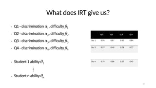
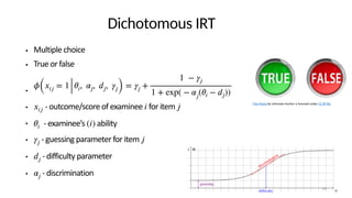
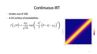
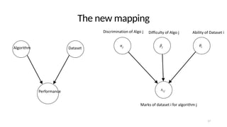
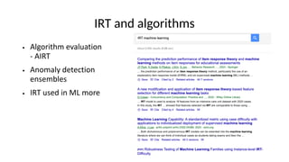
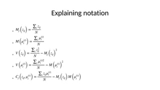
Download to read offline


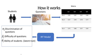


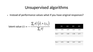
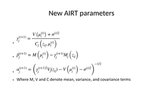
![Fitting the IRT model
• Maximising the expectation
• - discrimination parameter of algorithm
• - scaling parameter for the algorithm
• - difficulty parameter for the algorithm
• - score of the algorithm on the dataset/problem
• - prior probabilities
Eθ|Λ(t),Z [ln p (Λ|θ, Z)] = N
n
∑
j=1
(ln αj + ln γj) −
1
2
N
∑
i=1
n
∑
j=1
α2
j ((βj + γjzij − μ(t)
i )
2
+ σ(t)2
)
+ ln p (Λ) + const
αj
γj
βj
zij
Λ](https://image.slidesharecdn.com/adsnsktalknew-240106004018-0902b411/85/Explainable-insights-on-algorithm-performance-18-320.jpg)
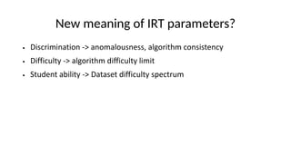

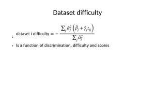


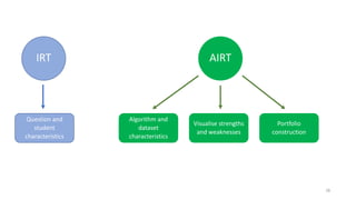


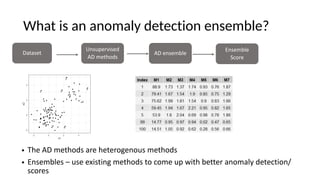
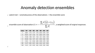
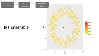


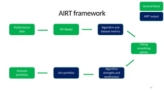


The document discusses the distinction between explanation and prediction in algorithm performance evaluation, advocating for the integration of social science methods in machine learning. It introduces Item Response Theory (IRT) as a framework for evaluating algorithms through a causal lens, allowing for a deeper understanding of algorithm strengths and weaknesses. The application of IRT in algorithm analysis can help visualize performance across various datasets and inform the selection of effective algorithm portfolios.