This document introduces a correction in the classical electromagnetic field energy density when there are discrete charges instead of a whole density of charge based in the fact that the EM field induces by a particle does not affect itself and does not contribute to the potential in the hamiltonian. A deeper analysis is done on how to deal with the radiated field energy, the reaction force and its analogy with quan Vacuum

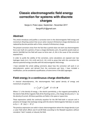
1. Classic electromagnetic field energy
correction for systems with discrete
charges
Sergio A. Prats López, September - November 2017
SergioPL81@gmail.com
Abstract
This article introduces and justifies a correction term in the electromagnetic field energy and
momentum (Poynting vector) that occurs when classical infinitesimal charge distributions are
replaced by discrete particles with a finite, instead of infinitesimal, charge.
The present correction arises from the fact that a particle does not exert any electromagnetic
force over itself, let a particle 𝒜 have a charge distribution 𝜌(𝒓), the particle would create an
electric field E(r) but this field will cause no force over 𝒜, this is the cause of the correction
exposed here.
In order to justify the validity of the correction, some calculations are exposed over two
Hydrogen levels (n=1, l=0, m=0) and (n=2, l=0, m=0) to prove that with this correction the
electron potential energy coincides with the electromagnetic field energy.
I have extended the article adding comments about how the correction will work in an
electrodynamic system and derived from the conclusions got here, I have included a
modification, can be considered a qualification, of some terms in the QED Lagrangian.
Field energy in a continuous charge distribution
In classical electrodynamics, the electromagnetic field spatial density of energy and
momentum are given by:
𝑢 = 𝜀 𝑬 + 𝜇 𝑯 𝟐
𝑺 = 𝑬 × 𝑯
Where ‘u’ is the density of energy, 𝜀 the electric permittivity, 𝜇 the magnetic permeability, E
the electric field, H the magnetic field, S the Poynting vector, 𝜌 the charge density and 𝑱 = 𝒗𝜌
the density of current. All these quantities are fields in the space or space-time.
These expressions satisfy the continuity equation for the EM field both in vacuum and in
presence of charges that exchange energy with the electric field (magnetic field does no work)
as 𝜕 𝑢 = −𝑬 · (𝒗𝜌) = −𝑬 · 𝑱
The previous expressions are valid in classic electromagnetism where the charge density is just
a scalar field which affects over E and H fields according to the Maxwell equations without
considerer “who” created, or induced, the field.

2. The field caused for a single point density of charge is order 𝑑𝑟 . Individually, it is uncappable
of making any appreciable effect on the other points or over itself, for that reason it is
irrelevant to take into account if an infinitesimal charge affects itself or not.
In a similar way, the field energy that an isolated particle would induce is irrelevant compared
with its mass energy. If we have isolated infinitesimal charges with charge density 𝜌 and mass
density m, let’s say its charge is 𝜌𝑑𝑟 and its mass m𝑑𝑟 . The energy that this isolated “charge
density” field would have, U, can be obtained as:
U =
1
2
𝜀 𝑬 𝑑𝑉 =
1
2
𝜀 𝑑𝑟
1
𝑟
2𝜋𝑟 𝑑𝑟
→
= 𝑐𝑡 ∗ 𝑑𝑟
Since 𝑑𝑟 → 0 the overall field energy is two orders of magnitude less than the mass or kinetical
energy, therefore is negligible.
So, if we had many “very small” charges “very far” from each other, and all them with the
same sign, they field energy would be negligible, if we get them closer, they will exert a
repulsive force on each other, so their kinetic energy will decrease and therefore the field
energy will increase since 𝜕 𝑢 = −𝑬 · 𝑱 = −𝜕 𝐸 , thus, field energy increases as charge
with the same sign get closer. The energy in the field is closely related to the charge’s potential
energy 𝜙, however, due to the gauge symmetry, in general (classic) electrodynamics you
cannot state that the total field energy coincides with the charge’s potential energy. Only in an
electrostatic scenario is valid to say that the field energy is equal to the potential energy
needed to bring in all the charges.
Correction to field energy when continuous charge
density is replaced by discrete charges
In a model with discrete particles, each particle has a finite charge distributed through the
space, which I define as [𝜌(𝒓), 𝐽(𝒓)], 𝒓 ∈ 𝑉𝑜𝑙 . I will call 𝑬𝒊𝒏𝒕 the electric field caused by this
particle. This field has no effect over the particle’s charge density 𝜌(𝒓), so, we can say that in
order to calculate the exchange of energy between field and the particle’s charge, we have to
subtract the internal field:
𝜕 𝑢 = −(𝑬 − 𝑬𝒊𝒏𝒕) · 𝑱 = −𝑬 𝒆𝒙𝒕 · 𝑱
An evidence of the previous statement is that Quantum mechanics does not include the
potential caused by a particle in the Hamiltonian’s potential term, we can check this, for
example, in the Hydrogen atom wavefunctions.
Notice that I consider “discrete charges” any other systems than free charge densities, for
example point charges 𝑄𝛿 (𝒓 − 𝒓 𝟎) or small “charged balls” that keep their shape do not
follow the “free charge model” are not affected by the field they generate and therefore I
consider them as “discrete particles”.
While in some problems it is assumed that a non-point charge keeps its shape even with the
external field is not homogeneous over the charge’s volume, I assume this is just a model used
to simplify problems and I will not pay attention on it, what I am focusing on this article is in

3. the fact that in Quantum Mechanics we have discrete particles whose shape evolves with its
wave function, in which their own field does not contribute to the Hamiltonian.
In contrast with what happens with a free charge distribution, if you “bring together” the
charge density to form a ”discrete particle”, no energy will be exchanged with the field since,
as I have said, there is no interaction between charge density and its own internal field.
Therefore, a simple expression can be given to calculate the energy field energy in a system
with N discrete particles:
𝑢 =
1
2
𝜀 𝑬 +
1
2
𝜇 𝑯 𝟐
−
1
2
𝜀 𝑬 𝒏
𝟐
−
1
2
𝜇 𝑯 𝒏
𝟐
𝑺 = 𝑬 × 𝑯 − 𝑬 𝒏 × 𝑯 𝒏
𝒏
Where 𝑬 𝒏 and 𝑯 𝒏 are the electric and magnetic fields that each of the N existing “discrete
particles” would create at some point if the existed isolated, while E, H are the overall fields,
i.e., the sum of the previous N fields plus any other external influence.
As a corollary to this, with this expression the energy stored in the field of a point particle is no
longer infinite, since its completely cancelled.
Tests done in Hydrogen wave functions
The previous result has been verified comparing the energy stored in the field of an Hydrogen
atom with its potential energy. The test has been done in two states with radial symmetry,
with quantum numbers (n=1, l=0, m=0) and (n=2, l=0, m=0).
The aim of this test is to compare the difference of field energy between quantum levels, using
the new and the classical expression for the field energy, against the electron’s potential
energy. With the classical expression for the field energy, an infinite value is obtained because
the proton is considered a delta charge causing a singularity in the origin, however, the
difference of energy between two levels is not infinite.
It has been found than the difference of potential energy between both levels should coincide
with the difference of energy in the stored field when using the proposed formula for the field
energy.
Let it be 𝜓 the wavefunction for quantum number (n=1, l=0, m=0) and 𝜓 for (n=2, l=0,
m=0), their expressions are:
𝜓 (𝑟) =
1
√ 𝜋
1
𝑎
/
𝑒 /
𝜓 (𝑟) =
1
4√2𝜋
1
𝑎
(2 −
𝑟
𝑎
)𝑒 /
Where 𝑎 is the Bohr radius.
In order to evaluate the electric field generated by this system, it is assumed that the electron
probability density is the charge density and the current of probability is the electric current.

4. As both wavefunctions have no spatial phase differences, there is neither current nor magnetic
field, besides, there is not dependency with azimuth or colatitude, so the electric field is radial.
Let it be the electric overall field E, the sum of the fields generated by the proton and the
electron: 𝑬 = 𝑬 𝒑 + 𝑬 𝒆. Let it be 𝑬 𝟏𝟎𝟎 the electric field when the hydrogen atom is in the level
(n=1, l=0, m=0) and 𝑬 𝟐𝟎𝟎 the electric field when it is in the level (n=2, l=0, m=0).
The classical field energy would be obtained as:
𝑈′ =
1
2
𝜀 (𝑬) ∗ 4𝜋𝑟 𝑑𝑟 =
1
2
𝜀 𝑬 𝒑 + 𝑬 𝒆 ∗ 4𝜋𝑟 𝑑𝑟
This value is infinite as there is a singularity at the center (r = [0,0,0]) due to the proton,
however, if we are interested in differences, this singularity plays no role since the proton does
not change its wavefunction and the electron contribution in the center can be neglected
when the squared field is integrated. Let it be U(0) the energy that would have the field in the
center, which would be infinite according to the classical formula, and let it be ∆𝑈′(0) =
𝑈′ (0) − 𝑈′ (0) how much this energy changes when the electron jumps from a level to
other.
∆𝑈′(0) = 𝜀 ∫ 𝒓 − 𝐸 (𝑟)𝒓
𝟐
− 𝒓 − 𝐸 (𝑟)𝒓
𝟐
4𝜋𝑟 𝑑𝑟 =
=
1
2
𝜀
𝑞
4𝜋𝜀 𝑟
𝐸 (𝑟) − 𝐸 (𝑟) 4𝜋𝑟 𝑑𝑟 = 0
As the previous integral shows, with the classical approach we can measure differences in the
field energy, with the approach proposed here, we can measure differences and even the
energy in each level because subtracting the field caused by the proton removes the
singularity. With the present formula, the field energy is:
𝑈 =
1
2
𝜀 𝑬 𝒑 + 𝑬 𝒆
𝟐
− 𝑬 𝒑
𝟐
− 𝑬 𝒆
𝟐
∗ 4𝜋𝑟 𝑑𝑟 =
1
2
𝜀 2𝑬 𝒑 𝑬 𝒆 ∗ 4𝜋𝑟 𝑑𝑟
So, the difference between both levels would be:
∆𝑈 =
1
2
𝜀 2𝐸 (𝐸 − 𝐸 ) ∗ 4𝜋𝑟 𝑑𝑟
For both studied levels, because of the radial symmetry, the electron electric field, 𝑬 𝒆 can be
calculated exactly by solving the inner charge integral:
𝑬 𝒆(𝒓) = −
𝑞
4𝜋𝜀 𝑟
|𝜓(𝑟)| ∗ 4𝜋𝑅 𝑑𝑅 𝒓
Where q is the proton charge, opposite to the electron charge, it is important to take into
account that the electron field has opposite sign that the proton field and therefore 2𝑬 𝒑 𝑬 𝒆 is a
negative quantity.

5. On the other hand, the potential energy, which I will call ‘EV’, can be calculated as:
𝐸𝑉 = −
𝑞
4𝜋𝜀
𝜌(𝒓)
𝑟
𝑑𝑉 = −
𝑞
4𝜋𝜀
|𝜓(𝒓)|
𝑟
4𝜋𝑟 𝑑𝑟
Where the second integral takes advantage from the fact that both wave functions have radial
symmetry.
The electric field caused by the electron can be calculated by integrating the charge inside any
radius.
For level (n=1, l=0, m=0), the electric field is:
𝑬 𝒆𝟏𝟎𝟎(𝒓) =
𝑞
4𝜋𝜀 𝑟
∗
1
𝑎
(𝑎 − 𝑒 (2𝑟 𝑎 + 2𝑟𝑎 + 𝑎 ))𝒓
Which leads to an overall field energy:
𝑈 = −
𝜀
2
𝑞
4𝜋𝜀
8𝜋
𝑎
= −27.21𝑒𝑉
And the electron’s potential energy is:
𝐸𝑉 = −
𝑞
4𝜋𝜀
1
𝑎
= −27.21𝑒𝑉
For the atomic level (n=2, l=0, m=0) we have:
𝑬 𝒆𝟐𝟎𝟎(𝒓) =
𝑞
4𝜋𝜀 𝑟
∗
1
𝑎
(𝑎 −
1
8
𝑒 (𝑟 + 4𝑟 𝑎 + 8𝑟𝑎 + 8𝑎 ))𝒓
Which leads to an overall field energy:
𝑈 = −
𝜀
2
𝑞
4𝜋𝜀
2𝜋
𝑎
= −6.082𝑒𝑉
And the electron’s potential energy is:
𝐸𝑉 = −
𝑞
4𝜋𝜀
1
4𝑎
= −6.082𝑒𝑉
This result shows clearly that in an electrostatic scenario with “discrete charges”, the potential
energy is equal to the energy stored in the field after we subtract the terms of each isolated
particle.
As last point of this study, if we consider the field energy without subtracting the energy of the
isolated fields, it is evident that the difference of field energy cannot be equal to the potential
since the energy of the electron wavefuncion isolated is not the same in both levels and
therefore it would break the equity between ∆𝑈 and ∆𝐸𝑉.
Let it be 𝑈 and 𝑈 the field energy that the electron would create if it existed isolated in
level 100 or 200.
𝑈 =
𝜀
2
𝑞
4𝜋𝜀
1
𝑎
5
2
𝜋 = 8,504 𝑒𝑉

6. 𝑈 ≅
𝑞
4𝜋𝜀
1
𝑎
∗ 0,6016 ∗ 𝜋 = 2,046𝑒𝑉
These energies are different and broke the equivalence previously exposed.
Correction to field energy in a dynamic system
The previous expressions for the correction of the field energy and momentum must be
clarified for dynamic systems, the evidence shown before only affects to a static model, it is
straightforward to generalize it to any inertial system in which we have a charge distribution
moving but with no acceleration, for the accelerated case there are more complex arguments
to consider but my conclusion is that it also has to be excluded.
When calculated the field created at some point in a dynamic system, the retarded distance
must be taken into account, since the EM field does not act immediately but travels in space-
time a distance [𝒓, ]. While for low velocities it is a good approximation to consider the charge
that exists now at point r, for relativistic speeds it is mandatory to work with the retarded
position.
In order to calculate the field created by a point-particle, with retarded distance r (measured
from the charge), moving with velocity v and acceleration a (both measured in the retarded
time), can be obtained from the Lienard Wiechert potentials as:
𝑬 (𝒓, 𝑡) =
1
4𝜋𝜀
𝑞(𝒏 − 𝜷)
𝛾 (1 − 𝒏 · 𝜷) 𝑟
+
𝑞𝒏 × (𝒏 − 𝜷) × 𝒂
𝑐 (1 − 𝒏 · 𝜷) 𝑟
= 𝑬𝒊𝒏𝒅𝒖𝒄𝒆𝒅 + 𝑬 𝒓𝒂𝒅
𝑯 (𝒓, 𝑡) =
1
4𝜋
𝑞𝑐(𝜷 × 𝒏)
𝛾 (1 − 𝒏 · 𝜷) 𝑟
+
𝑞𝒏 × 𝒏 × (𝒏 − 𝜷) × 𝒂
𝑐 (1 − 𝒏 · 𝜷) 𝑟
= 𝑯𝒊𝒏𝒅𝒖𝒄𝒆𝒅 + 𝑯 𝒓𝒂𝒅
Where 𝜷 =
𝒗
is the retarded “normalized” velocity, 𝒏 =
𝒓
is the retarded normalized position
and 𝛾 = is known as the Lorentz factor. The acceleration a is measured in the
“laboratory” frame of reference.
Notice that in both the electric and magnetic field, the first term inside the parenthesis is
called the induced field while the second term is the radiated field, which requires
acceleration to exist.
The fields caused by a particle could be obtained with this integral:
𝐸 (𝒓 , 𝒕 ) = 𝜌(𝒓, 𝑡)[1, 𝒗(𝒓, 𝑡), 𝒂(𝒓, 𝑡)]𝑬 (𝒓 − 𝒓, 𝑡 − 𝑡)𝛿(|𝑟 − 𝑟| − |𝑡 − 𝑡|) 𝑈(𝑡
− 𝑡)𝑑𝑽𝑑𝑡
Where 𝜌(𝒓, 𝑡)[1, 𝒗(𝒓, 𝑡), 𝒂(𝒓, 𝑡)] means the existing charge density, current and acceleration
at point (r, t); 𝛿 is the delta function and U is the Heaviside function U(x) = 0 if 𝑥 < 0, U(x) = 1 if
𝑥 ≥ 0. This way we calculate the field from the points at light distance.
For an inertial particle, the only difference in the correction of the field energy is the way the E
and H fields are calculated, instead of using the 𝒓/𝑟 factor for the electric field and no

7. magnetic field, the previous expressions for the electric and magnetic fields must be used. The
energy of the isolated induced field should be removed from the overall field energy.
When a particle accelerates, a radiated field is produced if a point particle (or a very small one)
accelerates it will radiate an amount of power describe by the Larmor formula:
𝑃 =
𝑞 𝑎
6𝜋𝜀 𝑐
Who pays this energy is question that has led to innumerable problems, it is evident that if the
particle is at rest, there is no way to pay the power reducing the kinetical energy, and the
power cannot be compensated by decreasing the induced field energy because the change in
the velocity. The Abraham-Lorentz force provides a way to calculate the reaction force on
particles but it depends on the derivate of acceleration and can lead to curious situations as
pre-accelerations.
The Larmor formula and the reaction force could be removed if we include the radiated field in
the particle’s isolated field energy making that:
𝑢 =
1
2
𝜀 𝑬 +
1
2
𝜇 𝑯 𝟐
−
1
2
𝜀 (𝑬𝒏𝒊𝒏𝒅𝒖𝒄𝒆𝒅 + 𝑬𝒏 𝒓𝒂𝒅𝒊𝒂𝒕𝒆𝒅) 𝟐
−
1
2
𝜇 (𝑯𝒏𝒊𝒏𝒅𝒖𝒄𝒆𝒅 + 𝑯𝒏 𝒓𝒂𝒅𝒊𝒂𝒕𝒆𝒅) 𝟐
This correction would turn the power in the Larmor formula into 0, however we would reach
an scenario in which a single electron being accelerated by a longitudinal field would not be
able to radiate any photon, for example, a single electron crossing a capacitor would not
radiate despite of being accelerated.
Figure 1: electron being diverted as it passes through the plates of a capacitor
However, the previous scenario will not happen, one electron can radiate when it approaches
a central potential. A good example of it is the Bremsstrahlung process. It is explained in QED
(Quantum Electrodynamics) theory: when an electron approaches to a massive static nucleus
without being captured by it, the direct interaction with the potential would result in a
different direction for the outcoming electron but the same energy, however, there is a
probability that the electron radiates different photons resulting in a final energy smaller than

8. the initial one. This effect is clearly similar to the reaction force in classical electromagnetism
and it is the reason because the radiated energy cannot be simply ignored.
Bremsstrahlung, and others effects described in QED such as Compton scattering are caused
by the Vacuum. While in quantum mechanics the photon absorption process obviously
requires of an external field to happen (as well as an allowed transaction), photons with wave
number K can be emitted even if there is no radiation with such wave number, the reason of
this is the Vacuum which can excite photons as it would do a stimulated radiation with space
and frequency density:
𝐹(𝑓) =
8𝜋ℎ𝑓
𝑐
Where f is the frequency mode, the reason of the 𝑓 is that the number of modes for each
frequency is 8𝜋𝑓 , since there are two possible polarizations, and the energy of each photon is
ℎ𝑓.
The Vacuum at each frequency behaves like a plain wave that can only drain energy from the
interacting particles. The potential caused by a plain wave is:
𝑨 = 𝑎 ∗ 𝒆 ∗ cos(𝑤𝑡 − 𝑲 · 𝒙)
It can be represented in the position space as the sum of two complex waves:
𝑨 = 𝑎 ∗ 𝒆 ∗ cos(𝑤𝑡 − 𝑲 · 𝒙) = 𝑎 ∗ 𝒆 ∗
1
2
(𝑒 ( 𝑲·𝒙)
+ 𝑒 ( 𝑲·𝒙)
)
The first of this two complex waves is responsible for the stimulated emission, as can move the
electron to a state with lower energy, while the second one is responsible for the absorption
as it can provide energy to the electron.
The Vacuum can be described as a single complex wave responsible for the emission:
𝑨 𝒗𝒂𝒄𝒖𝒖𝒎 = 𝑎′ ∗ 𝒆 ∗ 𝑒 ( 𝑲·𝒙)
If we consider that the reaction force is the classical analogous to the Vacuum interaction, this
force will not only change the particle’s state of movement but it will also cause additional
radiation. While I do not know of a good model to express it in the classical electromagnetism,
we can find the analogous situation in the Compton radiation: a radiated plain wave with four-
momentum [𝑐𝐾, 𝑲] interacts with a plain wave electron with 4-momentum [𝐸 , 𝒑 𝒆] the result
that the electron can absorb one photon and emit (or scatter) another with four-momentum
[𝑐𝐾′, 𝑲′] if the electron shell condition is met, i.e.:
(𝐸 + 𝑐𝐾 − 𝑐𝐾 ) − 𝑐 (𝒑 𝒆 + 𝑲 − 𝑲 ) = 𝑐 𝑚
For the previously explained facts, I can conclude that the Vacuum is the responsible for the
reaction force.
When the time comes to decide whether the radiated field energy should be extracted or not
in the classical electromagnetism theory, a problem arises: the reaction force is not a part of
the classical theory and it is only explained in a satisfactory way in QED / QFT.

9. If we imagine an electron in the classical theory as a small charged ball, suspended at the air,
at rest (measured in its own reference frame), whose EM generated field does not interact
against itself, and under the effect of a radiated plain wave:
𝑬 = 𝐸 ∗ 𝒚 ∗ cos(𝑤𝑡 − 𝐾𝑥)
𝑯 = 𝐻 ∗ 𝒛 ∗ cos(𝑤𝑡 − 𝐾𝑥)
Ignoring the effect of the magnetic field, the electron will oscillate with speed:
𝑣 =
𝑞𝐸
4𝜋𝜀 𝑚
1
𝑤
𝑠𝑒𝑛(𝑤𝑡 − 𝐾𝑥)
From a mechanical point of view, the conservation laws dictate that the particle will be
harmonically absorbing and giving back the energy to the field depending on the particles
instantaneous speed.
If we consider also the Larmor formula, the particle should become a dipole antenna, it would
radiate energy in all directions with the same frequency that the incoming wave, violating the
energy conservation.
Finally, if we included the effect of the ideal radiation force, the field show be similar to the
statistical values of Compton scattering., that means that the incoming plain wave would be
attenuated accordingly to the Compton’s probability of absorption and radiation in other
frequencies will also be accordingly to Compton scattering results. The following figure
illustrates these three models.

10. Figure 2: the three models previously exposed. The first one is the “mechanical model” in which the classical electron
just takes energy from the field when accelerates and brings it back when decelerates. The second is “Larmor model”
in which the particle radiates energy due to the acceleration “freely” and hence the overall energy is not conserved.
The third model is the “Compton scattering model” in which the particle absorbs incoming electrons being scattered
and radiating electrons in other frequencies.
The most realistic model is the “Compton scattering model”, however it can only be explained
in QED, the classical electromagnetism is not capable to model it even using the Abraham-
Lorentz force, the “Larmor model” without Larmor force does not conserve the system energy
and therefore does not look a good candidate to correct the EM field energy. So, after
admitting that the classical electromagnetism cannot model all the electromagnetic effects I
must rely on the “mechanical model” to balance the system energy and therefore I deem that
the radiated field of each particle must be also removed together with the induced field.
This considerations leads us back to the expressions I have already set for the field energy and
momentum:

11. 𝑢 =
1
2
𝜀 𝑬 +
1
2
𝜇 𝑯 𝟐
−
1
2
𝜀 𝑬 𝒏
𝟐
−
1
2
𝜇 𝑯 𝒏
𝟐
𝑺 = 𝑬 × 𝑯 − 𝑬 𝒏 × 𝑯 𝒏
𝒏
With one additional consideration: the electric and magnetic individual fields 𝑬 𝒏 and 𝑯 𝒏 the
sum of the induced and radiated parts.
𝑬 𝒏 = 𝑬 𝒏 𝒊𝒏𝒅𝒖𝒄𝒆𝒅 + 𝑬 𝒏 𝒓𝒂𝒅𝒊𝒂𝒕𝒆𝒅 , 𝑯 𝒏 = 𝑯 𝒏 𝒊𝒏𝒅𝒖𝒄𝒆𝒅 + 𝑯 𝒏 𝒓𝒂𝒅𝒊𝒂𝒕𝒆𝒅
QED Lagrangian
Since I am proposing a change in the field energy, it can impact in the Quantum
Electrodynamics Lagrangian, I will analyze in this paragraph how can it impact:
Let the QED Lagrangian be:
ℒ = 𝜓 𝑖𝛾 𝐷 − 𝑚 𝜓 −
1
4
𝐹 𝐹
Where 𝛾 are the Dirac matrices, 𝐷 = 𝜕 + 𝑖𝑞𝐴 + 𝑖𝑞𝐵 is called the gauge covariant
derivative and 𝐹 is the electromagnetic field tensor. In the gauge covariant derivative 𝐴 is
the covariant four-potential of the electromagnetic field generated by the electron itself and
𝐵 is the external field created by all the other sources apart from the electron.
The evolution of both the wavefunction and the EM field can be obtained through the four
dimensional Euler-Lagrange equation:
𝜕
𝜕ℒ
𝜕(𝜕 𝑞 )
=
𝜕ℒ
𝜕𝑞
Applying the Euler-Lagrange equation to the previous Lagrangian we get:
(1) 𝑖𝛾 𝜕 𝜓 − 𝑚𝜓 = 𝑞𝛾 (𝐴 + 𝐵 )𝜓
(2) 𝜕 𝐹 = 𝑞𝜓 𝛾 𝜓
Both previous equations must change, so the previous Lagrangian must be corrected:
 (1) is incorrect because a particle is not affected by its own field potential.
 (2) is deeply incorrect, apparently it leads to the covariant form of Maxwell’s equations
but with a subtle difference: we have 𝑒𝜓 𝛾 𝜓 playing the role of four-current, but it
only has the contribution of one electron… while the EM field es created from the
contributions of all the existing charged particles!

12. To correct (2), we have to change the quantity over which the electron influences, it is not the
overall field but the field created by that electron, so we have to change 𝐹 with 𝐹_𝑒
(where the ‘_e’ means the electromagnetic tensor for the field created by the studied
electron). This field would include both the induced and radiated part since both are
consequence of the particle.
To correct (1), we must remove 𝐴 from the covariant derivative so that the electron
wavefunction no evolution no longer depends on its own field.
So, after applying these corrections, the QED Lagrangian becomes:
ℒ = 𝜓 𝑖𝛾 (𝜕 + 𝑖𝑞𝐵 ) − 𝑚 𝜓 −
1
4
𝐹_𝑒 𝐹_𝑒
The Vacuum, which is not present in this Lagrangian is still needed to understand many of the
process of the nature.
Conclusions
The introduction of a correction in a classical expression of electromagnetism should be taken
with extreme caution, however I expect that the arguments shown here and the calculations
done could encourage the reader to think about the need to modify the field energy due to the
nature of charged particles which are not infinitesimal and do not interact directly with
themselves.
I want to remark that the expression should not modify the classical electromagnetism in with
charge density is considered a whole field, but the nature diverges from classical
electromagnetism in the small scale, by the fact that charge is discretized in electrons,
therefore I encourage, as long as these ideas were not refuted, to include this correction in the
quantum world as well as in classical problems that involve discrete particles.
References
Equivalence between the potential energy and the field energy for an electrostatic system:
http://farside.ph.utexas.edu/teaching/em/lectures/node56.html
Poynting vector:
https://en.wikipedia.org/wiki/Poynting_vector
Hydrogen atom wave functions:
http://hyperphysics.phy-astr.gsu.edu/hbase/quantum/hydwf.html
Lienard Wiechert potential and field created by an accelerated point charge:
https://en.wikipedia.org/wiki/Li%C3%A9nard%E2%80%93Wiechert_potential
Larmor’s formula:

13. https://en.wikipedia.org/wiki/Larmor_formula
Electromagnetic reaction force:
http://webhome.phy.duke.edu/~rgb/Class/phy319/phy319/
https://en.wikipedia.org/wiki/Abraham%E2%80%93Lorentz_force
Vacuum energy spatial and frequency density:
https://en.wikipedia.org/wiki/Einstein_coefficients
QED Lagrangian:
https://en.wikipedia.org/wiki/Quantum_electrodynamics
https://quantummechanics.ucsd.edu/ph130a/130_notes/node508.html
Lagrangian mechanics:
https://en.wikipedia.org/wiki/Lagrangian_mechanics
Covariant electromagnetism formulation:
https://en.wikipedia.org/wiki/Covariant_formulation_of_classical_electromagnetism
Quantum Electrodynamics:
QED – Richard P. Feynman