SlideShare a Scribd company logo
1 of 18
Download to read offline
5.1
Chapter 5 – Bulk Forming Processes (I)
Questions & Answers
Slide 5.10
Question: What is the difference between bulk workability and ductility?
Answer: Bulk workability is an indicator on the amount of deformation that a certain
material can sustain without any damage/defect in bulk forming processes where
relatively large multi-axial stresses are induced on the workpiece. This definition
naturally reminds us of ductility. Recall that ductility, which is considered to be a property
of the material, is only defined for the materials under uniaxial (1D) tension. Bulk
workability actually extends this definition to the materials under (3D) multiaxial
stresses.
Certainly, there exists a correlation between bulk workability and ductility. To have
“good” bulk workability, high ductility (i.e. ductile workpiece material) is the necessary
(but not the sufficient) condition. On the other hand, one needs to take into consideration
the stresses induced on the material as well.
To illustrate this issue, let us consider two bulk deformation processes: i) Wire/bar
drawing; ii) Extrusion. For the sake of argument, we shall presume that the same
material (with high ductility) is utilized in both processes. Fig. 5.1 demonstrates the
principal stresses inside the plastic deformation region for both cases. As can be seen, one
of the principal components (i.e. maximum principal stress in axial direction, a) is tensile
in wire drawing while all stresses in extrusion are compressive by nature.
Fdraw
σa
σa
σr
σr
σt
Die
Deformation
Region
Fext
σa
σa
σr
σr
σt
Deformation
Region
Die
Ram
(a) Wire drawing (b) Direct extrusion
Figure 5.1: Stresses induced in various bulk deformation processes.
Roughly speaking, tensile stress components, which will eventually lead to crack
propagation/fracture, have detrimental effects on the part owing to the fact that the
compressive strength of metals is much higher than its tensile counterpart. For instance,
secondary tensile stresses in wire drawing cause center-burst defect where cracks
forming at the center of the part are split into “arrowhead” like voids as illustrated in Fig.
5.2. On the other hand, a large amount of plastic deformation (i.e. large reduction ratios)
can be attained in extrusion (at least in theory!) since no tensile principal stress
component exists. Therefore, we do not expect any crack formation induced by the process.
5.2
Figure 5.2: Center-burst defect in wire drawing.
Consequently, one can deduce that greater bulk workability is attained in extrusion if
compared to wire drawing. It is self-evident that the ductility alone is not sufficient to
define bulk workability. One needs to take into consideration the stresses induced in a
particular process. For this purpose, the hydrostatic stress, which is defined as the
arithmetic mean of principal stress components, is commonly utilized. More compressive
the hydrostatic stress the better.
To summarize, there are two necessary conditions for good bulk workability: i) High
ductility (which is attributed to the material); ii) high compressive hydrostatic stress
(which depends on the process itself).
Slide 5.11
Question: How do we measure (or quantify) bulk workability?
Answer: In the previous slide, we have qualitatively discussed bulk workability. It is
obvious that bulk-workability requires a metric/measure/criteria for manufacturing
engineering applications. In literature, there exist a large number of criteria to quantify
bulk workability. The most common premise among them is the effect of tensile stress
components (due to reasons discussed in Slide 5.10).
For instance, according to Cockroft & Latham criterion, one should take a look at the
work done by the highest tensile component. If this work/energy reaches a critical value,
the fracture becomes eminent. In other words, as work done by the highest tensile stress
component gets smaller, the onset of fracture is deferred. Hence, the bulk workability is
improved.
Likewise, Datko’s criterion defines a natural tensile strain. The fracture is observed
when this natural strain exceed a certain threshold. For convenience, this value is taken
as the tensile strain at fracture (frac) which happens to be registered in uniaxial tensile
test.
Slides 5.13 & 5.14
Question: How is the friction phenomenon modelled in bulk deformation processes?
Answer: In cold forming, the Coulomb friction model is commonly employed due to
its sheer simplicity. However, there is a minor twist in its application. To illustrate this,
let us consider the case in Fig. 5.3a in which a body is pushed against friction and it starts
to slide on the surface under the action of F. Hence, the shear stresses induced by the
friction can be expressed as
5.3
𝜏𝑓 = 𝜇𝜎normal (5.1)
where  denotes the coefficient of (kinetic) friction. In Eqn. (5.1), 𝜎𝑛𝑜𝑟𝑚𝑎𝑙 =
𝑃
𝐴
; 𝐹 = 𝜏𝑓𝐴. If
the friction at the interface is too high, a curious event takes place: the body adheres to
the surface and the material is plastically shorn1 just above the surface. This is due to
the fact that the force required to shear the material plastically is actually less than the
one to overcome the friction at the interface. This case (which is referred to as stiction or
sticking friction) is schematically illustrated in Fig. 5.3b.
P
F Area: A
τf = μσnormal
P
F
τf = τyield
Area: A
(a) Sliding friction (b) Sticking friction
Figure 5.3: Friction models.
The shear stress induced inside the body becomes
𝜏𝑓 = 𝜏yield = 𝑘 (5.2)
where yield is called shear stress in yield or shear flow stress. According to Tresca’s
yield criterion, 𝜏yield = 𝑘 = 𝑌𝑆/2. On the other hand, von Mises yield criterion suggests
that 𝜏yield = 𝑌𝑆/√3. Notice that the material is plastically shorn here. That is, despite
the fact that there is a relative motion along the shear plane (right above the surface), the
cohesion in part is maintained. Consequently, we can combine Eqns. (5.1) and (5.2) to
obtain a generalized friction model:
𝜏𝑓 = {
𝜇𝜎normal, 𝜇𝜎normal < 𝜏yield
𝜏yield, 𝜇𝜎normal ≥ 𝜏yield
(5.3)
Unfortunately, the friction model discussed above is not too suitable for hot forming. In
that case, the following shear model is often times utilized:
𝜏𝑓 = 𝑚∗
𝜏yield (5.4)
where 0  m*  1 is a friction factor and should not to be confused with the strain-rate
sensitivity exponent!
The graph on the left (in Slide 5.14) is actually the pictorial description of Eqn. (5.3).
Assume that the normal stress (normal) is constantly increasing. The graph shows how the
shear stress (f) changes for different  values. When normal < yield, the material slides
on the surface (i.e. sliding friction is in effect). Similarly, if normal goes beyond yield, the
1 Verb: to shear; Past tense: sheared; Past participle: shorn.
5.4
shear stress saturates at yield no matter how big normal is. From this point on, the stiction
kicks in and the material is plastically shorn inside.
Similarly, the graph on the right (in Slide 5.14) depicts the upper bound of  where the
sliding friction is still in effect. That is, when maxnormal = yield, we reach to a boundary
point where stiction begins to take over. Assuming that yield = YS/2 (Tresca Yield
Criterion), we calculate
𝜇max =
𝑌𝑆
2𝜎normal
(5.5)
The graph plots max as a function of normal. If the  values below the curve are chosen,
the sliding friction gets to be always effective.
Question: In Slide 5.13, it appears as if the shear flow stress (𝜏yield = 𝑘) is 𝑌𝑆/2 according
to Tresca while it is taken as 𝑌𝑆/√3 when von Mises yield criterion is considered. Why do
they differ? After all, wouldn’t it make more sense if 𝜏yield were treated as an intrinsic
material property like YS?
Answer: Let us start our discussion with the computation of 𝜏yield ≜ 𝑘. Consider the
principal stress states shown in Fig. 5.4. Here, the Mohr’s circles represent planar pure
shear-stress case where 𝜎1 = 𝑘; 𝜎2 = 0; 𝜎3 = −𝑘. The application of Tresca’s yield
criterion to this particular case will give rise to
𝜎1 − 𝜎3 = 𝑌𝑆
∴ 𝑘 − (−𝑘) = 𝑌𝑆 ⟹ 𝑘 =
𝑌𝑆
2
(5.6)
Similarly, when von Mises yield criterion is used, we get
𝜎𝑒𝑞 = √
(𝜎1 − 𝜎2)2 + (𝜎2 − 𝜎3)2 + (𝜎3 − 𝜎1)2
2
= 𝑌𝑆
√
(𝑘 − 0)2 + [0 − (−𝑘)]2 + (−𝑘 − 𝑘)2
2
= 𝑌𝑆
∴ √
6𝑘2
2
⟹ 𝑘 =
𝑌𝑆
√3
(5.7)
For this special instance, the shear stress in yield (i.e. k) should be interpreted as the
magnitude of the pure shear stress induced as the material commences to yield. Not
surprisingly, k differs slightly owing to the fact that the yield boundaries considered by
the above-mentioned criteria are different (please see Slide 3.36 and the corresponding
Q&A comment). In other words, the discrepancy in k is mainly attributed to the difference
between two yield criteria on when the material will start to deform plastically2.
Consequently, the shear-stress in yield cannot be treated as an intrinsic material
property like YS.
2 The procedure for the calculation of the maximum shear stress in the material (i.e. Mohr’s method) is
essentially the same for both methods.
5.5
σ
τ
σ1 = k
σ2 = 0
σ3 = -k
τmax
τmax
τmax
σ1
σ1
σ3
σ3
σ2 = 0
Figure 5.4: Planar pure shear-stress case.
Slides 5.22-5.30
Question: What is the general force model for plain-strain upsetting at room
temperature?
Answer: Let us combine the models presented in these slides to compute the overall
punch force as a function of upsetting height (h). The pressure distribution at the
workpiece-die interface for plain-strain case can be summarized as follows:
𝑝(𝑥)
𝑌𝑆
= {
𝑎 − 𝑥
ℎ
+
1
2𝜇
[1 + ln(2𝜇)], 0 ≤ 𝑥 ≤ 𝑥1
𝑒
2𝜇
ℎ
(𝑎−𝑥)
, 𝑥1 < 𝑥 ≤ 𝑎
(5.8)
Here, the length of the stiction region is
𝑥1 = 𝑎 +
ℎ
2𝜇
⋅ ln(2𝜇) (5.9)
Thus, integrating the pressure in Eqn. (5.8) over the contact area yields the desired force:
𝐹 = 2 ∫ 𝑝(𝑥)𝑤
𝑎
0
𝑑𝑥 (5.10)
That is,
𝐹
2 ∙ 𝑌𝑆 ∙ 𝑤
= ∫ {
𝑎 − 𝑥
ℎ
+
1
2𝜇
[1 + ln(2𝜇)]}
𝑥1
0
𝑑𝑥 + ∫ 𝑒
2𝜇
ℎ
(𝑎−𝑥)
𝑎
𝑥1
𝑑𝑥 (5.11)
5.6
where w refers to the width of the workpiece (i.e. the dimension of the workpiece into the
paper plane). When Eqn. (5.11) is evaluated, we obtain
𝐹
𝑌𝑆 ∙ 𝑤 ∙ ℎ
= |
𝑥
ℎ
{
2𝑎 − 𝑥
ℎ
+
1
𝜇
[1 + ln(2𝜇)]} |
0
𝑥1
+ |
1
𝜇
𝑒
2𝜇
ℎ
(𝑎−𝑥)
|
𝑎
𝑥1
(5.12)
Here, x1  0; 𝑌𝑆 ≅ 𝜎𝑓 = 𝐾(𝜀𝑒𝑞)
𝑛
and 𝜀𝑒𝑞 = 𝑙𝑛 (
ℎ0
ℎ
). It is tempting to simplify Eqn. (5.12) by
plugging in the integration limits. However, the simplified expression obscures the
physical interpretation while failing to produce meaningful results when x1 < 0.
Question: How is the last expression in Slide 5.25 obtained?
Answer: First, let us recall the (Maclaurin) series expansion of exponential function:
𝑒𝑥
= 1 +
𝑥
1!
+
𝑥2
2!
+
𝑥3
3!
+ ⋯ (−∞ < 𝑥 < ∞) (5.13)
If we use only first three terms (including quadratic one) in Eqn. (5.13), the average
interface pressure can be approximated as
𝑝𝑎𝑣
𝑌𝑆
=
ℎ
2𝜇𝑎
[1 +
2𝜇𝑎
1! ℎ
+
(2𝜇𝑎)2
2! ℎ2
⏟
≈ 𝑒(2𝜇𝑎)/ℎ
− 1] (5.14)
Consequently, Eqn. (5.14) boils down to the given result in the slide:
𝑝𝑎𝑣
𝑌𝑆
≅ 1 + 𝜇
𝑎
ℎ
(5.15)
Slides 5.35-5.38
Question: What is the general force model for upsetting an axisymmetric workpiece at
room temperature?
Answer: Recall that the models for different friction conditions were partially developed
in the course slides. Following the procedure presented in Slides 5.22-5.30, one can
combine them into a general mathematical model. For sliding friction, the pressure
distribution on the punch was found as follows (see Slide 5.38):
𝑝(𝑟)
𝑌𝑆
= 𝑒
2𝜇
ℎ
(𝑅−𝑟)
(5.16)
For sticking friction (where 𝜏𝑓 = 𝜏𝑦𝑖𝑒𝑙𝑑 ≅
𝑌𝑆
2
), the differential equation representing the
radial force balance takes the following form (please refer to Slide 5.35):
𝑑𝜎𝑟 = 𝑌𝑆
𝑑𝑟
ℎ
(5.17)
Since 𝑑𝜎𝑟 = −𝑑𝑝, the integration of the resulting equation yields
𝑝 = −𝑌𝑆
𝑟
ℎ
+ 𝑐 (5.18)
5.7
Notice that the boundary condition (BC) is p = YS when r = R. With this BC, the
integration constant c can be directly determined (see Slide 5.38). Thus, the overall
solution for this case becomes
𝑝(𝑟)
𝑌𝑆
= 1 +
𝑅 − 𝑟
ℎ
(5.19)
Notice that Eqn. (5.19) incorporates the assumption that the whole surface is sticking.
Now, we can roll these models into one. Just like the plane-strain upsetting, the central
(i.e. core) portion of the workpiece (within a radius of r1) is expected to stick onto the
surface of the punch while the material elsewhere is to slide. Before we proceed, let us
first determine the radius of the sticking zone. At r = r1, the frictional shear stress
computed via Eqn. (5.16) must reach the shear stress in yield. That is,
𝜏𝑓 = 𝜇 ⋅ 𝑝(𝑟1) = 𝜏𝑦𝑖𝑒𝑙𝑑 ≅
𝑌𝑆
2
(5.20a)
∴ 𝜇 ⋅ 𝑌𝑆 ⋅ 𝑒
2𝜇
ℎ
(𝑅−𝑟1)
≅
𝑌𝑆
2
(5.20b)
Solving Eqn. (5.20b) for r1 gives
𝑟1 = 𝑅 +
ℎ
2𝜇
ln(2𝜇) (5.21)
In the core section (where 0 ≤ 𝑟 ≤ 𝑟1), Eqn. (5.19) cannot be employed directly owing to
the fact its BC must be updated so as to switch smoothly to the sliding friction at r = r1.
Therefore, the integration constant in Eqn. (5.18) should be re-evaluated so that the
pressure given by Eqn. (5.18) at this boundary must be equal to the one calculated via
Eqn. (5.16). Otherwise, there will be discontinuity at r = r1. Consequently,
−𝑌𝑆
𝑟1
ℎ
+ 𝑐
⏟
Eqn. (5.18)
= 𝑌𝑆 ⋅ 𝑒
2𝜇
ℎ
(𝑅−𝑟1)
⏟
Eqn. (5.16)
(5.22)
Solving c gives rise to
𝑐 =
𝑌𝑆
ℎ
[𝑅 +
ℎ
2𝜇
(ln(2𝜇) + 1)] (5.23)
Plugging Eqn. (5.23) into Eqn. (5.18) yields
𝑝(𝑟)
𝑌𝑆
=
𝑅 − 𝑟
ℎ
+
1
2𝜇
[ln(2𝜇) + 1] (5.24)
To summarize, the general pressure model becomes
𝑝(𝑟)
𝑌𝑆
= {
𝑅 − 𝑟
ℎ
+
1
2𝜇
[1 + ln(2𝜇)], 0 ≤ 𝑟 ≤ 𝑟1
𝑒
2𝜇
ℎ
(𝑅−𝑟)
, 𝑟1 < 𝑟 ≤ 𝑅
(5.25)
Recall that 𝑌𝑆 ≅ 𝜎𝑓 = 𝐾(𝜀𝑒𝑞)
𝑛
while 𝜀𝑒𝑞 = 𝑙𝑛 (
ℎ0
ℎ
). The upsetting force is simply obtained
by integrating Eqn. (5.25) over the surface in contact:
5.8
𝐹
2𝜋 𝑌𝑆
= ∫ {
𝑅 − 𝑟
ℎ
+
1
2𝜇
[1 + ln(2𝜇)]}
𝑟1
0
𝑟𝑑𝑟 + ∫ 𝑒
2𝜇
ℎ
(𝑅−𝑟)
𝑅
𝑟1
𝑟𝑑𝑟 (5.26)
Hence, when Eqn. (5.26) is evaluated, we get
𝐹
𝜋𝑅2𝑌𝑆
= |
𝑟2
𝑅2 {
3𝑅 − 2𝑟
3ℎ
+
1
2𝜇
[1 + ln(2𝜇)]} |
0
𝑟1
+ |
1
2(𝜇𝑅)2
ℎ(ℎ + 2𝜇𝑟)𝑒
2𝜇
ℎ
(𝑅−𝑟)
|
𝑅
𝑟1
(5.27)
Notice that Eqn. (5.27) is valid for 𝑟1 ≥ 0. Otherwise (𝑟1 < 0), the total surface slide
condition will be in effect. In such a case, 𝑟1 should be taken as 0 in the integration limits
of Eqn. (5.27). Consequently, that equation boils down to the expression in Slide 5.38:
𝐹 = 2𝜋𝑅2
𝑌𝑆 (
ℎ
2𝜇𝑅
)
2
(𝑒
2𝜇𝑅
ℎ −
2𝜇𝑅
ℎ
− 1) (5.28)
Question: So far, we have mostly restricted our attention to cold-upsetting. How can we
adopt our models to hot-working as well?
Answer: In hot-working, the yield strength of the material depends on the temperature
and the prevailing strain-rate. Furthermore, the friction between the hot workpiece and
the die attains a different nature. In practice, two methods are commonly employed to
model hot-upsetting process:
Method I
The general model given above can be directly employed except that the effective kinetic
friction coefficient is artificially increased to high values ( = 0.4…0.5)3 owing to the fact
that the hot metal is likely to stick to the punch surface. Therefore, the upsetting force
could be computed utilizing Eqn. (5.27) that makes good use of the composite friction
model. However, the yield strength in Eqn. (5.27) has to be estimated via
𝑌𝑆 ≅ 𝜎𝑓 = 𝐶(𝜀̇)𝑚
(5.29)
where the equivalent strain-rate is defined as
𝜀̇ =
𝑑𝜀
𝑑𝑡
=
𝑑𝜀
𝑑ℎ
⋅
𝑑ℎ
𝑑𝑡
(5.30)
It is critical to note that since the upsetting height is decreasing (i.e. dh < 0), the punch
velocity (i.e. dh/dt) needs to be taken as a negative quantity to be consistent in the
derivation. Therefore, Eqn. (5.30) becomes
𝜀̇ =
𝑑
𝑑ℎ
[𝑙𝑛 (
ℎ0
ℎ
)]
⏟
−1/ℎ
𝑑ℎ
𝑑𝑡
⏟
−𝑣𝑝𝑢𝑛𝑐ℎ
=
𝑣𝑝𝑢𝑛𝑐ℎ
ℎ (5.31)
Method II
This method adapts the shear model of friction (see Slide 5.13). This time, the sticking
friction model, which has a close correspondence to the shear model, can be directly
utilized. Recall that in the shear model, the frictional shear stress is presumed to be
3
For instance, see Table 17.1 of Ref. [1].
5.9
independent of the pressure at the interface. Hence, one can visualize that the hot metal
is plastically shorn over the whole punch surface. Consequently, the Eqn. (5.18) becomes
𝑝 = −𝑚∗
𝑌𝑆
𝑟
ℎ
+ 𝑐 (5.32)
where m* is the friction factor. The boundary condition is again p = YS when r = R.
Thus, finding the integration constant c and plugging the result into Eqn. (5.32) yields
𝑝(𝑟)
𝑌𝑆
= 1 + 𝑚∗
𝑅 − 𝑟
ℎ
(5.33)
The upsetting force is simply obtained by integrating Eqn. (5.33) over the whole punch
surface:
𝐹
𝑌𝑆
= ∫ (𝑚∗
𝑅 − 𝑟
ℎ
+ 1)
𝑅
0
2𝜋𝑟𝑑𝑟 (5.34)
When Eqn. (5.34) is evaluated, we obtain
𝐹
𝑌𝑆
= 𝜋𝑅2
(1 + 𝑚∗
𝑅
3ℎ
) (5.35)
Question: How about upsetting a ring? Is it possible to employ the solution given in Slides
5.35-5.38?
Answer: Certainly. Let us focus on the Coulomb friction case. If the solution given in the
Slide 5.38 is examined, one realizes that there is only one integration constant but there
are two boundary conditions in the ring case. As a solution, we divide the ring into two
regions as shown in Fig. 5.5. In the first region, the material is flowing outwards while
the flow direction in the second one is towards the center (i.e. inwards). It is self-evident
that there should be a neutral surface in between the adjacent regions where the
relative (radial) speed of the material with respect to the punch is essentially zero.
For the first region, the solution given in Slide 5.37 can be directly employed. The new
boundary condition in this case is
𝑝|𝑟=𝑟0
= 𝑌𝑆 (5.36)
The corresponding integration constant becomes
𝑐 = ln(𝑌𝑆) +
2𝜇𝑟0
ℎ
(5.37)
Evidently, the pressure distribution for Region I takes the following form:
𝑝(𝑟)
𝑌𝑆
= 𝑒
2𝜇(𝑟0−𝑟)
ℎ (5.38)
where 𝑟𝑛 ≤ 𝑟 ≤ 𝑟0. With respect to the second region, the presented solution must be
modified a little bit owing to the fact that the friction force must change its direction to
resist the material’s motion which is headed inwards. Consequently, the altered solution
can be expressed as
ln(𝑝) =
2𝜇𝑟
ℎ
+ 𝑐 (5.39)
5.10
Similarly, the boundary condition for this region becomes
𝑝|𝑟=𝑟𝑖
= 𝑌𝑆 (5.40)
We can now obtain the integration constant:
𝑐 = ln(𝑌𝑆) −
2𝜇𝑟𝑖
ℎ
(5.41)
Substituting Eqn. (5.41) into (5.39) gives the pressure distribution for Region II:
𝑝(𝑟)
𝑌𝑆
= 𝑒
2𝜇(𝑟−𝑟𝑖)
ℎ (5.42)
where 𝑟𝑖 ≤ 𝑟 ≤ 𝑟𝑛. Notice that on the neutral circle, Eqns. (5.38) and (5.42) must yield the
same pressure otherwise there would be jump in the pressure at this transition point. In
fact, this continuity condition allows us to determine the location of the neutral surface:
𝑒
2𝜇(𝑟0−𝑟𝑛)
ℎ = 𝑒
2𝜇(𝑟𝑛−𝑟𝑖)
ℎ (5.43)
Consequently,
𝑟𝑛 =
𝑟0 + 𝑟𝑖
2
(5.44)
Question: While upsetting a ring, how do we determine the dimensions of the workpiece
(i.e. ri and ro) at a particular upsetting height (h)?
Answer: For this purpose, we shall employ the principle of volume/mass conservation.
For Region I (see Fig. 5.5), the input flow rate must be equal to the output flow rate of
the material. That is,
𝑣𝑝𝜋(𝑟0
2
− 𝑟𝑛
2) = 𝑣02𝜋𝑟0ℎ (5.45a)
∴
𝑑𝑟0
𝑑𝑡
= 𝑣0 = 𝑣𝑝
𝑟0
2
− 𝑟𝑛
2
2𝑟0ℎ
(5.45b)
where the punch velocity is defined as 𝑣𝑝 =
𝑑ℎ
𝑑𝑡
= constant. Similarly, for Region II, the
continuity equation becomes
𝑑𝑟𝑖
𝑑𝑡
= 𝑣𝑖 = 𝑣𝑝
𝑟𝑛
2
− 𝑟𝑖
2
2𝑟𝑖ℎ
(5.46)
The (coupled/nonlinear) ordinary differential equations (5.45b) and (5.46) must be solved
simultaneously to obtain 𝑟0 and 𝑟𝑖 as a function of either time or upsetting height. Note
that finding an analytical solution to these differential equations is quite difficult.
Therefore, numerical solutions are oftentimes accommodated in practice. To that end, the
backward Euler method could be employed to express them as finite-difference
equations:
𝑑𝑟0
𝑑𝑡
≈
𝑟0(𝑘) − 𝑟0(𝑘 − 1)
Δ𝑇
= 𝑣𝑝
𝑟0
2
(𝑘 − 1) − 𝑟𝑛
2
(𝑘 − 1)
2𝑟0(𝑘 − 1)ℎ(𝑘 − 1)
(5.47a)
5.11
∴ 𝑟0(𝑘) = 𝑟0(𝑘 − 1) + 𝑣𝑝Δ𝑇
⏟
Δℎ
4𝑟0
2
(𝑘 − 1) − [𝑟0(𝑘 − 1) + 𝑟𝑖(𝑘 − 1)]2
8𝑟0(𝑘 − 1)ℎ(𝑘 − 1)
(5.47b)
where k = 1, 2, … refers to the iteration/time index; Δ𝑇 is the integration time step;
Δh = 𝑣𝑝Δ𝑇 is the corresponding increment in the height. Following the same steps, Eqn.
(5.46) becomes
𝑟𝑖(𝑘) = 𝑟𝑖(𝑘 − 1) − Δℎ
[𝑟0(𝑘 − 1) + 𝑟𝑖(𝑘 − 1)]2
− 4𝑟𝑖
2
(𝑘 − 1)
8𝑟𝑖(𝑘 − 1)ℎ(𝑘 − 1)
(5.48)
Similarly, the height equation can be expressed as follows:
ℎ(𝑘) = ℎ(𝑘 − 1) − Δℎ (5.49)
Here, the initial conditions are set as 𝑟0(0) = 𝑅0; 𝑟𝑖(0) = 𝑅𝑖; ℎ(0) = 𝐻0. Notice that as a
simple approximation, one can compute 𝑟0 and 𝑟𝑖 by assuming that the radius of neutral
surface is constant:
𝑟𝑜 + 𝑟𝑖 = 𝑅0 + 𝑅𝑖 (5.50)
Similarly, using volume constancy, we have
𝜋(𝑟𝑜
2
− 𝑟𝑖
2
)ℎ = 𝜋(𝑅𝑜
2
− 𝑅𝑖
2
)𝐻𝑜 (5.51)
Simultaneously solving 𝑟0 and 𝑟𝑖 from Eqns. (5.50) and (5.51) leads to
𝑟𝑜(ℎ) =
𝑅0 + 𝑅𝑖
2
+
𝑅0 − 𝑅𝑖
2
⋅
𝐻𝑜
ℎ
(5.52a)
𝑟𝑖(ℎ) =
𝑅0 + 𝑅𝑖
2
−
𝑅0 − 𝑅𝑖
2
⋅
𝐻𝑜
ℎ
(5.52b)
The MATLAB Script given in Table 5.1 performs the above-mentioned computations. The
output of the script is shown in Fig. 5.6. The dotted lines illustrate the approximated
quantities in Eqn. (5.52). As can be seen, the approximation generally yields acceptable
results.
r0
ri
Punch
Anvil
h
vp
rn
vi
v0
Region
I
Region
II
Figure 5.5: Nomenclature for ring
upsetting.
Figure 5.6: Numerical integration results for
ring upsetting case.
60 65 70 75 80 85 90 95 100
130
140
150
160
170
180
190
200
210
220
Upsetting height, h [mm]
Radius
[mm]
r0
ri
rn
5.12
It is critical to notice that the solution provided here harbors the implicit assumption that
the friction at the workpiece-die interface is negligible. This is obviously not the case in
practice. To have a realistic solution, one needs to take into account the flow rule (i.e.
Levy-Mises rule) and solve the resulting ordinary differential equation set accordingly.
Table 5.1 MATLAB script to compute the dimensions of the ring while upsetting.
Ro = 200; Ri = 150;
Ho = 100; Hf = 60;
dh = .001;
N = ceil((Ho-Hf)/dh);
ro = zeros(N,1); ri = zeros(N,1); roa = ro; ria = ri; h = zeros(N,1);
ro(1) = Ro; ri(1) = Ri; roa(1) = Ro; ria(1) = Ri; h(1) = Ho;
for k = 2:N
rn = (ro(k-1) + ri(k-1))/2;
dr0 = (ro(k-1)^2 - rn^2)*dh/(2*ro(k-1)*h(k-1));
dri = (rn^2 - ri(k-1)^2)*dh/(2*ri(k-1)*h(k-1));
ro(k) = ro(k-1) + dr0;
ri(k) = ri(k-1) - dri;
h(k) = h(k-1) - dh;
roa(k) = .5*(Ro+Ri) + .5*(Ro-Ri)*Ho/h(k);
ria(k) = .5*(Ro+Ri) - .5*(Ro-Ri)*Ho/h(k);
end
close all
plot(h,[ro ri (ro+ri)/2]); hold on
plot(h,[roa ria (roa+ria)/2],':'); grid
xlabel('Upsetting height, h [mm]')
ylabel('Radius [mm]')
legend('r_0','r_i','r_n')
Slide 5.46
Question: What is the neutral point in rolling?
Answer: The neutral point (NP) (also known as no-slip point) is a special location on
the roll where no frictional force exist as the relative horizontal speed of the material with
respect to the roll is essentially zero. Recall that friction force only develops when there
is a relative motion between two bodies in contact. Note that the friction force on the left
hand of the NP actually pulls in the material towards the deformation zone due to the fact
that the horizontal velocity of the roll is much faster than the material itself. Similarly,
on the right hand side of the NP, the friction force develops to oppose the material’s motion
since the horizontal speed of the material now exceeds the one associated with the roll.
For all practical purposes, the friction forces (in opposition) on both sides of the NP are
assumed to be equal in magnitude.
5.13
Question: How is the location of the neutral point on the roll is determined?
Answer: To find the location of neutral point (NP), let us consider the kinematic model
shown in Fig. 5.7. We shall presume that the velocity of the material at the inlet (v0) is
initially known.
h0/2
h1/2
hn/2
βn
R
Ω
n
Roll
vroll
Deformation
Region
v0
v1
O
A
B
x
y
Figure 5.7: Nomenclature for rolling process.
Using the roll geometry given in the figure, the distance |OB| can be calculated:
|𝑂𝐵| = 𝑅 +
ℎ1
2
= 𝑅 ⋅ 𝑐𝑜𝑠(𝛽𝑛)
⏟
|𝑂𝐴|
+
ℎ𝑛
2
⏟
|𝐴𝐵|
(5.53a)
∴ 2𝑅 + ℎ1 = 2𝑅 𝑐𝑜𝑠(𝛽𝑛) + ℎ𝑛 (5.53b)
By definition, the horizontal speed of the material (vn) at NP is equal to that of the roll
(vroll
x
):
𝑣𝑟𝑜𝑙𝑙 𝑐𝑜𝑠(𝛽𝑛)
⏟
𝑣𝑟𝑜𝑙𝑙
𝑥
=
𝑣0ℎ0
ℎ𝑛
⏟
𝑣𝑛
(5.54)
Here, the circumferential speed of the roll (vroll) is
𝑣𝑟𝑜𝑙𝑙 = 𝑅Ω (5.55)
where  denotes the angular speed of the roll [rad/s]. Thus, Eqn. (5.54) can be rearranged
as
𝑐𝑜𝑠(𝛽𝑛) =
𝑣0ℎ0
𝑅Ωℎ𝑛
(5.56)
Substituting Eqn. (5.56) into (5.53b) yields a quadratic equation of hn:
ℎ𝑛
2
− (2𝑅 + ℎ1)ℎ𝑛 +
2𝑣0ℎ0
Ω
= 0 (5.57)
Since h1 ≤ hn ≤ h0, the feasible root of Eqn. (5.57) leads to the location of NP:
5.14
ℎ𝑛 = 𝑅 +
ℎ1
2
− √(𝑅 +
ℎ1
2
)
2
−
2𝑣0ℎ0
Ω
(5.58)
The derivation above presumes that v0 is known beforehand. Unfortunately, this is not a
viable assumption. In practice, v0 is the sought-after quantity (rather hn itself). Note that
v0 is affected by many factors such as , , geometric parameters (R, w, h0, h1), and
material properties (K, n, f0). Thus, the pressure distribution around the roll is first
computed using numerical- or (simplified) analytical techniques. The pressure attains its
maximum value at hn (for instance, see Fig. 18.4 of Ref. [1]). Once hn is found, v0 is
estimated subsequently using Eqn. (5.57).
In fact, Ref. [3] presents the location of the neutral point (or the neutral plane to be exact!)
directly4 using the coordinate frame in Fig. 5.7:
𝑥𝑛 =
𝑥1
2
(1 +
𝑥1
2𝑅𝜇
) +
𝜎𝑥0ℎ0 − 𝜎𝑥1ℎ1
4𝜎𝑓𝑚𝜇
(5.59)
where 𝑥𝑛 and 𝑥1 denote the horizontal positions of the neutral point and the outlet
respectively; 𝜎𝑥0 ≡ 𝜎𝑏𝑡 and 𝜎𝑥1 ≡ 𝜎𝑓𝑡 refer to the back- and the front tensions applied to
the workpiece (Slide 5.53) while 𝜎𝑓𝑚 indicates the mean flow stress inside the deformation
zone (see Slides 5.17 & 5.49). Referring to the right triangle (OAC) in Fig. 5.8, the
horizontal position of the outlet can be estimated:
𝑥1
2
⏟
|𝐴𝐶|2
+ (𝑅 −
ℎ0 − ℎ1
2
)
2
⏟
|𝑂𝐴|2
= 𝑅2
⏟
|𝑂𝐶|2
(5.60a)
∴ 𝑥1 = √𝑅(ℎ0 − ℎ1)
⏟
𝐿2
−
(ℎ0 − ℎ1)2
4
⏟
neglect
≈ 𝐿 (5.60b)
Here, L = √𝑅(ℎ0 − ℎ1) indicates the approximate length of the deformation region (see
also Slide 5.48). Employing the geometry given in Fig. 5.7, the thickness of the material
at a particular position (x) could be calculated:
ℎ(𝑥) = ℎ1 + 2𝑅 − 2√𝑅2 − (𝑥1 − 𝑥)2 (5.61)
where 0 ≤ 𝑥 ≤ 𝑥1. Substituting Eqns. (5.59) and (5.60b) into (5.61) yields ℎ𝑛 ≜ ℎ(𝑥𝑛):
ℎ𝑛 − ℎ1
2𝑅
= 1 − √1 − (
𝐿 − 𝑥𝑛
𝑅
)
2
(5.62)
Given  and ℎ𝑛, one can determine the inlet speed (v0) by rearranging Eqn. (5.57):
𝑣0 = 𝑅Ω
ℎ𝑛
ℎ0
(1 −
ℎ𝑛 − ℎ1
2𝑅
) (5.63)
4 See Section 4.1 of Ref. [3].
5.15
Slide 5.47
Question: What is initial grasp/grip?
Answer: The initial grip yields the condition for both initiating and sustaining material
feed/flow in flat rolling process with the help of friction. As derived in the slide, the
condition is
tan(𝛼) =
sin(𝛼)
cos(𝛼)
≤ 𝜇 (5.64)
where  is referred to as angle of bite. Using the geometry in Fig. 5.8, the cosine of this
angle can be written:
cos(𝛼) = 1 −
ℎ0 − ℎ1
2𝑅
= 1 −
𝑑
2𝑅
(5.65)
Here, d ≜ h0 − ℎ1 is called the draft which represents the thickness reduction in flat
rolling.
h0/2
h1/2
α
R
Roll
O
A
B
C
Figure 5.8: Geometry for initial grasp.
In fact, we need a more utilitarian condition than Eqn. (5.64). To this end, sin() can be
obtained by employing the (right) triangle (OAC) in Fig. 5.8:
sin(𝛼) =
√𝑅2 − (𝑅 − 𝑑/2)2
𝑅
≅ √𝑑/𝑅 (5.66)
Substituting Eqns. (5.65) and (5.66) into (5.64) simply gives
√𝑑/𝑅
1 −
𝑑
2𝑅
≤ 𝜇 (5.67)
If Eqn. (5.67) is rearranged and simplified, we get
𝑑
𝑅
≤
𝜇2
1 + 𝜇2
(5.68)
Consequently, the maximum draft (i.e. maximum possible reduction in thickness) takes
the following form:
5.16
𝑑𝑚𝑎𝑥 =
𝜇2
𝑅
1 + 𝜇2
(5.69)
Notice that if 2 is neglected in the denominator, Eqn. (5.69) boils down to 𝑑𝑚𝑎𝑥 = 𝜇2
𝑅
(see Eqn. (18.18) in Ref. [1])5.
Slide 5.48
Question: What are the factors involved in rolling force computation?
Answer: The most important factors can be listed as follows:
1) Area of the deformation zone (Lw);
2) Mean flow stress of the workpiece material (fm);
3) Pressure correction factor (Q) that depends on the plastification state of the
material inside the deformation zone.
The roll-force is roughly the product of the abovementioned factors. It is critical to notice
that flat rolling process somewhat resembles the plane-strain indentation (see Slide
5.40). However, the indenter tool happens to be cylindrical in this special case. Not
surprisingly, the roll-force model in this slide bears a resemblance to the expressions in
Slide 5.40 (especially, Cases II & III).
Now let us elaborate these factors above:
1) While computing the area (see Slide 5.45), the area of the roll in contact with
workpiece needs to be considered [i.e. (R)w where  is the angle of bite defined
previously]. For the sake of simplicity, this arc length (R) is approximated as a
line (i.e. the hypotenuse of the triangle shown in the slide): Rα ≅ L = √𝑅(ℎ0 − ℎ1) =
√𝑅𝑑. This is a valid assumption when R >> d.
2) Since rolling is a steady-state (time-invariant) process, mean flow stress can be
conveniently employed for this purpose. We shall come back to this issue on the
next slide.
3) The pressure factor Q depends on the type of deformation as illustrated in Fig. 5.9.
As stated in this slide, there are two different modes driven basically by the
geometric parameters:
i) Partial plastification (hmean/L > 1 implies thick plates + small “R”);
ii) Full plastification (hmean/L  1 implies thin plates + large “R”).
5 This result could be also obtained with the utilization of Eqn. (5.67): the term (d/2R) in the denominator is
usually a very small quantity and could be neglected for all practical purposes.
5.17
Roll
Deformation
Region
Roll
Deformation
Region
(a) Partial plastification (b) Full plastification
Figure 5.9: Deformation modes in flat rolling.
Question: We see the magic number 1.15 popping up in various places including the roll-
force computation. What is the origin of this number?
Answer: That number is actually 2/√3. For plane strain cases (such as upsetting,
indentation, rolling, etc.) where the deformation is restrained in one particular direction6,
von Mises yield criterion takes the following form (for instance, see Chapter 5.1.4 of
Ref. [2]):
σ1 − σ3 =
2
√3
YS = 1.15 ⋅ YS (5.70)
The number 1.15 here often times shows up in subsequent derivations.
Slide 5.49
Question: How is the mean flow stress computed?
Answer: For cold-forming, the derivation can be found in Slide 5.17. With respect to hot-
forming, the average equivalent strain-rate (𝜀̇𝑒𝑞) should be estimated. For this purpose,
the following approximation comes handy:
𝜀̇𝑒𝑞 =
𝑑𝜀𝑒𝑞
𝑑𝑡
≅
Δ𝜀𝑒𝑞
Δ𝑡
(5.71)
To compute eq, we shall consider the strains inflicted at the beginning- and at the end
of the deformation region:
Δ𝜀𝑒𝑞 ≅ 𝑙𝑛 (
ℎ0
ℎ1
)
⏟
exit
− 0
⏟
inlet
= 𝑙𝑛 (
ℎ0
ℎ1
) = 𝜀𝑒𝑞 (5.72)
Similarly, the material’s transport time between the inlet- and the exit of the deformation
zone is considered to determine t. Assuming that the length of the deformation region is
L and the average speed of the material is vmean, we get
Δ𝑡 ≅
𝐿
𝑣mean
=
√𝑅(ℎ0 − ℎ1)
𝑣mean
(5.73)
The mean (average) velocity can then be calculated as
6 In such situations, the median principal stress component is taken as 𝜎2 =
𝜎1+𝜎3
2
.
5.18
𝑣mean =
1
ℎ1 − ℎ0
∫
𝑣0ℎ0
ℎ
𝑑ℎ =
𝑣0ℎ0
ℎ0 − ℎ1
ℎ1
ℎ0
𝑙𝑛 (
ℎ0
ℎ1
) =
𝑣0ℎ0𝜀𝑒𝑞
ℎ0 − ℎ1
(5.74)
Combining Eqns. (5.71) through (5.74) yields
𝜀̇𝑒𝑞 ≅
𝑣0ℎ0𝜀𝑒𝑞
2
√𝑅(ℎ0 − ℎ1)3
(5.75)
Consequently, the mean flow stress in hot-forming becomes
𝜎𝑓𝑚 = 𝐶(𝜀̇𝑒𝑞)
𝑚
(5.76)
Slide 5.55
Question: What is a cambered roll?
Answer: As highlighted in Slide 5.52, the rolls will elastically bend under the action of
rolling forces7. Due to the elastic deformation of the rolls along their main axes, the rolled
products (compressed between the rolls) will deviate significantly from the desired profile.
That is, the thickness of the sheet / plate right at the center will be greater than those at
the sides. As a remedy, the shape of the rolls are modified such that as they bend, the
deformed shape will get to be perfectly flat. In such a scheme, the overall shape of the
modified roll resembles a barrel and is called cambered roll as shown in this slide.
Roughly speaking, the deflection curve of the roll is utilized as a guide to increase the
diameter of the roll at a particular location along its axis. This is actually a double-edged
sword: if the design is not properly done, the cambered rolls along with their new
deflection curve will entirely change the pressure distribution inside the plastic
deformation region. Slides 5.56 and 5.57 show the defects caused by improper cambered
rolls.
References
[1] Groover, M. P., Fundamentals of Modern Manufacturing, 5th Edition, John Wiley, NY,
2013.
[2] Tlusty, G., Manufacturing Processes and Equipment, Prentice Hall, NJ, 2000.
[3] Lange, K., Lehrbuch der Umformtechnik, Band 2, Springer-Verlag, Berlin, 1975.
7
In practice, it is not possible to avoid such deformations owing to the fact that the machine elements will
always have finite stiffness/rigidity.

More Related Content

Similar to Chapter 5 - Q A (v2.1).pdf

Chapter 5 failure theories final
Chapter 5  failure theories finalChapter 5  failure theories final
Chapter 5 failure theories finalKhalil Alhatab
 
lecturenote_1177425455CAPTER TWO-Design for static strength.pdf
lecturenote_1177425455CAPTER TWO-Design for static strength.pdflecturenote_1177425455CAPTER TWO-Design for static strength.pdf
lecturenote_1177425455CAPTER TWO-Design for static strength.pdfPraveen Kumar
 
Lecture # 08 Theories of Failure for students.pdf
Lecture # 08 Theories of Failure for students.pdfLecture # 08 Theories of Failure for students.pdf
Lecture # 08 Theories of Failure for students.pdfmsherazmalik1
 
Ch04 section14 stress_concentration
Ch04 section14 stress_concentrationCh04 section14 stress_concentration
Ch04 section14 stress_concentrationParalafakyou Mens
 
Thesis - Design a Planar Simple Shear Test for Characterizing Large Strange B...
Thesis - Design a Planar Simple Shear Test for Characterizing Large Strange B...Thesis - Design a Planar Simple Shear Test for Characterizing Large Strange B...
Thesis - Design a Planar Simple Shear Test for Characterizing Large Strange B...Marshal Fulford
 
1533319843practical discussion-on-fatigue
1533319843practical discussion-on-fatigue1533319843practical discussion-on-fatigue
1533319843practical discussion-on-fatigueSantiago Ruiz
 
N code practical_fatigue
N code practical_fatigueN code practical_fatigue
N code practical_fatigueVilas Kulkarni
 
DESIGN AGAINST FLUCTUATING LOAD
DESIGN AGAINST FLUCTUATING LOADDESIGN AGAINST FLUCTUATING LOAD
DESIGN AGAINST FLUCTUATING LOADPriyank Gandhi
 
Strength and Mechanical behavior of FRC lamina
Strength and Mechanical behavior of FRC laminaStrength and Mechanical behavior of FRC lamina
Strength and Mechanical behavior of FRC laminaKartik_95
 
Unit 3 Design of Fluctuating Loads
Unit 3 Design of Fluctuating LoadsUnit 3 Design of Fluctuating Loads
Unit 3 Design of Fluctuating LoadsMahesh Shinde
 
FAILURE CRITERIA FOR NON-BRITTLE MATERIALS
FAILURE CRITERIA FOR NON-BRITTLE MATERIALSFAILURE CRITERIA FOR NON-BRITTLE MATERIALS
FAILURE CRITERIA FOR NON-BRITTLE MATERIALSAhmed Abdullah
 
Chapter 6 - Q A (v1.3).pdf
Chapter 6 - Q  A (v1.3).pdfChapter 6 - Q  A (v1.3).pdf
Chapter 6 - Q A (v1.3).pdfSeheryldz6
 
theory of failure
theory of failuretheory of failure
theory of failureraj_sevak
 
Peculiarities of irrecoverable straining in stress-drop test
Peculiarities of irrecoverable straining in stress-drop testPeculiarities of irrecoverable straining in stress-drop test
Peculiarities of irrecoverable straining in stress-drop testIJERA Editor
 
IRJET- Dynamic Properties of Cellular Lightweight Concrete
IRJET- Dynamic Properties of Cellular Lightweight ConcreteIRJET- Dynamic Properties of Cellular Lightweight Concrete
IRJET- Dynamic Properties of Cellular Lightweight ConcreteIRJET Journal
 
Mechanical properties
Mechanical propertiesMechanical properties
Mechanical propertiesYatin Singh
 

Similar to Chapter 5 - Q A (v2.1).pdf (20)

Chapter 5 failure theories final
Chapter 5  failure theories finalChapter 5  failure theories final
Chapter 5 failure theories final
 
lecturenote_1177425455CAPTER TWO-Design for static strength.pdf
lecturenote_1177425455CAPTER TWO-Design for static strength.pdflecturenote_1177425455CAPTER TWO-Design for static strength.pdf
lecturenote_1177425455CAPTER TWO-Design for static strength.pdf
 
Lecture # 08 Theories of Failure for students.pdf
Lecture # 08 Theories of Failure for students.pdfLecture # 08 Theories of Failure for students.pdf
Lecture # 08 Theories of Failure for students.pdf
 
Mechanical Engineering Assignment Help
Mechanical Engineering Assignment HelpMechanical Engineering Assignment Help
Mechanical Engineering Assignment Help
 
H04701059071
H04701059071H04701059071
H04701059071
 
Ch04 section14 stress_concentration
Ch04 section14 stress_concentrationCh04 section14 stress_concentration
Ch04 section14 stress_concentration
 
Thesis - Design a Planar Simple Shear Test for Characterizing Large Strange B...
Thesis - Design a Planar Simple Shear Test for Characterizing Large Strange B...Thesis - Design a Planar Simple Shear Test for Characterizing Large Strange B...
Thesis - Design a Planar Simple Shear Test for Characterizing Large Strange B...
 
Physics of tablet compression
Physics of tablet compressionPhysics of tablet compression
Physics of tablet compression
 
1533319843practical discussion-on-fatigue
1533319843practical discussion-on-fatigue1533319843practical discussion-on-fatigue
1533319843practical discussion-on-fatigue
 
N code practical_fatigue
N code practical_fatigueN code practical_fatigue
N code practical_fatigue
 
DESIGN AGAINST FLUCTUATING LOAD
DESIGN AGAINST FLUCTUATING LOADDESIGN AGAINST FLUCTUATING LOAD
DESIGN AGAINST FLUCTUATING LOAD
 
Strength and Mechanical behavior of FRC lamina
Strength and Mechanical behavior of FRC laminaStrength and Mechanical behavior of FRC lamina
Strength and Mechanical behavior of FRC lamina
 
Unit 3 Design of Fluctuating Loads
Unit 3 Design of Fluctuating LoadsUnit 3 Design of Fluctuating Loads
Unit 3 Design of Fluctuating Loads
 
FAILURE CRITERIA FOR NON-BRITTLE MATERIALS
FAILURE CRITERIA FOR NON-BRITTLE MATERIALSFAILURE CRITERIA FOR NON-BRITTLE MATERIALS
FAILURE CRITERIA FOR NON-BRITTLE MATERIALS
 
Chapter 6 - Q A (v1.3).pdf
Chapter 6 - Q  A (v1.3).pdfChapter 6 - Q  A (v1.3).pdf
Chapter 6 - Q A (v1.3).pdf
 
theory of failure
theory of failuretheory of failure
theory of failure
 
Simple stresses in machine parts
Simple stresses in machine partsSimple stresses in machine parts
Simple stresses in machine parts
 
Peculiarities of irrecoverable straining in stress-drop test
Peculiarities of irrecoverable straining in stress-drop testPeculiarities of irrecoverable straining in stress-drop test
Peculiarities of irrecoverable straining in stress-drop test
 
IRJET- Dynamic Properties of Cellular Lightweight Concrete
IRJET- Dynamic Properties of Cellular Lightweight ConcreteIRJET- Dynamic Properties of Cellular Lightweight Concrete
IRJET- Dynamic Properties of Cellular Lightweight Concrete
 
Mechanical properties
Mechanical propertiesMechanical properties
Mechanical properties
 

Recently uploaded

Thermal Engineering Unit - I & II . ppt
Thermal Engineering  Unit - I & II . pptThermal Engineering  Unit - I & II . ppt
Thermal Engineering Unit - I & II . pptDineshKumar4165
 
Call for Papers - African Journal of Biological Sciences, E-ISSN: 2663-2187, ...
Call for Papers - African Journal of Biological Sciences, E-ISSN: 2663-2187, ...Call for Papers - African Journal of Biological Sciences, E-ISSN: 2663-2187, ...
Call for Papers - African Journal of Biological Sciences, E-ISSN: 2663-2187, ...Christo Ananth
 
VIP Call Girls Palanpur 7001035870 Whatsapp Number, 24/07 Booking
VIP Call Girls Palanpur 7001035870 Whatsapp Number, 24/07 BookingVIP Call Girls Palanpur 7001035870 Whatsapp Number, 24/07 Booking
VIP Call Girls Palanpur 7001035870 Whatsapp Number, 24/07 Bookingdharasingh5698
 
Thermal Engineering -unit - III & IV.ppt
Thermal Engineering -unit - III & IV.pptThermal Engineering -unit - III & IV.ppt
Thermal Engineering -unit - III & IV.pptDineshKumar4165
 
University management System project report..pdf
University management System project report..pdfUniversity management System project report..pdf
University management System project report..pdfKamal Acharya
 
Call for Papers - Educational Administration: Theory and Practice, E-ISSN: 21...
Call for Papers - Educational Administration: Theory and Practice, E-ISSN: 21...Call for Papers - Educational Administration: Theory and Practice, E-ISSN: 21...
Call for Papers - Educational Administration: Theory and Practice, E-ISSN: 21...Christo Ananth
 
Unleashing the Power of the SORA AI lastest leap
Unleashing the Power of the SORA AI lastest leapUnleashing the Power of the SORA AI lastest leap
Unleashing the Power of the SORA AI lastest leapRishantSharmaFr
 
Double Revolving field theory-how the rotor develops torque
Double Revolving field theory-how the rotor develops torqueDouble Revolving field theory-how the rotor develops torque
Double Revolving field theory-how the rotor develops torqueBhangaleSonal
 
BSides Seattle 2024 - Stopping Ethan Hunt From Taking Your Data.pptx
BSides Seattle 2024 - Stopping Ethan Hunt From Taking Your Data.pptxBSides Seattle 2024 - Stopping Ethan Hunt From Taking Your Data.pptx
BSides Seattle 2024 - Stopping Ethan Hunt From Taking Your Data.pptxfenichawla
 
Java Programming :Event Handling(Types of Events)
Java Programming :Event Handling(Types of Events)Java Programming :Event Handling(Types of Events)
Java Programming :Event Handling(Types of Events)simmis5
 
VIP Call Girls Ankleshwar 7001035870 Whatsapp Number, 24/07 Booking
VIP Call Girls Ankleshwar 7001035870 Whatsapp Number, 24/07 BookingVIP Call Girls Ankleshwar 7001035870 Whatsapp Number, 24/07 Booking
VIP Call Girls Ankleshwar 7001035870 Whatsapp Number, 24/07 Bookingdharasingh5698
 
Booking open Available Pune Call Girls Pargaon 6297143586 Call Hot Indian Gi...
Booking open Available Pune Call Girls Pargaon  6297143586 Call Hot Indian Gi...Booking open Available Pune Call Girls Pargaon  6297143586 Call Hot Indian Gi...
Booking open Available Pune Call Girls Pargaon 6297143586 Call Hot Indian Gi...Call Girls in Nagpur High Profile
 
XXXXXXXXXXXXXXXXXXXXXXXXXXXXXXXXXXXXXXXXXXXXXXXXXXXX
XXXXXXXXXXXXXXXXXXXXXXXXXXXXXXXXXXXXXXXXXXXXXXXXXXXXXXXXXXXXXXXXXXXXXXXXXXXXXXXXXXXXXXXXXXXXXXXXXXXXXXXX
XXXXXXXXXXXXXXXXXXXXXXXXXXXXXXXXXXXXXXXXXXXXXXXXXXXXssuser89054b
 
Call for Papers - International Journal of Intelligent Systems and Applicatio...
Call for Papers - International Journal of Intelligent Systems and Applicatio...Call for Papers - International Journal of Intelligent Systems and Applicatio...
Call for Papers - International Journal of Intelligent Systems and Applicatio...Christo Ananth
 
Generative AI or GenAI technology based PPT
Generative AI or GenAI technology based PPTGenerative AI or GenAI technology based PPT
Generative AI or GenAI technology based PPTbhaskargani46
 

Recently uploaded (20)

(INDIRA) Call Girl Bhosari Call Now 8617697112 Bhosari Escorts 24x7
(INDIRA) Call Girl Bhosari Call Now 8617697112 Bhosari Escorts 24x7(INDIRA) Call Girl Bhosari Call Now 8617697112 Bhosari Escorts 24x7
(INDIRA) Call Girl Bhosari Call Now 8617697112 Bhosari Escorts 24x7
 
Thermal Engineering Unit - I & II . ppt
Thermal Engineering  Unit - I & II . pptThermal Engineering  Unit - I & II . ppt
Thermal Engineering Unit - I & II . ppt
 
Call for Papers - African Journal of Biological Sciences, E-ISSN: 2663-2187, ...
Call for Papers - African Journal of Biological Sciences, E-ISSN: 2663-2187, ...Call for Papers - African Journal of Biological Sciences, E-ISSN: 2663-2187, ...
Call for Papers - African Journal of Biological Sciences, E-ISSN: 2663-2187, ...
 
VIP Call Girls Palanpur 7001035870 Whatsapp Number, 24/07 Booking
VIP Call Girls Palanpur 7001035870 Whatsapp Number, 24/07 BookingVIP Call Girls Palanpur 7001035870 Whatsapp Number, 24/07 Booking
VIP Call Girls Palanpur 7001035870 Whatsapp Number, 24/07 Booking
 
Call Now ≽ 9953056974 ≼🔝 Call Girls In New Ashok Nagar ≼🔝 Delhi door step de...
Call Now ≽ 9953056974 ≼🔝 Call Girls In New Ashok Nagar  ≼🔝 Delhi door step de...Call Now ≽ 9953056974 ≼🔝 Call Girls In New Ashok Nagar  ≼🔝 Delhi door step de...
Call Now ≽ 9953056974 ≼🔝 Call Girls In New Ashok Nagar ≼🔝 Delhi door step de...
 
Thermal Engineering -unit - III & IV.ppt
Thermal Engineering -unit - III & IV.pptThermal Engineering -unit - III & IV.ppt
Thermal Engineering -unit - III & IV.ppt
 
Water Industry Process Automation & Control Monthly - April 2024
Water Industry Process Automation & Control Monthly - April 2024Water Industry Process Automation & Control Monthly - April 2024
Water Industry Process Automation & Control Monthly - April 2024
 
NFPA 5000 2024 standard .
NFPA 5000 2024 standard                                  .NFPA 5000 2024 standard                                  .
NFPA 5000 2024 standard .
 
University management System project report..pdf
University management System project report..pdfUniversity management System project report..pdf
University management System project report..pdf
 
Call for Papers - Educational Administration: Theory and Practice, E-ISSN: 21...
Call for Papers - Educational Administration: Theory and Practice, E-ISSN: 21...Call for Papers - Educational Administration: Theory and Practice, E-ISSN: 21...
Call for Papers - Educational Administration: Theory and Practice, E-ISSN: 21...
 
Unleashing the Power of the SORA AI lastest leap
Unleashing the Power of the SORA AI lastest leapUnleashing the Power of the SORA AI lastest leap
Unleashing the Power of the SORA AI lastest leap
 
Double Revolving field theory-how the rotor develops torque
Double Revolving field theory-how the rotor develops torqueDouble Revolving field theory-how the rotor develops torque
Double Revolving field theory-how the rotor develops torque
 
BSides Seattle 2024 - Stopping Ethan Hunt From Taking Your Data.pptx
BSides Seattle 2024 - Stopping Ethan Hunt From Taking Your Data.pptxBSides Seattle 2024 - Stopping Ethan Hunt From Taking Your Data.pptx
BSides Seattle 2024 - Stopping Ethan Hunt From Taking Your Data.pptx
 
Java Programming :Event Handling(Types of Events)
Java Programming :Event Handling(Types of Events)Java Programming :Event Handling(Types of Events)
Java Programming :Event Handling(Types of Events)
 
VIP Call Girls Ankleshwar 7001035870 Whatsapp Number, 24/07 Booking
VIP Call Girls Ankleshwar 7001035870 Whatsapp Number, 24/07 BookingVIP Call Girls Ankleshwar 7001035870 Whatsapp Number, 24/07 Booking
VIP Call Girls Ankleshwar 7001035870 Whatsapp Number, 24/07 Booking
 
Booking open Available Pune Call Girls Pargaon 6297143586 Call Hot Indian Gi...
Booking open Available Pune Call Girls Pargaon  6297143586 Call Hot Indian Gi...Booking open Available Pune Call Girls Pargaon  6297143586 Call Hot Indian Gi...
Booking open Available Pune Call Girls Pargaon 6297143586 Call Hot Indian Gi...
 
XXXXXXXXXXXXXXXXXXXXXXXXXXXXXXXXXXXXXXXXXXXXXXXXXXXX
XXXXXXXXXXXXXXXXXXXXXXXXXXXXXXXXXXXXXXXXXXXXXXXXXXXXXXXXXXXXXXXXXXXXXXXXXXXXXXXXXXXXXXXXXXXXXXXXXXXXXXXX
XXXXXXXXXXXXXXXXXXXXXXXXXXXXXXXXXXXXXXXXXXXXXXXXXXXX
 
Call for Papers - International Journal of Intelligent Systems and Applicatio...
Call for Papers - International Journal of Intelligent Systems and Applicatio...Call for Papers - International Journal of Intelligent Systems and Applicatio...
Call for Papers - International Journal of Intelligent Systems and Applicatio...
 
Generative AI or GenAI technology based PPT
Generative AI or GenAI technology based PPTGenerative AI or GenAI technology based PPT
Generative AI or GenAI technology based PPT
 
(INDIRA) Call Girl Meerut Call Now 8617697112 Meerut Escorts 24x7
(INDIRA) Call Girl Meerut Call Now 8617697112 Meerut Escorts 24x7(INDIRA) Call Girl Meerut Call Now 8617697112 Meerut Escorts 24x7
(INDIRA) Call Girl Meerut Call Now 8617697112 Meerut Escorts 24x7
 

Chapter 5 - Q A (v2.1).pdf

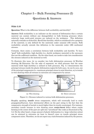
  • 1. 5.1 Chapter 5 – Bulk Forming Processes (I) Questions & Answers Slide 5.10 Question: What is the difference between bulk workability and ductility? Answer: Bulk workability is an indicator on the amount of deformation that a certain material can sustain without any damage/defect in bulk forming processes where relatively large multi-axial stresses are induced on the workpiece. This definition naturally reminds us of ductility. Recall that ductility, which is considered to be a property of the material, is only defined for the materials under uniaxial (1D) tension. Bulk workability actually extends this definition to the materials under (3D) multiaxial stresses. Certainly, there exists a correlation between bulk workability and ductility. To have “good” bulk workability, high ductility (i.e. ductile workpiece material) is the necessary (but not the sufficient) condition. On the other hand, one needs to take into consideration the stresses induced on the material as well. To illustrate this issue, let us consider two bulk deformation processes: i) Wire/bar drawing; ii) Extrusion. For the sake of argument, we shall presume that the same material (with high ductility) is utilized in both processes. Fig. 5.1 demonstrates the principal stresses inside the plastic deformation region for both cases. As can be seen, one of the principal components (i.e. maximum principal stress in axial direction, a) is tensile in wire drawing while all stresses in extrusion are compressive by nature. Fdraw σa σa σr σr σt Die Deformation Region Fext σa σa σr σr σt Deformation Region Die Ram (a) Wire drawing (b) Direct extrusion Figure 5.1: Stresses induced in various bulk deformation processes. Roughly speaking, tensile stress components, which will eventually lead to crack propagation/fracture, have detrimental effects on the part owing to the fact that the compressive strength of metals is much higher than its tensile counterpart. For instance, secondary tensile stresses in wire drawing cause center-burst defect where cracks forming at the center of the part are split into “arrowhead” like voids as illustrated in Fig. 5.2. On the other hand, a large amount of plastic deformation (i.e. large reduction ratios) can be attained in extrusion (at least in theory!) since no tensile principal stress component exists. Therefore, we do not expect any crack formation induced by the process.
  • 2. 5.2 Figure 5.2: Center-burst defect in wire drawing. Consequently, one can deduce that greater bulk workability is attained in extrusion if compared to wire drawing. It is self-evident that the ductility alone is not sufficient to define bulk workability. One needs to take into consideration the stresses induced in a particular process. For this purpose, the hydrostatic stress, which is defined as the arithmetic mean of principal stress components, is commonly utilized. More compressive the hydrostatic stress the better. To summarize, there are two necessary conditions for good bulk workability: i) High ductility (which is attributed to the material); ii) high compressive hydrostatic stress (which depends on the process itself). Slide 5.11 Question: How do we measure (or quantify) bulk workability? Answer: In the previous slide, we have qualitatively discussed bulk workability. It is obvious that bulk-workability requires a metric/measure/criteria for manufacturing engineering applications. In literature, there exist a large number of criteria to quantify bulk workability. The most common premise among them is the effect of tensile stress components (due to reasons discussed in Slide 5.10). For instance, according to Cockroft & Latham criterion, one should take a look at the work done by the highest tensile component. If this work/energy reaches a critical value, the fracture becomes eminent. In other words, as work done by the highest tensile stress component gets smaller, the onset of fracture is deferred. Hence, the bulk workability is improved. Likewise, Datko’s criterion defines a natural tensile strain. The fracture is observed when this natural strain exceed a certain threshold. For convenience, this value is taken as the tensile strain at fracture (frac) which happens to be registered in uniaxial tensile test. Slides 5.13 & 5.14 Question: How is the friction phenomenon modelled in bulk deformation processes? Answer: In cold forming, the Coulomb friction model is commonly employed due to its sheer simplicity. However, there is a minor twist in its application. To illustrate this, let us consider the case in Fig. 5.3a in which a body is pushed against friction and it starts to slide on the surface under the action of F. Hence, the shear stresses induced by the friction can be expressed as
  • 3. 5.3 𝜏𝑓 = 𝜇𝜎normal (5.1) where  denotes the coefficient of (kinetic) friction. In Eqn. (5.1), 𝜎𝑛𝑜𝑟𝑚𝑎𝑙 = 𝑃 𝐴 ; 𝐹 = 𝜏𝑓𝐴. If the friction at the interface is too high, a curious event takes place: the body adheres to the surface and the material is plastically shorn1 just above the surface. This is due to the fact that the force required to shear the material plastically is actually less than the one to overcome the friction at the interface. This case (which is referred to as stiction or sticking friction) is schematically illustrated in Fig. 5.3b. P F Area: A τf = μσnormal P F τf = τyield Area: A (a) Sliding friction (b) Sticking friction Figure 5.3: Friction models. The shear stress induced inside the body becomes 𝜏𝑓 = 𝜏yield = 𝑘 (5.2) where yield is called shear stress in yield or shear flow stress. According to Tresca’s yield criterion, 𝜏yield = 𝑘 = 𝑌𝑆/2. On the other hand, von Mises yield criterion suggests that 𝜏yield = 𝑌𝑆/√3. Notice that the material is plastically shorn here. That is, despite the fact that there is a relative motion along the shear plane (right above the surface), the cohesion in part is maintained. Consequently, we can combine Eqns. (5.1) and (5.2) to obtain a generalized friction model: 𝜏𝑓 = { 𝜇𝜎normal, 𝜇𝜎normal < 𝜏yield 𝜏yield, 𝜇𝜎normal ≥ 𝜏yield (5.3) Unfortunately, the friction model discussed above is not too suitable for hot forming. In that case, the following shear model is often times utilized: 𝜏𝑓 = 𝑚∗ 𝜏yield (5.4) where 0  m*  1 is a friction factor and should not to be confused with the strain-rate sensitivity exponent! The graph on the left (in Slide 5.14) is actually the pictorial description of Eqn. (5.3). Assume that the normal stress (normal) is constantly increasing. The graph shows how the shear stress (f) changes for different  values. When normal < yield, the material slides on the surface (i.e. sliding friction is in effect). Similarly, if normal goes beyond yield, the 1 Verb: to shear; Past tense: sheared; Past participle: shorn.
  • 4. 5.4 shear stress saturates at yield no matter how big normal is. From this point on, the stiction kicks in and the material is plastically shorn inside. Similarly, the graph on the right (in Slide 5.14) depicts the upper bound of  where the sliding friction is still in effect. That is, when maxnormal = yield, we reach to a boundary point where stiction begins to take over. Assuming that yield = YS/2 (Tresca Yield Criterion), we calculate 𝜇max = 𝑌𝑆 2𝜎normal (5.5) The graph plots max as a function of normal. If the  values below the curve are chosen, the sliding friction gets to be always effective. Question: In Slide 5.13, it appears as if the shear flow stress (𝜏yield = 𝑘) is 𝑌𝑆/2 according to Tresca while it is taken as 𝑌𝑆/√3 when von Mises yield criterion is considered. Why do they differ? After all, wouldn’t it make more sense if 𝜏yield were treated as an intrinsic material property like YS? Answer: Let us start our discussion with the computation of 𝜏yield ≜ 𝑘. Consider the principal stress states shown in Fig. 5.4. Here, the Mohr’s circles represent planar pure shear-stress case where 𝜎1 = 𝑘; 𝜎2 = 0; 𝜎3 = −𝑘. The application of Tresca’s yield criterion to this particular case will give rise to 𝜎1 − 𝜎3 = 𝑌𝑆 ∴ 𝑘 − (−𝑘) = 𝑌𝑆 ⟹ 𝑘 = 𝑌𝑆 2 (5.6) Similarly, when von Mises yield criterion is used, we get 𝜎𝑒𝑞 = √ (𝜎1 − 𝜎2)2 + (𝜎2 − 𝜎3)2 + (𝜎3 − 𝜎1)2 2 = 𝑌𝑆 √ (𝑘 − 0)2 + [0 − (−𝑘)]2 + (−𝑘 − 𝑘)2 2 = 𝑌𝑆 ∴ √ 6𝑘2 2 ⟹ 𝑘 = 𝑌𝑆 √3 (5.7) For this special instance, the shear stress in yield (i.e. k) should be interpreted as the magnitude of the pure shear stress induced as the material commences to yield. Not surprisingly, k differs slightly owing to the fact that the yield boundaries considered by the above-mentioned criteria are different (please see Slide 3.36 and the corresponding Q&A comment). In other words, the discrepancy in k is mainly attributed to the difference between two yield criteria on when the material will start to deform plastically2. Consequently, the shear-stress in yield cannot be treated as an intrinsic material property like YS. 2 The procedure for the calculation of the maximum shear stress in the material (i.e. Mohr’s method) is essentially the same for both methods.
  • 5. 5.5 σ τ σ1 = k σ2 = 0 σ3 = -k τmax τmax τmax σ1 σ1 σ3 σ3 σ2 = 0 Figure 5.4: Planar pure shear-stress case. Slides 5.22-5.30 Question: What is the general force model for plain-strain upsetting at room temperature? Answer: Let us combine the models presented in these slides to compute the overall punch force as a function of upsetting height (h). The pressure distribution at the workpiece-die interface for plain-strain case can be summarized as follows: 𝑝(𝑥) 𝑌𝑆 = { 𝑎 − 𝑥 ℎ + 1 2𝜇 [1 + ln(2𝜇)], 0 ≤ 𝑥 ≤ 𝑥1 𝑒 2𝜇 ℎ (𝑎−𝑥) , 𝑥1 < 𝑥 ≤ 𝑎 (5.8) Here, the length of the stiction region is 𝑥1 = 𝑎 + ℎ 2𝜇 ⋅ ln(2𝜇) (5.9) Thus, integrating the pressure in Eqn. (5.8) over the contact area yields the desired force: 𝐹 = 2 ∫ 𝑝(𝑥)𝑤 𝑎 0 𝑑𝑥 (5.10) That is, 𝐹 2 ∙ 𝑌𝑆 ∙ 𝑤 = ∫ { 𝑎 − 𝑥 ℎ + 1 2𝜇 [1 + ln(2𝜇)]} 𝑥1 0 𝑑𝑥 + ∫ 𝑒 2𝜇 ℎ (𝑎−𝑥) 𝑎 𝑥1 𝑑𝑥 (5.11)
  • 6. 5.6 where w refers to the width of the workpiece (i.e. the dimension of the workpiece into the paper plane). When Eqn. (5.11) is evaluated, we obtain 𝐹 𝑌𝑆 ∙ 𝑤 ∙ ℎ = | 𝑥 ℎ { 2𝑎 − 𝑥 ℎ + 1 𝜇 [1 + ln(2𝜇)]} | 0 𝑥1 + | 1 𝜇 𝑒 2𝜇 ℎ (𝑎−𝑥) | 𝑎 𝑥1 (5.12) Here, x1  0; 𝑌𝑆 ≅ 𝜎𝑓 = 𝐾(𝜀𝑒𝑞) 𝑛 and 𝜀𝑒𝑞 = 𝑙𝑛 ( ℎ0 ℎ ). It is tempting to simplify Eqn. (5.12) by plugging in the integration limits. However, the simplified expression obscures the physical interpretation while failing to produce meaningful results when x1 < 0. Question: How is the last expression in Slide 5.25 obtained? Answer: First, let us recall the (Maclaurin) series expansion of exponential function: 𝑒𝑥 = 1 + 𝑥 1! + 𝑥2 2! + 𝑥3 3! + ⋯ (−∞ < 𝑥 < ∞) (5.13) If we use only first three terms (including quadratic one) in Eqn. (5.13), the average interface pressure can be approximated as 𝑝𝑎𝑣 𝑌𝑆 = ℎ 2𝜇𝑎 [1 + 2𝜇𝑎 1! ℎ + (2𝜇𝑎)2 2! ℎ2 ⏟ ≈ 𝑒(2𝜇𝑎)/ℎ − 1] (5.14) Consequently, Eqn. (5.14) boils down to the given result in the slide: 𝑝𝑎𝑣 𝑌𝑆 ≅ 1 + 𝜇 𝑎 ℎ (5.15) Slides 5.35-5.38 Question: What is the general force model for upsetting an axisymmetric workpiece at room temperature? Answer: Recall that the models for different friction conditions were partially developed in the course slides. Following the procedure presented in Slides 5.22-5.30, one can combine them into a general mathematical model. For sliding friction, the pressure distribution on the punch was found as follows (see Slide 5.38): 𝑝(𝑟) 𝑌𝑆 = 𝑒 2𝜇 ℎ (𝑅−𝑟) (5.16) For sticking friction (where 𝜏𝑓 = 𝜏𝑦𝑖𝑒𝑙𝑑 ≅ 𝑌𝑆 2 ), the differential equation representing the radial force balance takes the following form (please refer to Slide 5.35): 𝑑𝜎𝑟 = 𝑌𝑆 𝑑𝑟 ℎ (5.17) Since 𝑑𝜎𝑟 = −𝑑𝑝, the integration of the resulting equation yields 𝑝 = −𝑌𝑆 𝑟 ℎ + 𝑐 (5.18)
  • 7. 5.7 Notice that the boundary condition (BC) is p = YS when r = R. With this BC, the integration constant c can be directly determined (see Slide 5.38). Thus, the overall solution for this case becomes 𝑝(𝑟) 𝑌𝑆 = 1 + 𝑅 − 𝑟 ℎ (5.19) Notice that Eqn. (5.19) incorporates the assumption that the whole surface is sticking. Now, we can roll these models into one. Just like the plane-strain upsetting, the central (i.e. core) portion of the workpiece (within a radius of r1) is expected to stick onto the surface of the punch while the material elsewhere is to slide. Before we proceed, let us first determine the radius of the sticking zone. At r = r1, the frictional shear stress computed via Eqn. (5.16) must reach the shear stress in yield. That is, 𝜏𝑓 = 𝜇 ⋅ 𝑝(𝑟1) = 𝜏𝑦𝑖𝑒𝑙𝑑 ≅ 𝑌𝑆 2 (5.20a) ∴ 𝜇 ⋅ 𝑌𝑆 ⋅ 𝑒 2𝜇 ℎ (𝑅−𝑟1) ≅ 𝑌𝑆 2 (5.20b) Solving Eqn. (5.20b) for r1 gives 𝑟1 = 𝑅 + ℎ 2𝜇 ln(2𝜇) (5.21) In the core section (where 0 ≤ 𝑟 ≤ 𝑟1), Eqn. (5.19) cannot be employed directly owing to the fact its BC must be updated so as to switch smoothly to the sliding friction at r = r1. Therefore, the integration constant in Eqn. (5.18) should be re-evaluated so that the pressure given by Eqn. (5.18) at this boundary must be equal to the one calculated via Eqn. (5.16). Otherwise, there will be discontinuity at r = r1. Consequently, −𝑌𝑆 𝑟1 ℎ + 𝑐 ⏟ Eqn. (5.18) = 𝑌𝑆 ⋅ 𝑒 2𝜇 ℎ (𝑅−𝑟1) ⏟ Eqn. (5.16) (5.22) Solving c gives rise to 𝑐 = 𝑌𝑆 ℎ [𝑅 + ℎ 2𝜇 (ln(2𝜇) + 1)] (5.23) Plugging Eqn. (5.23) into Eqn. (5.18) yields 𝑝(𝑟) 𝑌𝑆 = 𝑅 − 𝑟 ℎ + 1 2𝜇 [ln(2𝜇) + 1] (5.24) To summarize, the general pressure model becomes 𝑝(𝑟) 𝑌𝑆 = { 𝑅 − 𝑟 ℎ + 1 2𝜇 [1 + ln(2𝜇)], 0 ≤ 𝑟 ≤ 𝑟1 𝑒 2𝜇 ℎ (𝑅−𝑟) , 𝑟1 < 𝑟 ≤ 𝑅 (5.25) Recall that 𝑌𝑆 ≅ 𝜎𝑓 = 𝐾(𝜀𝑒𝑞) 𝑛 while 𝜀𝑒𝑞 = 𝑙𝑛 ( ℎ0 ℎ ). The upsetting force is simply obtained by integrating Eqn. (5.25) over the surface in contact:
  • 8. 5.8 𝐹 2𝜋 𝑌𝑆 = ∫ { 𝑅 − 𝑟 ℎ + 1 2𝜇 [1 + ln(2𝜇)]} 𝑟1 0 𝑟𝑑𝑟 + ∫ 𝑒 2𝜇 ℎ (𝑅−𝑟) 𝑅 𝑟1 𝑟𝑑𝑟 (5.26) Hence, when Eqn. (5.26) is evaluated, we get 𝐹 𝜋𝑅2𝑌𝑆 = | 𝑟2 𝑅2 { 3𝑅 − 2𝑟 3ℎ + 1 2𝜇 [1 + ln(2𝜇)]} | 0 𝑟1 + | 1 2(𝜇𝑅)2 ℎ(ℎ + 2𝜇𝑟)𝑒 2𝜇 ℎ (𝑅−𝑟) | 𝑅 𝑟1 (5.27) Notice that Eqn. (5.27) is valid for 𝑟1 ≥ 0. Otherwise (𝑟1 < 0), the total surface slide condition will be in effect. In such a case, 𝑟1 should be taken as 0 in the integration limits of Eqn. (5.27). Consequently, that equation boils down to the expression in Slide 5.38: 𝐹 = 2𝜋𝑅2 𝑌𝑆 ( ℎ 2𝜇𝑅 ) 2 (𝑒 2𝜇𝑅 ℎ − 2𝜇𝑅 ℎ − 1) (5.28) Question: So far, we have mostly restricted our attention to cold-upsetting. How can we adopt our models to hot-working as well? Answer: In hot-working, the yield strength of the material depends on the temperature and the prevailing strain-rate. Furthermore, the friction between the hot workpiece and the die attains a different nature. In practice, two methods are commonly employed to model hot-upsetting process: Method I The general model given above can be directly employed except that the effective kinetic friction coefficient is artificially increased to high values ( = 0.4…0.5)3 owing to the fact that the hot metal is likely to stick to the punch surface. Therefore, the upsetting force could be computed utilizing Eqn. (5.27) that makes good use of the composite friction model. However, the yield strength in Eqn. (5.27) has to be estimated via 𝑌𝑆 ≅ 𝜎𝑓 = 𝐶(𝜀̇)𝑚 (5.29) where the equivalent strain-rate is defined as 𝜀̇ = 𝑑𝜀 𝑑𝑡 = 𝑑𝜀 𝑑ℎ ⋅ 𝑑ℎ 𝑑𝑡 (5.30) It is critical to note that since the upsetting height is decreasing (i.e. dh < 0), the punch velocity (i.e. dh/dt) needs to be taken as a negative quantity to be consistent in the derivation. Therefore, Eqn. (5.30) becomes 𝜀̇ = 𝑑 𝑑ℎ [𝑙𝑛 ( ℎ0 ℎ )] ⏟ −1/ℎ 𝑑ℎ 𝑑𝑡 ⏟ −𝑣𝑝𝑢𝑛𝑐ℎ = 𝑣𝑝𝑢𝑛𝑐ℎ ℎ (5.31) Method II This method adapts the shear model of friction (see Slide 5.13). This time, the sticking friction model, which has a close correspondence to the shear model, can be directly utilized. Recall that in the shear model, the frictional shear stress is presumed to be 3 For instance, see Table 17.1 of Ref. [1].
  • 9. 5.9 independent of the pressure at the interface. Hence, one can visualize that the hot metal is plastically shorn over the whole punch surface. Consequently, the Eqn. (5.18) becomes 𝑝 = −𝑚∗ 𝑌𝑆 𝑟 ℎ + 𝑐 (5.32) where m* is the friction factor. The boundary condition is again p = YS when r = R. Thus, finding the integration constant c and plugging the result into Eqn. (5.32) yields 𝑝(𝑟) 𝑌𝑆 = 1 + 𝑚∗ 𝑅 − 𝑟 ℎ (5.33) The upsetting force is simply obtained by integrating Eqn. (5.33) over the whole punch surface: 𝐹 𝑌𝑆 = ∫ (𝑚∗ 𝑅 − 𝑟 ℎ + 1) 𝑅 0 2𝜋𝑟𝑑𝑟 (5.34) When Eqn. (5.34) is evaluated, we obtain 𝐹 𝑌𝑆 = 𝜋𝑅2 (1 + 𝑚∗ 𝑅 3ℎ ) (5.35) Question: How about upsetting a ring? Is it possible to employ the solution given in Slides 5.35-5.38? Answer: Certainly. Let us focus on the Coulomb friction case. If the solution given in the Slide 5.38 is examined, one realizes that there is only one integration constant but there are two boundary conditions in the ring case. As a solution, we divide the ring into two regions as shown in Fig. 5.5. In the first region, the material is flowing outwards while the flow direction in the second one is towards the center (i.e. inwards). It is self-evident that there should be a neutral surface in between the adjacent regions where the relative (radial) speed of the material with respect to the punch is essentially zero. For the first region, the solution given in Slide 5.37 can be directly employed. The new boundary condition in this case is 𝑝|𝑟=𝑟0 = 𝑌𝑆 (5.36) The corresponding integration constant becomes 𝑐 = ln(𝑌𝑆) + 2𝜇𝑟0 ℎ (5.37) Evidently, the pressure distribution for Region I takes the following form: 𝑝(𝑟) 𝑌𝑆 = 𝑒 2𝜇(𝑟0−𝑟) ℎ (5.38) where 𝑟𝑛 ≤ 𝑟 ≤ 𝑟0. With respect to the second region, the presented solution must be modified a little bit owing to the fact that the friction force must change its direction to resist the material’s motion which is headed inwards. Consequently, the altered solution can be expressed as ln(𝑝) = 2𝜇𝑟 ℎ + 𝑐 (5.39)
  • 10. 5.10 Similarly, the boundary condition for this region becomes 𝑝|𝑟=𝑟𝑖 = 𝑌𝑆 (5.40) We can now obtain the integration constant: 𝑐 = ln(𝑌𝑆) − 2𝜇𝑟𝑖 ℎ (5.41) Substituting Eqn. (5.41) into (5.39) gives the pressure distribution for Region II: 𝑝(𝑟) 𝑌𝑆 = 𝑒 2𝜇(𝑟−𝑟𝑖) ℎ (5.42) where 𝑟𝑖 ≤ 𝑟 ≤ 𝑟𝑛. Notice that on the neutral circle, Eqns. (5.38) and (5.42) must yield the same pressure otherwise there would be jump in the pressure at this transition point. In fact, this continuity condition allows us to determine the location of the neutral surface: 𝑒 2𝜇(𝑟0−𝑟𝑛) ℎ = 𝑒 2𝜇(𝑟𝑛−𝑟𝑖) ℎ (5.43) Consequently, 𝑟𝑛 = 𝑟0 + 𝑟𝑖 2 (5.44) Question: While upsetting a ring, how do we determine the dimensions of the workpiece (i.e. ri and ro) at a particular upsetting height (h)? Answer: For this purpose, we shall employ the principle of volume/mass conservation. For Region I (see Fig. 5.5), the input flow rate must be equal to the output flow rate of the material. That is, 𝑣𝑝𝜋(𝑟0 2 − 𝑟𝑛 2) = 𝑣02𝜋𝑟0ℎ (5.45a) ∴ 𝑑𝑟0 𝑑𝑡 = 𝑣0 = 𝑣𝑝 𝑟0 2 − 𝑟𝑛 2 2𝑟0ℎ (5.45b) where the punch velocity is defined as 𝑣𝑝 = 𝑑ℎ 𝑑𝑡 = constant. Similarly, for Region II, the continuity equation becomes 𝑑𝑟𝑖 𝑑𝑡 = 𝑣𝑖 = 𝑣𝑝 𝑟𝑛 2 − 𝑟𝑖 2 2𝑟𝑖ℎ (5.46) The (coupled/nonlinear) ordinary differential equations (5.45b) and (5.46) must be solved simultaneously to obtain 𝑟0 and 𝑟𝑖 as a function of either time or upsetting height. Note that finding an analytical solution to these differential equations is quite difficult. Therefore, numerical solutions are oftentimes accommodated in practice. To that end, the backward Euler method could be employed to express them as finite-difference equations: 𝑑𝑟0 𝑑𝑡 ≈ 𝑟0(𝑘) − 𝑟0(𝑘 − 1) Δ𝑇 = 𝑣𝑝 𝑟0 2 (𝑘 − 1) − 𝑟𝑛 2 (𝑘 − 1) 2𝑟0(𝑘 − 1)ℎ(𝑘 − 1) (5.47a)
  • 11. 5.11 ∴ 𝑟0(𝑘) = 𝑟0(𝑘 − 1) + 𝑣𝑝Δ𝑇 ⏟ Δℎ 4𝑟0 2 (𝑘 − 1) − [𝑟0(𝑘 − 1) + 𝑟𝑖(𝑘 − 1)]2 8𝑟0(𝑘 − 1)ℎ(𝑘 − 1) (5.47b) where k = 1, 2, … refers to the iteration/time index; Δ𝑇 is the integration time step; Δh = 𝑣𝑝Δ𝑇 is the corresponding increment in the height. Following the same steps, Eqn. (5.46) becomes 𝑟𝑖(𝑘) = 𝑟𝑖(𝑘 − 1) − Δℎ [𝑟0(𝑘 − 1) + 𝑟𝑖(𝑘 − 1)]2 − 4𝑟𝑖 2 (𝑘 − 1) 8𝑟𝑖(𝑘 − 1)ℎ(𝑘 − 1) (5.48) Similarly, the height equation can be expressed as follows: ℎ(𝑘) = ℎ(𝑘 − 1) − Δℎ (5.49) Here, the initial conditions are set as 𝑟0(0) = 𝑅0; 𝑟𝑖(0) = 𝑅𝑖; ℎ(0) = 𝐻0. Notice that as a simple approximation, one can compute 𝑟0 and 𝑟𝑖 by assuming that the radius of neutral surface is constant: 𝑟𝑜 + 𝑟𝑖 = 𝑅0 + 𝑅𝑖 (5.50) Similarly, using volume constancy, we have 𝜋(𝑟𝑜 2 − 𝑟𝑖 2 )ℎ = 𝜋(𝑅𝑜 2 − 𝑅𝑖 2 )𝐻𝑜 (5.51) Simultaneously solving 𝑟0 and 𝑟𝑖 from Eqns. (5.50) and (5.51) leads to 𝑟𝑜(ℎ) = 𝑅0 + 𝑅𝑖 2 + 𝑅0 − 𝑅𝑖 2 ⋅ 𝐻𝑜 ℎ (5.52a) 𝑟𝑖(ℎ) = 𝑅0 + 𝑅𝑖 2 − 𝑅0 − 𝑅𝑖 2 ⋅ 𝐻𝑜 ℎ (5.52b) The MATLAB Script given in Table 5.1 performs the above-mentioned computations. The output of the script is shown in Fig. 5.6. The dotted lines illustrate the approximated quantities in Eqn. (5.52). As can be seen, the approximation generally yields acceptable results. r0 ri Punch Anvil h vp rn vi v0 Region I Region II Figure 5.5: Nomenclature for ring upsetting. Figure 5.6: Numerical integration results for ring upsetting case. 60 65 70 75 80 85 90 95 100 130 140 150 160 170 180 190 200 210 220 Upsetting height, h [mm] Radius [mm] r0 ri rn
  • 12. 5.12 It is critical to notice that the solution provided here harbors the implicit assumption that the friction at the workpiece-die interface is negligible. This is obviously not the case in practice. To have a realistic solution, one needs to take into account the flow rule (i.e. Levy-Mises rule) and solve the resulting ordinary differential equation set accordingly. Table 5.1 MATLAB script to compute the dimensions of the ring while upsetting. Ro = 200; Ri = 150; Ho = 100; Hf = 60; dh = .001; N = ceil((Ho-Hf)/dh); ro = zeros(N,1); ri = zeros(N,1); roa = ro; ria = ri; h = zeros(N,1); ro(1) = Ro; ri(1) = Ri; roa(1) = Ro; ria(1) = Ri; h(1) = Ho; for k = 2:N rn = (ro(k-1) + ri(k-1))/2; dr0 = (ro(k-1)^2 - rn^2)*dh/(2*ro(k-1)*h(k-1)); dri = (rn^2 - ri(k-1)^2)*dh/(2*ri(k-1)*h(k-1)); ro(k) = ro(k-1) + dr0; ri(k) = ri(k-1) - dri; h(k) = h(k-1) - dh; roa(k) = .5*(Ro+Ri) + .5*(Ro-Ri)*Ho/h(k); ria(k) = .5*(Ro+Ri) - .5*(Ro-Ri)*Ho/h(k); end close all plot(h,[ro ri (ro+ri)/2]); hold on plot(h,[roa ria (roa+ria)/2],':'); grid xlabel('Upsetting height, h [mm]') ylabel('Radius [mm]') legend('r_0','r_i','r_n') Slide 5.46 Question: What is the neutral point in rolling? Answer: The neutral point (NP) (also known as no-slip point) is a special location on the roll where no frictional force exist as the relative horizontal speed of the material with respect to the roll is essentially zero. Recall that friction force only develops when there is a relative motion between two bodies in contact. Note that the friction force on the left hand of the NP actually pulls in the material towards the deformation zone due to the fact that the horizontal velocity of the roll is much faster than the material itself. Similarly, on the right hand side of the NP, the friction force develops to oppose the material’s motion since the horizontal speed of the material now exceeds the one associated with the roll. For all practical purposes, the friction forces (in opposition) on both sides of the NP are assumed to be equal in magnitude.
  • 13. 5.13 Question: How is the location of the neutral point on the roll is determined? Answer: To find the location of neutral point (NP), let us consider the kinematic model shown in Fig. 5.7. We shall presume that the velocity of the material at the inlet (v0) is initially known. h0/2 h1/2 hn/2 βn R Ω n Roll vroll Deformation Region v0 v1 O A B x y Figure 5.7: Nomenclature for rolling process. Using the roll geometry given in the figure, the distance |OB| can be calculated: |𝑂𝐵| = 𝑅 + ℎ1 2 = 𝑅 ⋅ 𝑐𝑜𝑠(𝛽𝑛) ⏟ |𝑂𝐴| + ℎ𝑛 2 ⏟ |𝐴𝐵| (5.53a) ∴ 2𝑅 + ℎ1 = 2𝑅 𝑐𝑜𝑠(𝛽𝑛) + ℎ𝑛 (5.53b) By definition, the horizontal speed of the material (vn) at NP is equal to that of the roll (vroll x ): 𝑣𝑟𝑜𝑙𝑙 𝑐𝑜𝑠(𝛽𝑛) ⏟ 𝑣𝑟𝑜𝑙𝑙 𝑥 = 𝑣0ℎ0 ℎ𝑛 ⏟ 𝑣𝑛 (5.54) Here, the circumferential speed of the roll (vroll) is 𝑣𝑟𝑜𝑙𝑙 = 𝑅Ω (5.55) where  denotes the angular speed of the roll [rad/s]. Thus, Eqn. (5.54) can be rearranged as 𝑐𝑜𝑠(𝛽𝑛) = 𝑣0ℎ0 𝑅Ωℎ𝑛 (5.56) Substituting Eqn. (5.56) into (5.53b) yields a quadratic equation of hn: ℎ𝑛 2 − (2𝑅 + ℎ1)ℎ𝑛 + 2𝑣0ℎ0 Ω = 0 (5.57) Since h1 ≤ hn ≤ h0, the feasible root of Eqn. (5.57) leads to the location of NP:
  • 14. 5.14 ℎ𝑛 = 𝑅 + ℎ1 2 − √(𝑅 + ℎ1 2 ) 2 − 2𝑣0ℎ0 Ω (5.58) The derivation above presumes that v0 is known beforehand. Unfortunately, this is not a viable assumption. In practice, v0 is the sought-after quantity (rather hn itself). Note that v0 is affected by many factors such as , , geometric parameters (R, w, h0, h1), and material properties (K, n, f0). Thus, the pressure distribution around the roll is first computed using numerical- or (simplified) analytical techniques. The pressure attains its maximum value at hn (for instance, see Fig. 18.4 of Ref. [1]). Once hn is found, v0 is estimated subsequently using Eqn. (5.57). In fact, Ref. [3] presents the location of the neutral point (or the neutral plane to be exact!) directly4 using the coordinate frame in Fig. 5.7: 𝑥𝑛 = 𝑥1 2 (1 + 𝑥1 2𝑅𝜇 ) + 𝜎𝑥0ℎ0 − 𝜎𝑥1ℎ1 4𝜎𝑓𝑚𝜇 (5.59) where 𝑥𝑛 and 𝑥1 denote the horizontal positions of the neutral point and the outlet respectively; 𝜎𝑥0 ≡ 𝜎𝑏𝑡 and 𝜎𝑥1 ≡ 𝜎𝑓𝑡 refer to the back- and the front tensions applied to the workpiece (Slide 5.53) while 𝜎𝑓𝑚 indicates the mean flow stress inside the deformation zone (see Slides 5.17 & 5.49). Referring to the right triangle (OAC) in Fig. 5.8, the horizontal position of the outlet can be estimated: 𝑥1 2 ⏟ |𝐴𝐶|2 + (𝑅 − ℎ0 − ℎ1 2 ) 2 ⏟ |𝑂𝐴|2 = 𝑅2 ⏟ |𝑂𝐶|2 (5.60a) ∴ 𝑥1 = √𝑅(ℎ0 − ℎ1) ⏟ 𝐿2 − (ℎ0 − ℎ1)2 4 ⏟ neglect ≈ 𝐿 (5.60b) Here, L = √𝑅(ℎ0 − ℎ1) indicates the approximate length of the deformation region (see also Slide 5.48). Employing the geometry given in Fig. 5.7, the thickness of the material at a particular position (x) could be calculated: ℎ(𝑥) = ℎ1 + 2𝑅 − 2√𝑅2 − (𝑥1 − 𝑥)2 (5.61) where 0 ≤ 𝑥 ≤ 𝑥1. Substituting Eqns. (5.59) and (5.60b) into (5.61) yields ℎ𝑛 ≜ ℎ(𝑥𝑛): ℎ𝑛 − ℎ1 2𝑅 = 1 − √1 − ( 𝐿 − 𝑥𝑛 𝑅 ) 2 (5.62) Given  and ℎ𝑛, one can determine the inlet speed (v0) by rearranging Eqn. (5.57): 𝑣0 = 𝑅Ω ℎ𝑛 ℎ0 (1 − ℎ𝑛 − ℎ1 2𝑅 ) (5.63) 4 See Section 4.1 of Ref. [3].
  • 15. 5.15 Slide 5.47 Question: What is initial grasp/grip? Answer: The initial grip yields the condition for both initiating and sustaining material feed/flow in flat rolling process with the help of friction. As derived in the slide, the condition is tan(𝛼) = sin(𝛼) cos(𝛼) ≤ 𝜇 (5.64) where  is referred to as angle of bite. Using the geometry in Fig. 5.8, the cosine of this angle can be written: cos(𝛼) = 1 − ℎ0 − ℎ1 2𝑅 = 1 − 𝑑 2𝑅 (5.65) Here, d ≜ h0 − ℎ1 is called the draft which represents the thickness reduction in flat rolling. h0/2 h1/2 α R Roll O A B C Figure 5.8: Geometry for initial grasp. In fact, we need a more utilitarian condition than Eqn. (5.64). To this end, sin() can be obtained by employing the (right) triangle (OAC) in Fig. 5.8: sin(𝛼) = √𝑅2 − (𝑅 − 𝑑/2)2 𝑅 ≅ √𝑑/𝑅 (5.66) Substituting Eqns. (5.65) and (5.66) into (5.64) simply gives √𝑑/𝑅 1 − 𝑑 2𝑅 ≤ 𝜇 (5.67) If Eqn. (5.67) is rearranged and simplified, we get 𝑑 𝑅 ≤ 𝜇2 1 + 𝜇2 (5.68) Consequently, the maximum draft (i.e. maximum possible reduction in thickness) takes the following form:
  • 16. 5.16 𝑑𝑚𝑎𝑥 = 𝜇2 𝑅 1 + 𝜇2 (5.69) Notice that if 2 is neglected in the denominator, Eqn. (5.69) boils down to 𝑑𝑚𝑎𝑥 = 𝜇2 𝑅 (see Eqn. (18.18) in Ref. [1])5. Slide 5.48 Question: What are the factors involved in rolling force computation? Answer: The most important factors can be listed as follows: 1) Area of the deformation zone (Lw); 2) Mean flow stress of the workpiece material (fm); 3) Pressure correction factor (Q) that depends on the plastification state of the material inside the deformation zone. The roll-force is roughly the product of the abovementioned factors. It is critical to notice that flat rolling process somewhat resembles the plane-strain indentation (see Slide 5.40). However, the indenter tool happens to be cylindrical in this special case. Not surprisingly, the roll-force model in this slide bears a resemblance to the expressions in Slide 5.40 (especially, Cases II & III). Now let us elaborate these factors above: 1) While computing the area (see Slide 5.45), the area of the roll in contact with workpiece needs to be considered [i.e. (R)w where  is the angle of bite defined previously]. For the sake of simplicity, this arc length (R) is approximated as a line (i.e. the hypotenuse of the triangle shown in the slide): Rα ≅ L = √𝑅(ℎ0 − ℎ1) = √𝑅𝑑. This is a valid assumption when R >> d. 2) Since rolling is a steady-state (time-invariant) process, mean flow stress can be conveniently employed for this purpose. We shall come back to this issue on the next slide. 3) The pressure factor Q depends on the type of deformation as illustrated in Fig. 5.9. As stated in this slide, there are two different modes driven basically by the geometric parameters: i) Partial plastification (hmean/L > 1 implies thick plates + small “R”); ii) Full plastification (hmean/L  1 implies thin plates + large “R”). 5 This result could be also obtained with the utilization of Eqn. (5.67): the term (d/2R) in the denominator is usually a very small quantity and could be neglected for all practical purposes.
  • 17. 5.17 Roll Deformation Region Roll Deformation Region (a) Partial plastification (b) Full plastification Figure 5.9: Deformation modes in flat rolling. Question: We see the magic number 1.15 popping up in various places including the roll- force computation. What is the origin of this number? Answer: That number is actually 2/√3. For plane strain cases (such as upsetting, indentation, rolling, etc.) where the deformation is restrained in one particular direction6, von Mises yield criterion takes the following form (for instance, see Chapter 5.1.4 of Ref. [2]): σ1 − σ3 = 2 √3 YS = 1.15 ⋅ YS (5.70) The number 1.15 here often times shows up in subsequent derivations. Slide 5.49 Question: How is the mean flow stress computed? Answer: For cold-forming, the derivation can be found in Slide 5.17. With respect to hot- forming, the average equivalent strain-rate (𝜀̇𝑒𝑞) should be estimated. For this purpose, the following approximation comes handy: 𝜀̇𝑒𝑞 = 𝑑𝜀𝑒𝑞 𝑑𝑡 ≅ Δ𝜀𝑒𝑞 Δ𝑡 (5.71) To compute eq, we shall consider the strains inflicted at the beginning- and at the end of the deformation region: Δ𝜀𝑒𝑞 ≅ 𝑙𝑛 ( ℎ0 ℎ1 ) ⏟ exit − 0 ⏟ inlet = 𝑙𝑛 ( ℎ0 ℎ1 ) = 𝜀𝑒𝑞 (5.72) Similarly, the material’s transport time between the inlet- and the exit of the deformation zone is considered to determine t. Assuming that the length of the deformation region is L and the average speed of the material is vmean, we get Δ𝑡 ≅ 𝐿 𝑣mean = √𝑅(ℎ0 − ℎ1) 𝑣mean (5.73) The mean (average) velocity can then be calculated as 6 In such situations, the median principal stress component is taken as 𝜎2 = 𝜎1+𝜎3 2 .
  • 18. 5.18 𝑣mean = 1 ℎ1 − ℎ0 ∫ 𝑣0ℎ0 ℎ 𝑑ℎ = 𝑣0ℎ0 ℎ0 − ℎ1 ℎ1 ℎ0 𝑙𝑛 ( ℎ0 ℎ1 ) = 𝑣0ℎ0𝜀𝑒𝑞 ℎ0 − ℎ1 (5.74) Combining Eqns. (5.71) through (5.74) yields 𝜀̇𝑒𝑞 ≅ 𝑣0ℎ0𝜀𝑒𝑞 2 √𝑅(ℎ0 − ℎ1)3 (5.75) Consequently, the mean flow stress in hot-forming becomes 𝜎𝑓𝑚 = 𝐶(𝜀̇𝑒𝑞) 𝑚 (5.76) Slide 5.55 Question: What is a cambered roll? Answer: As highlighted in Slide 5.52, the rolls will elastically bend under the action of rolling forces7. Due to the elastic deformation of the rolls along their main axes, the rolled products (compressed between the rolls) will deviate significantly from the desired profile. That is, the thickness of the sheet / plate right at the center will be greater than those at the sides. As a remedy, the shape of the rolls are modified such that as they bend, the deformed shape will get to be perfectly flat. In such a scheme, the overall shape of the modified roll resembles a barrel and is called cambered roll as shown in this slide. Roughly speaking, the deflection curve of the roll is utilized as a guide to increase the diameter of the roll at a particular location along its axis. This is actually a double-edged sword: if the design is not properly done, the cambered rolls along with their new deflection curve will entirely change the pressure distribution inside the plastic deformation region. Slides 5.56 and 5.57 show the defects caused by improper cambered rolls. References [1] Groover, M. P., Fundamentals of Modern Manufacturing, 5th Edition, John Wiley, NY, 2013. [2] Tlusty, G., Manufacturing Processes and Equipment, Prentice Hall, NJ, 2000. [3] Lange, K., Lehrbuch der Umformtechnik, Band 2, Springer-Verlag, Berlin, 1975. 7 In practice, it is not possible to avoid such deformations owing to the fact that the machine elements will always have finite stiffness/rigidity.