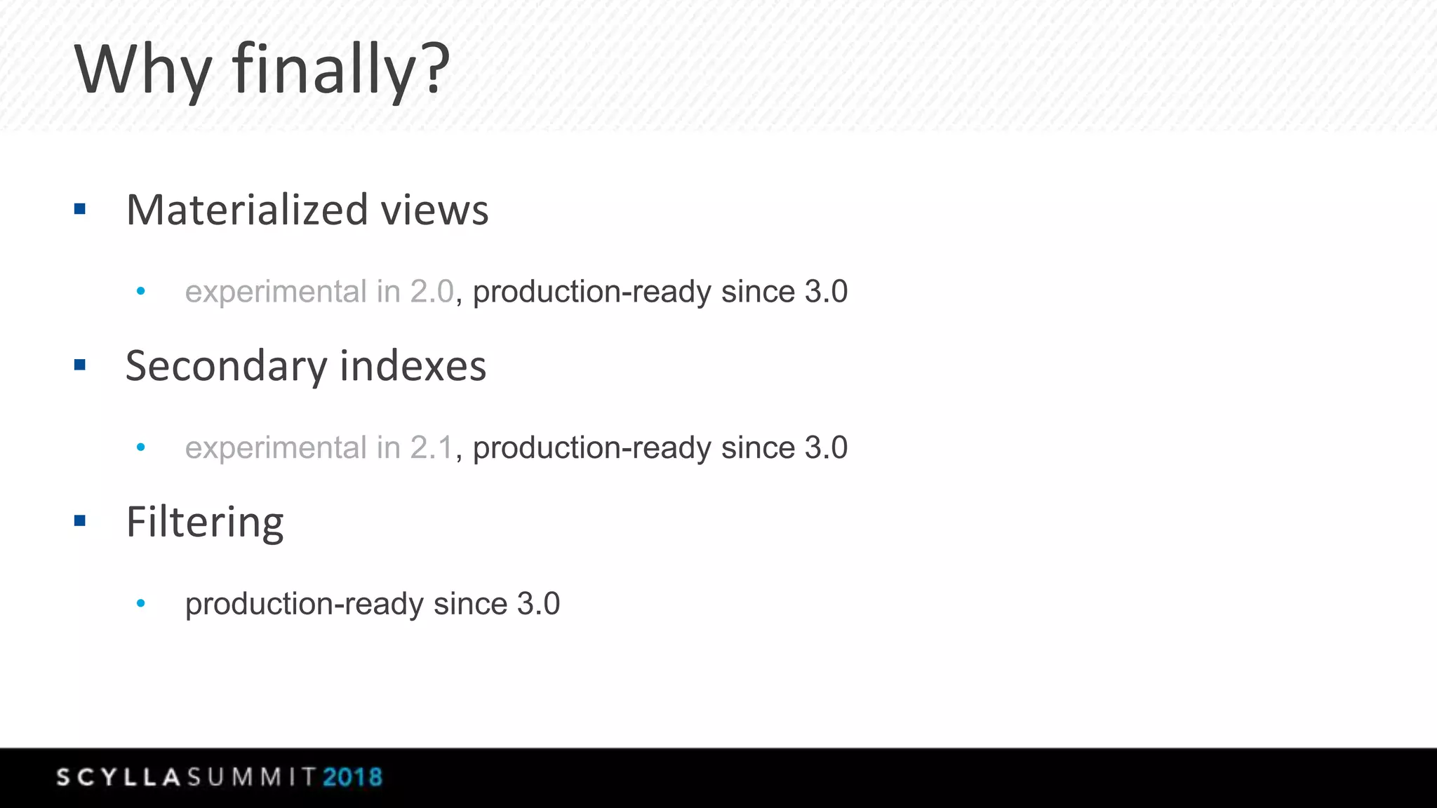
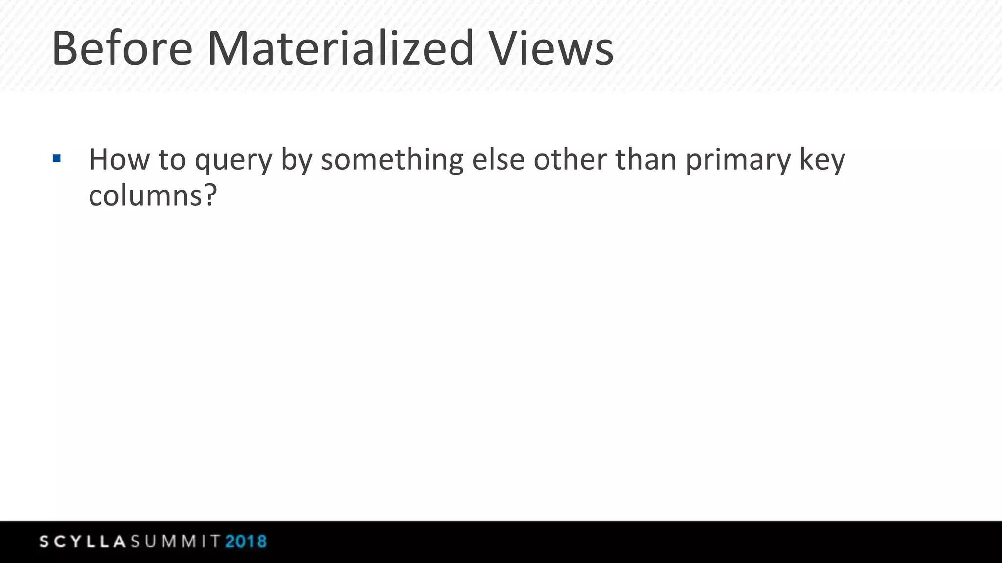
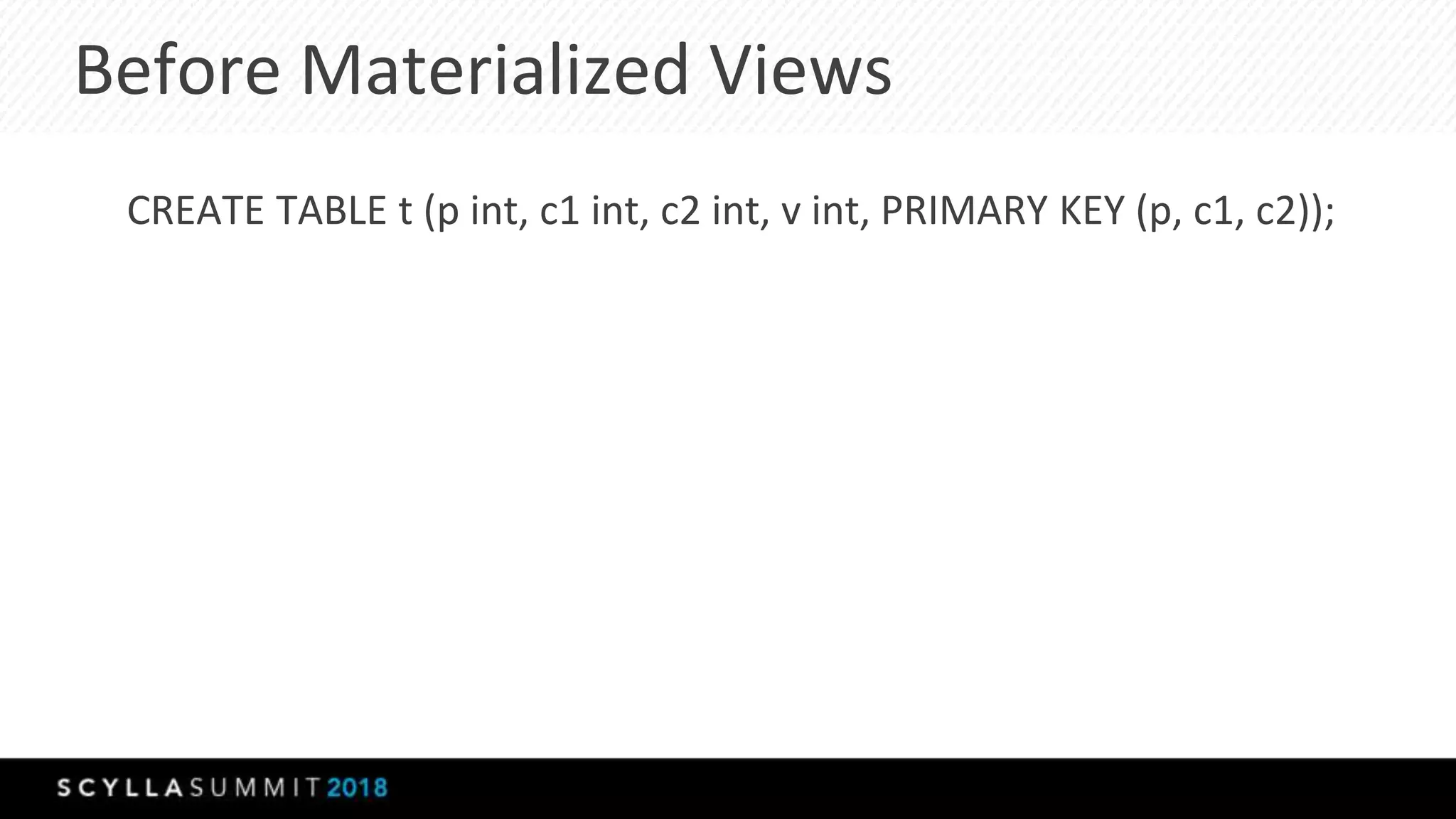
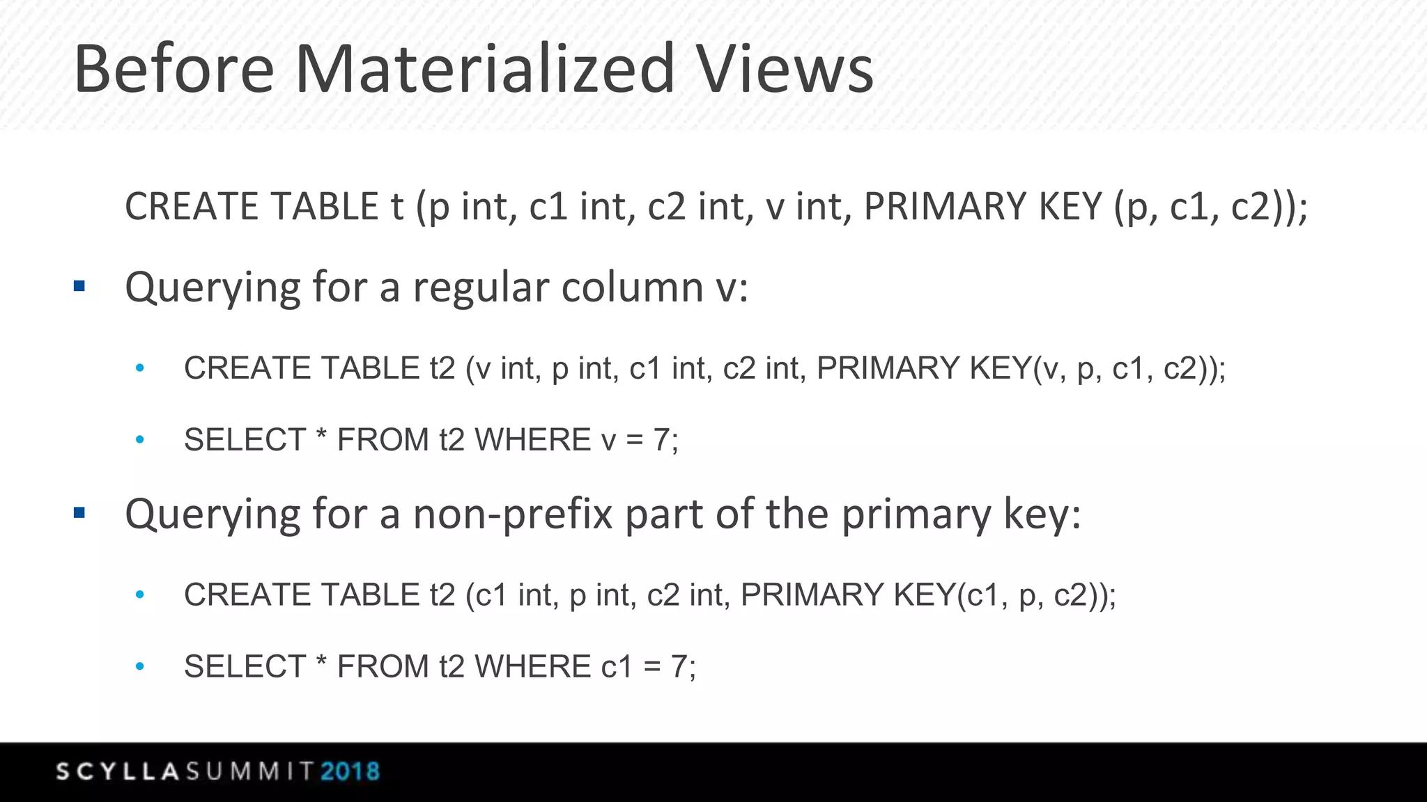
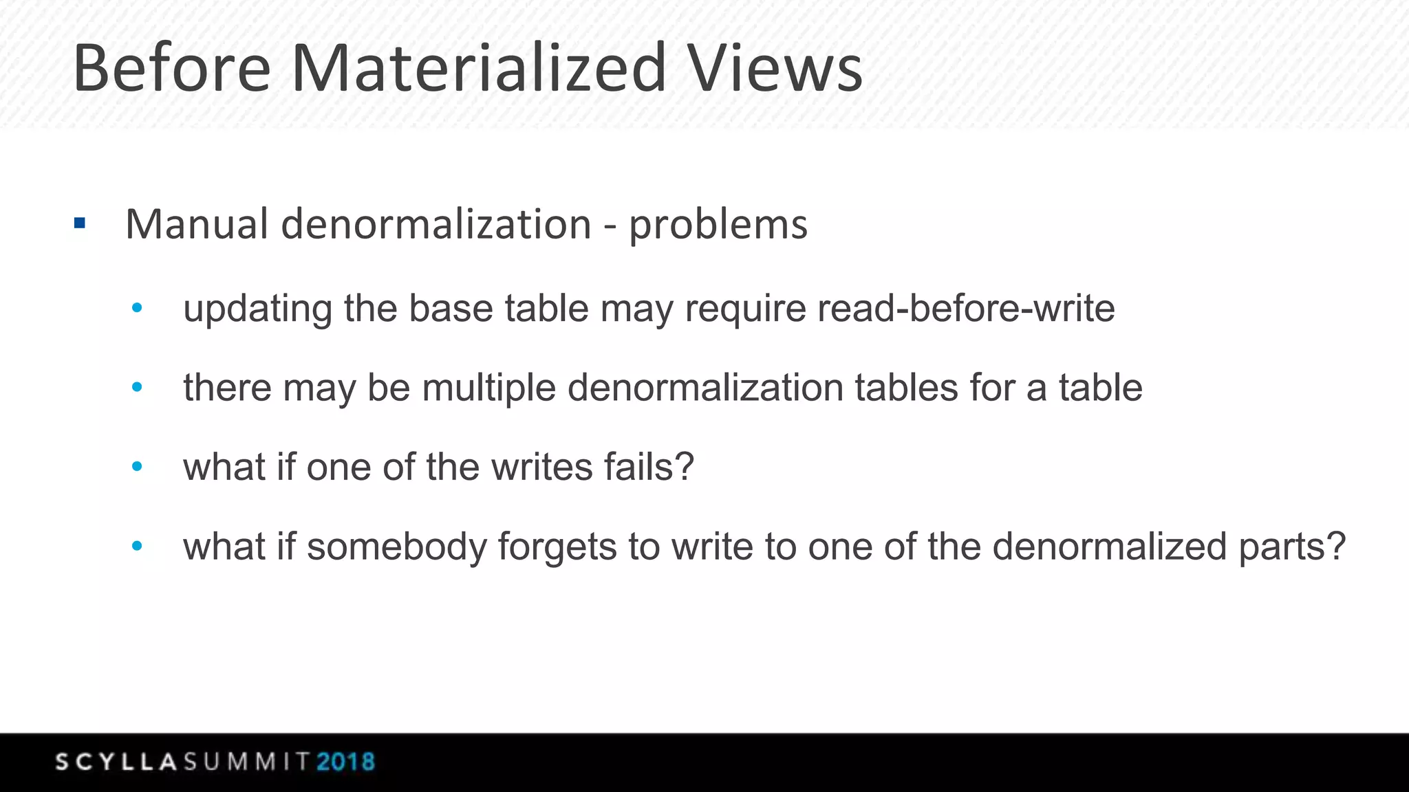
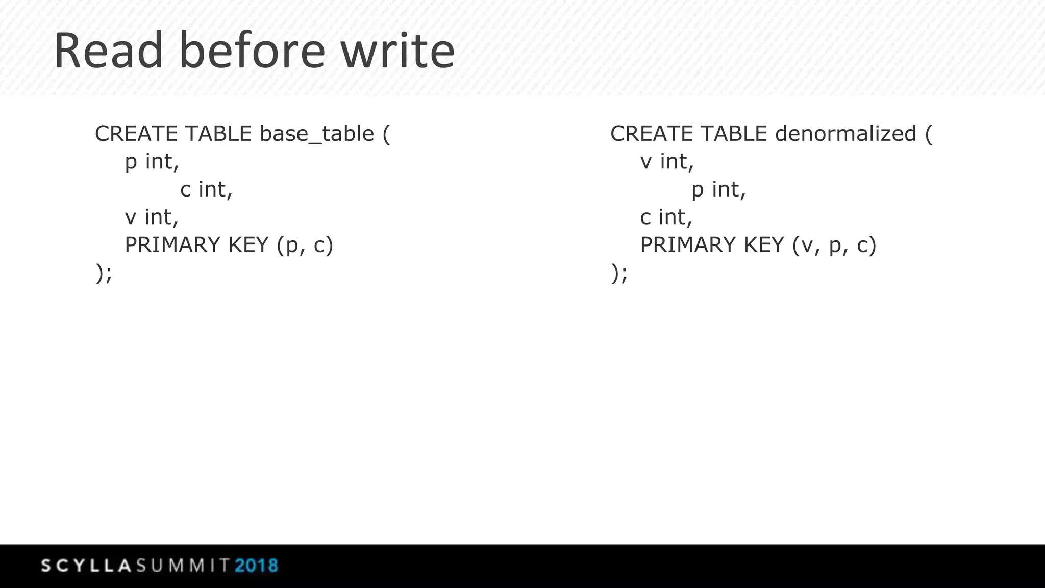
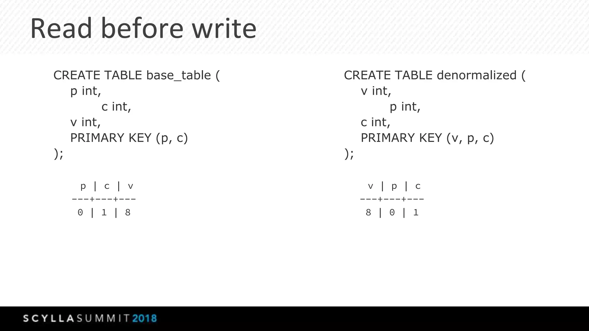
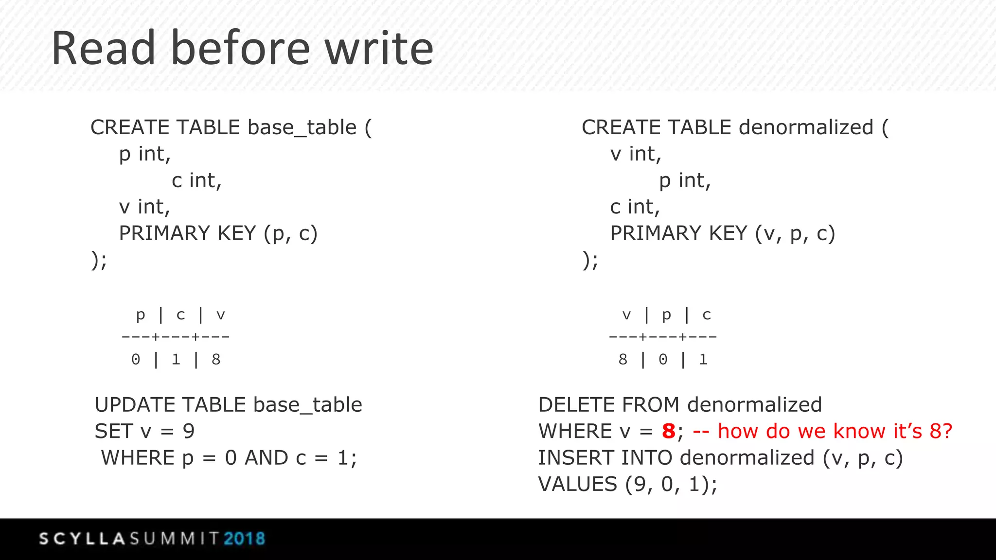
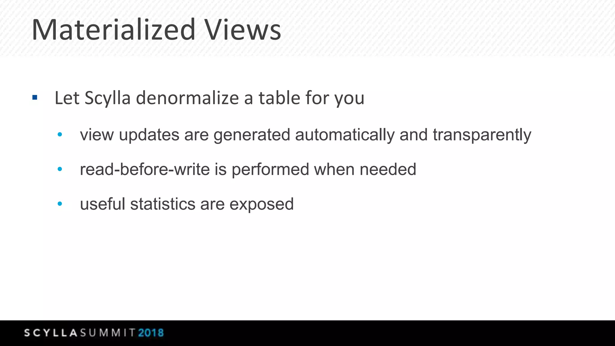
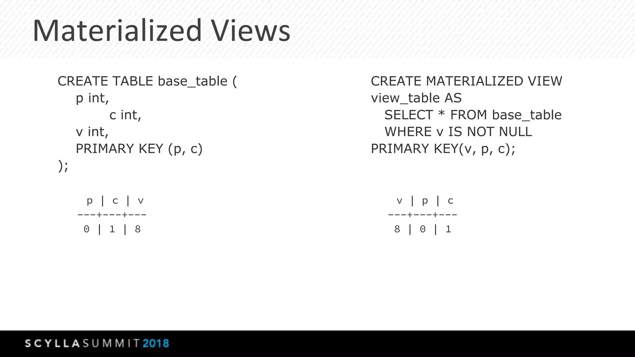
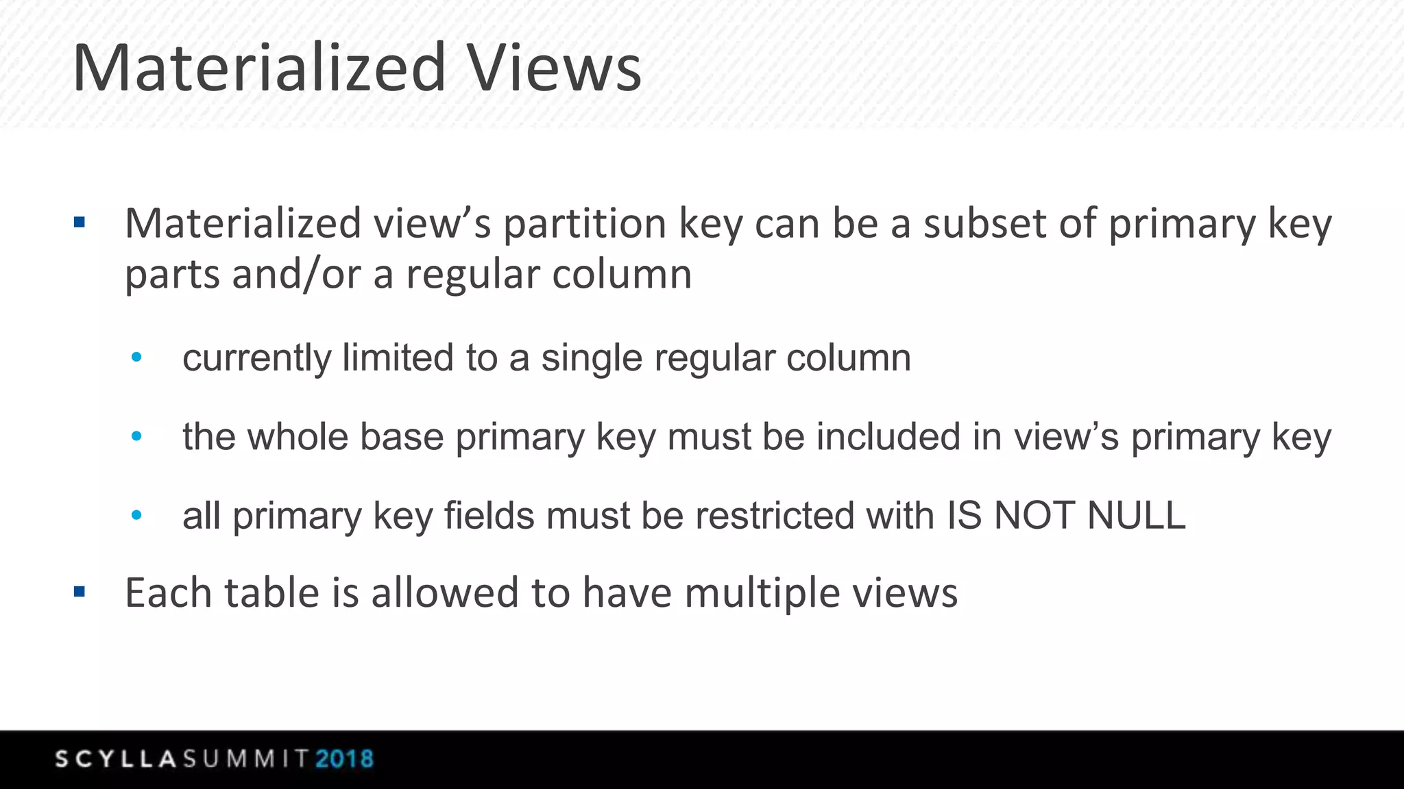
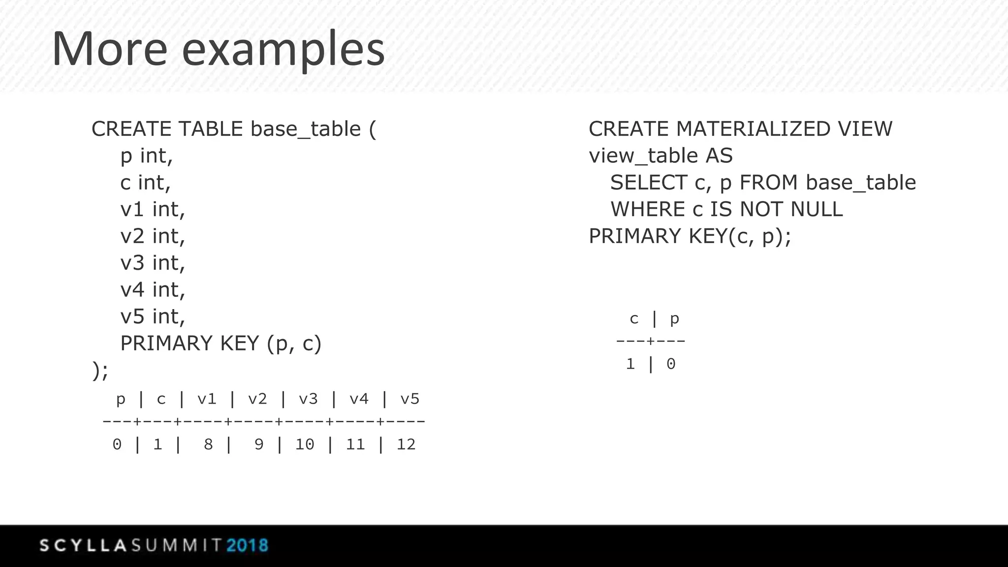
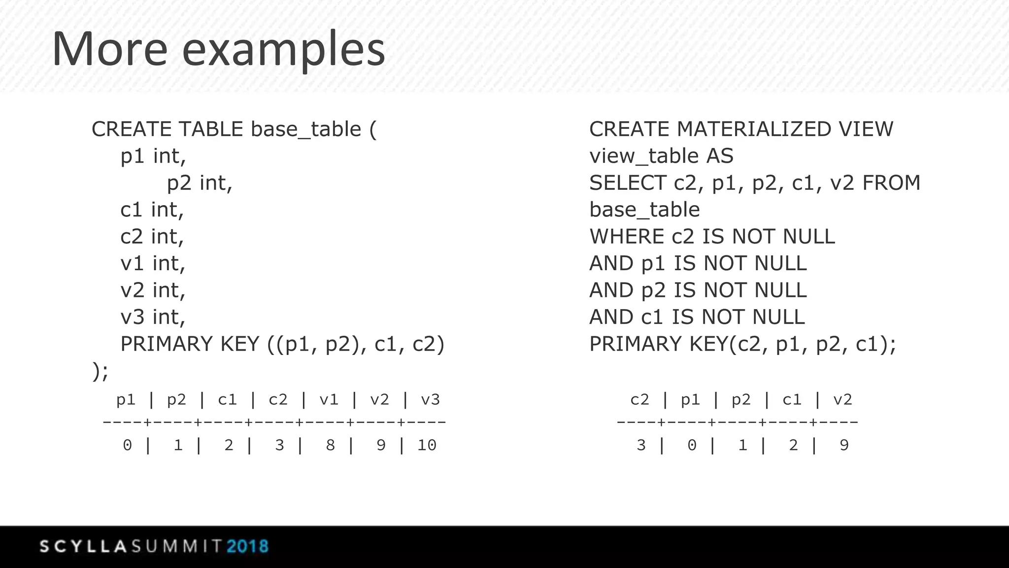
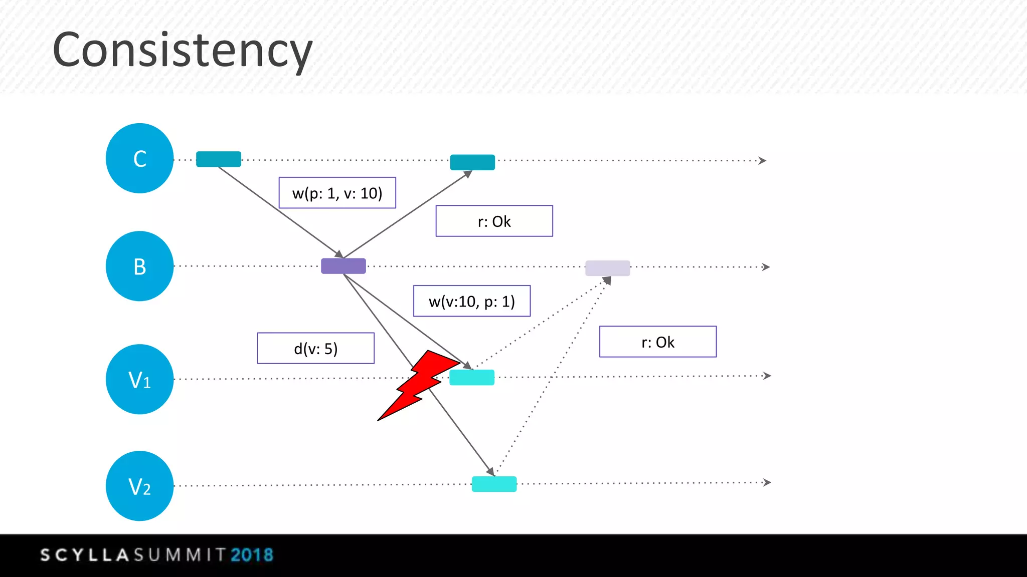
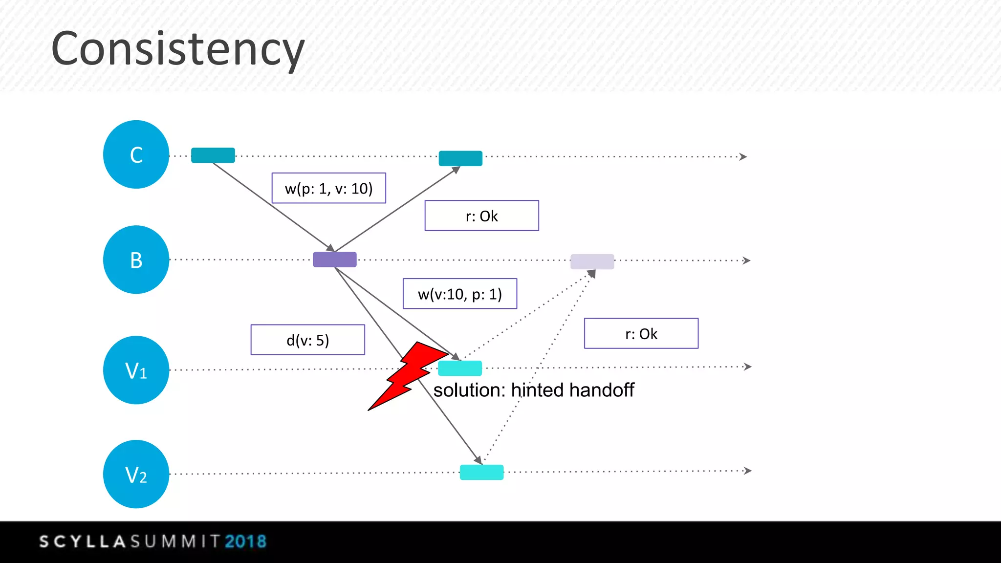
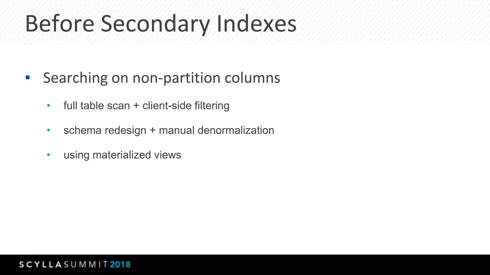
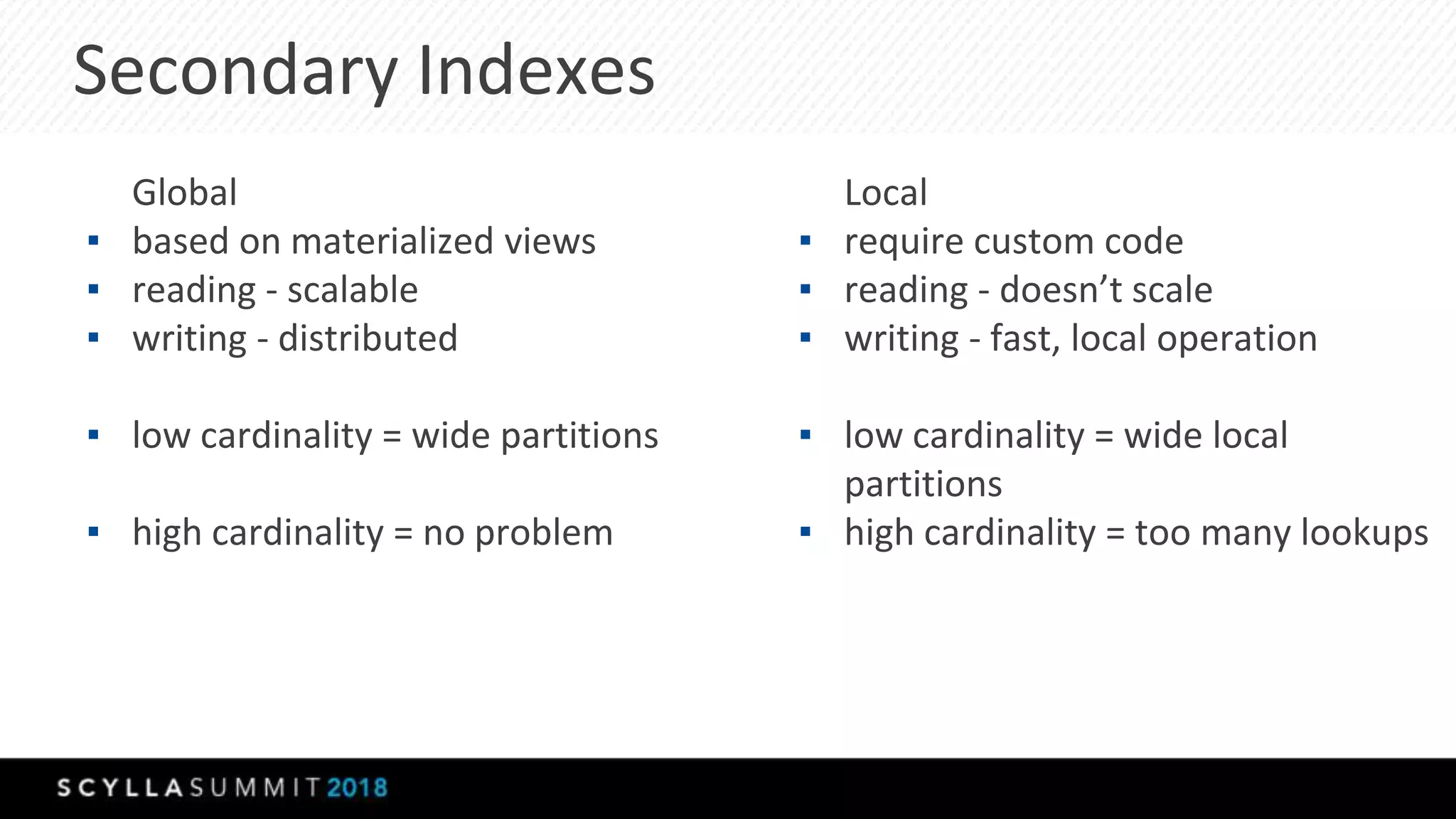
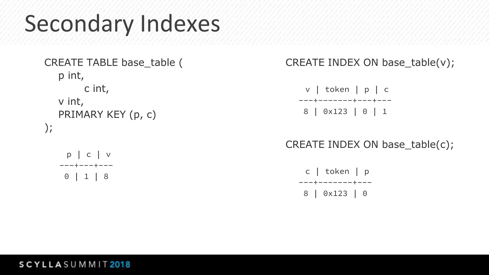
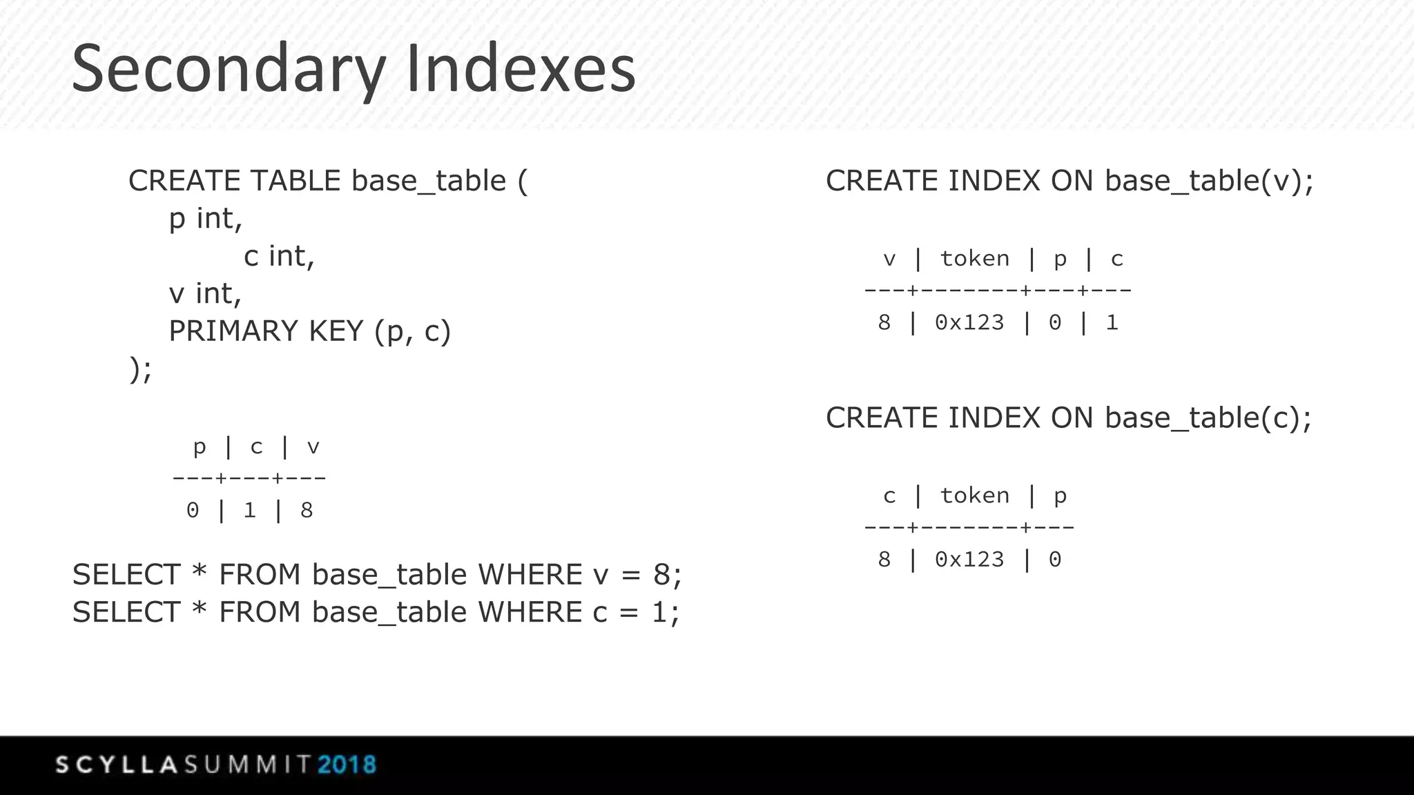
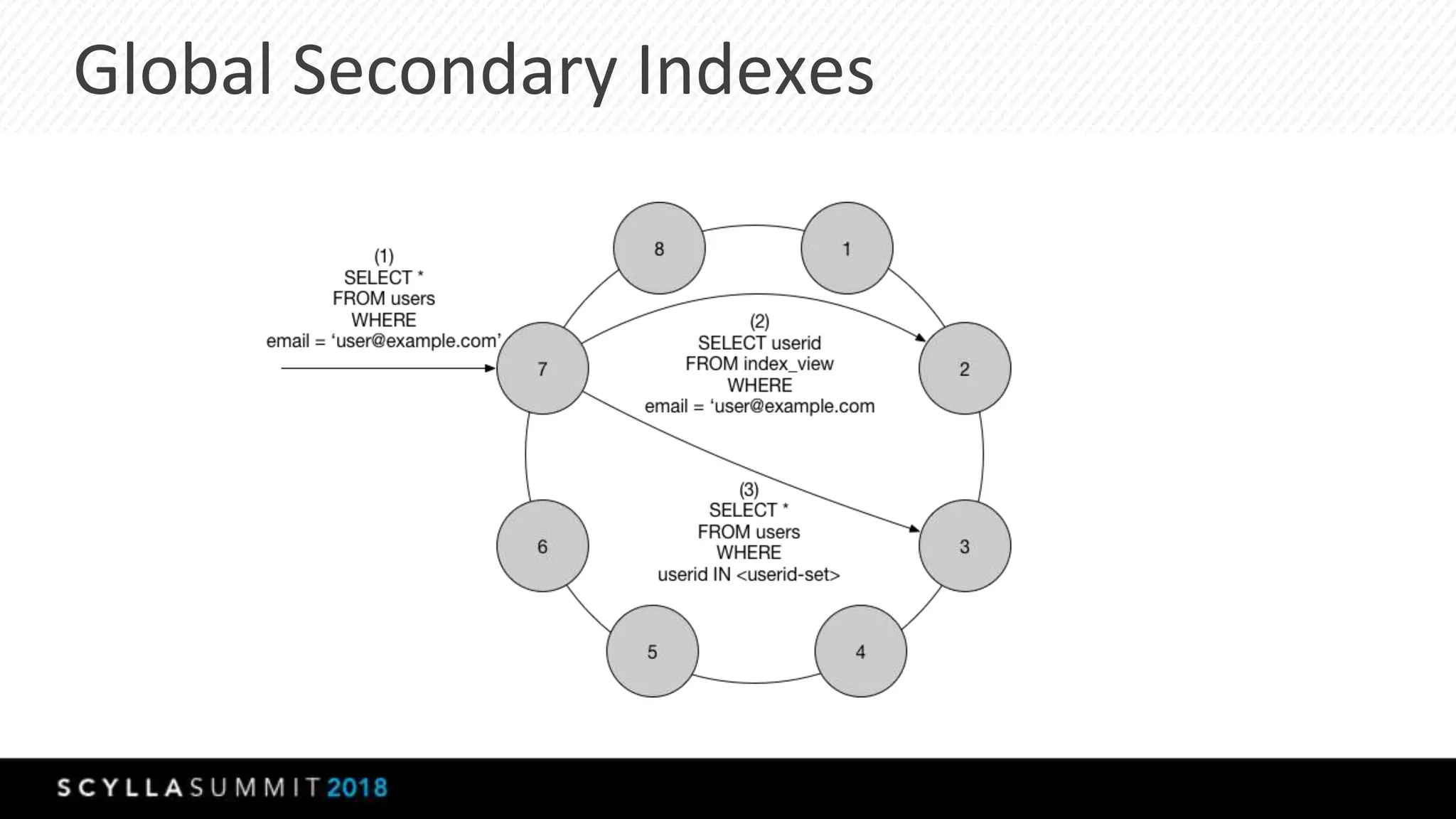
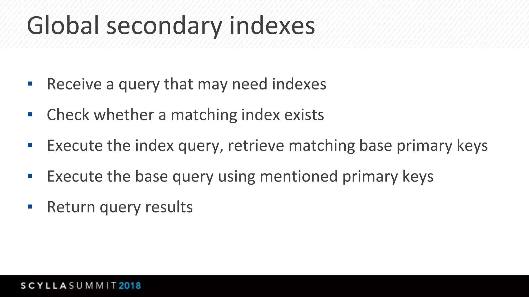
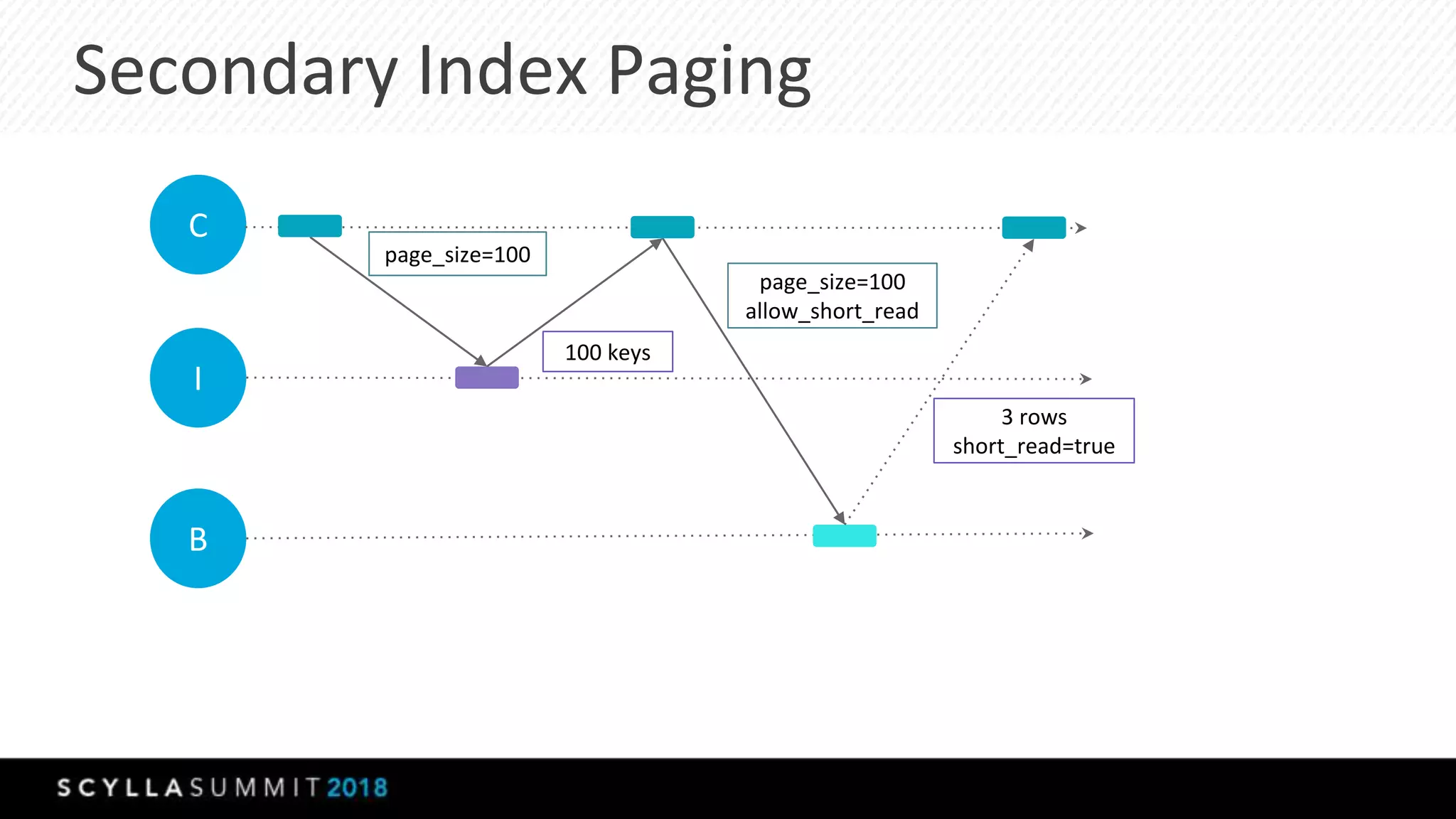
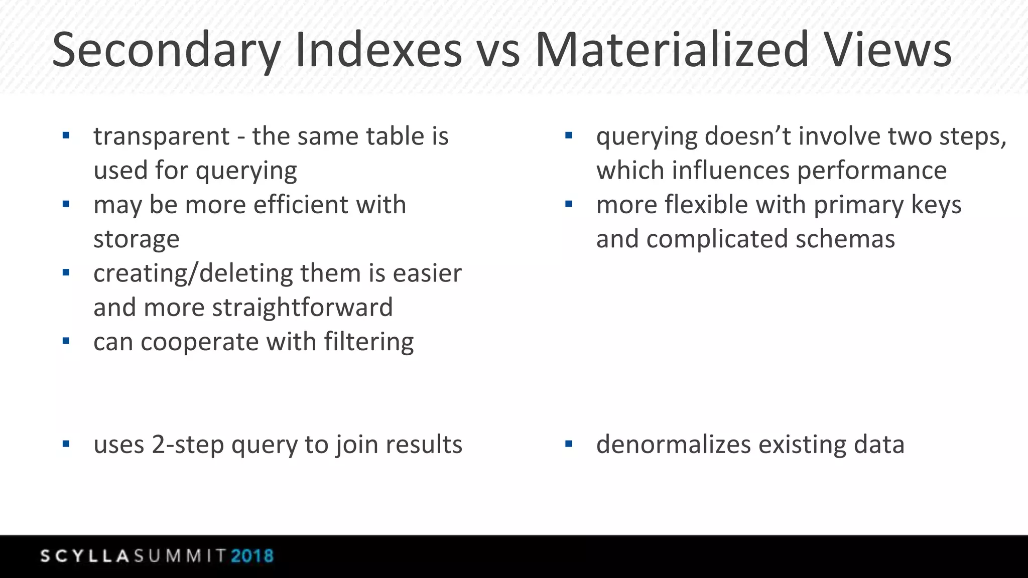
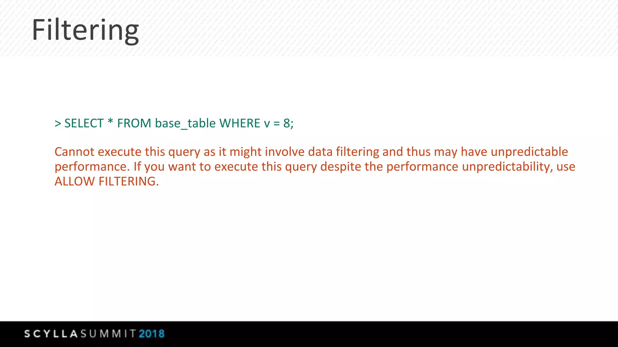
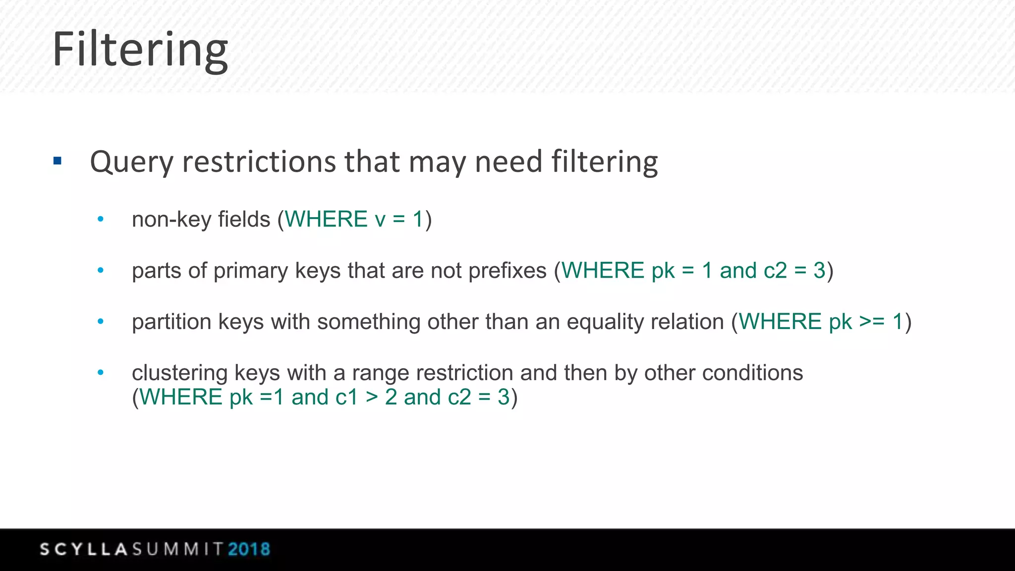
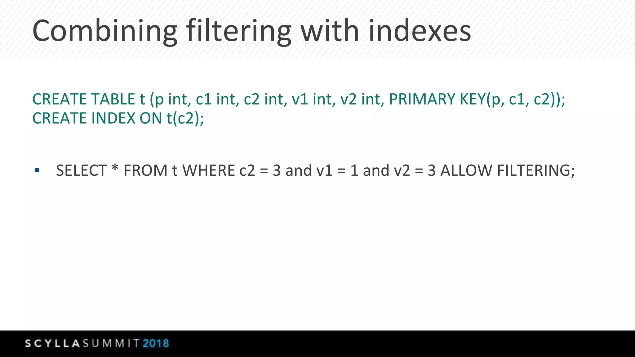
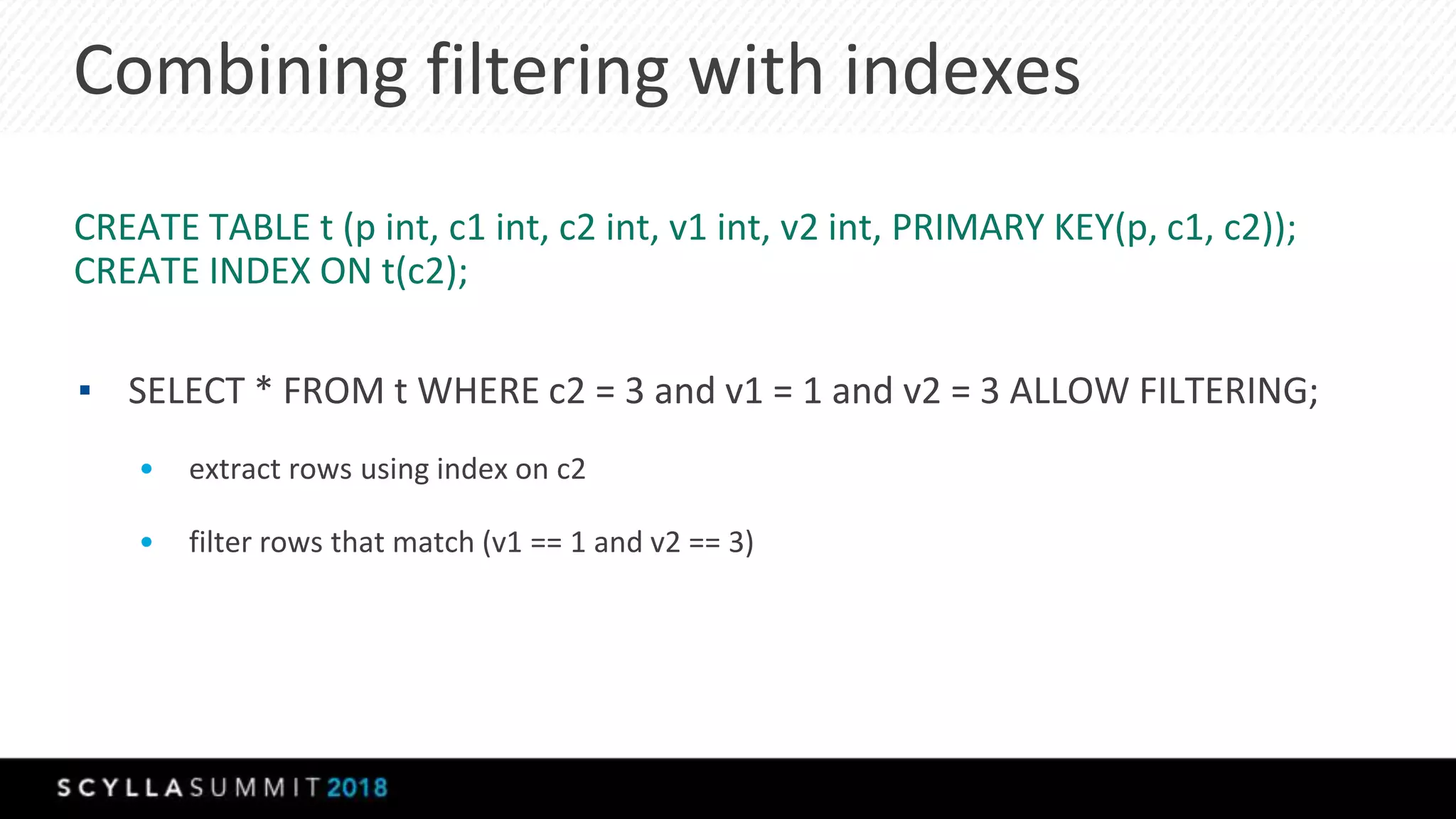
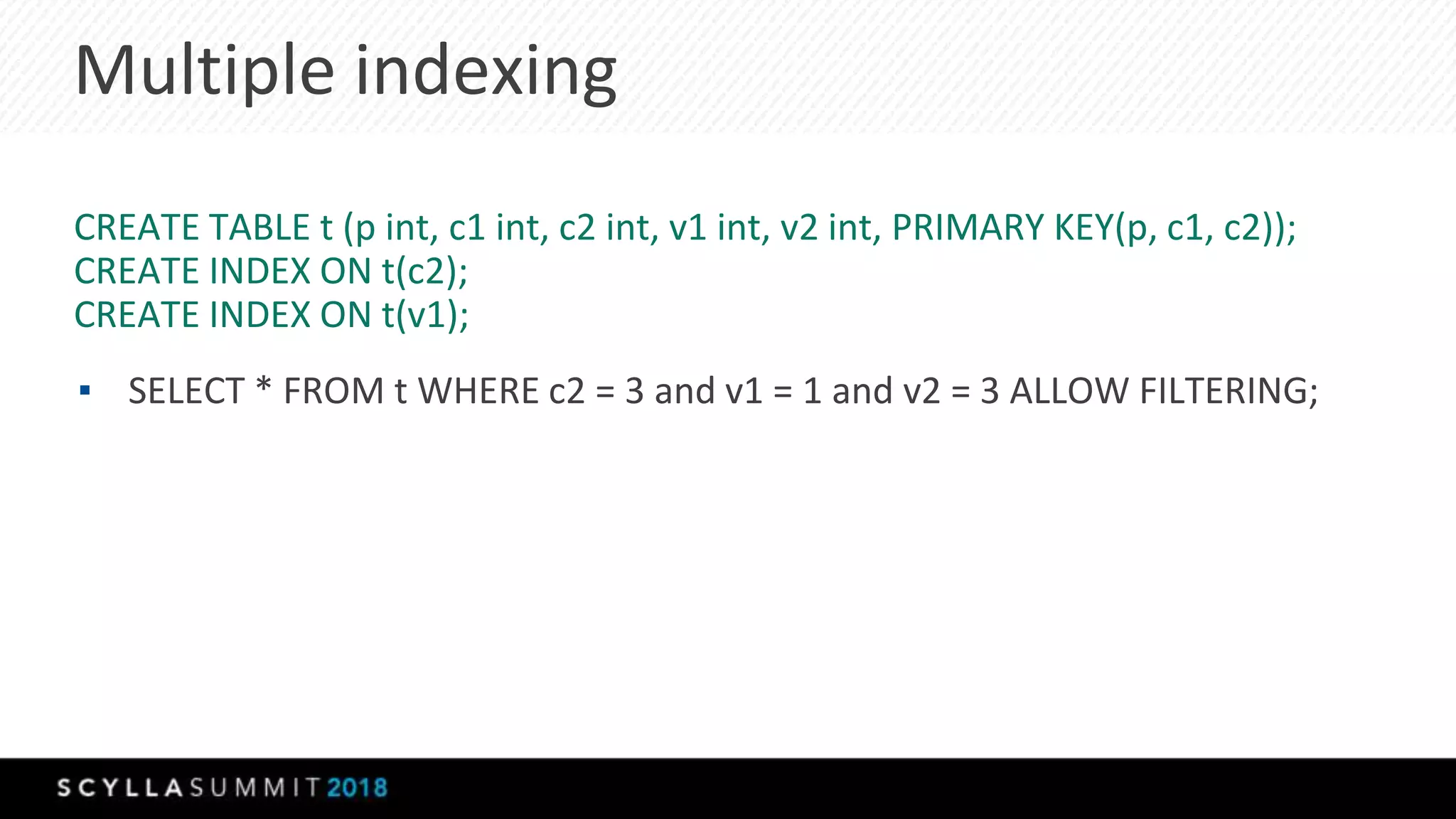
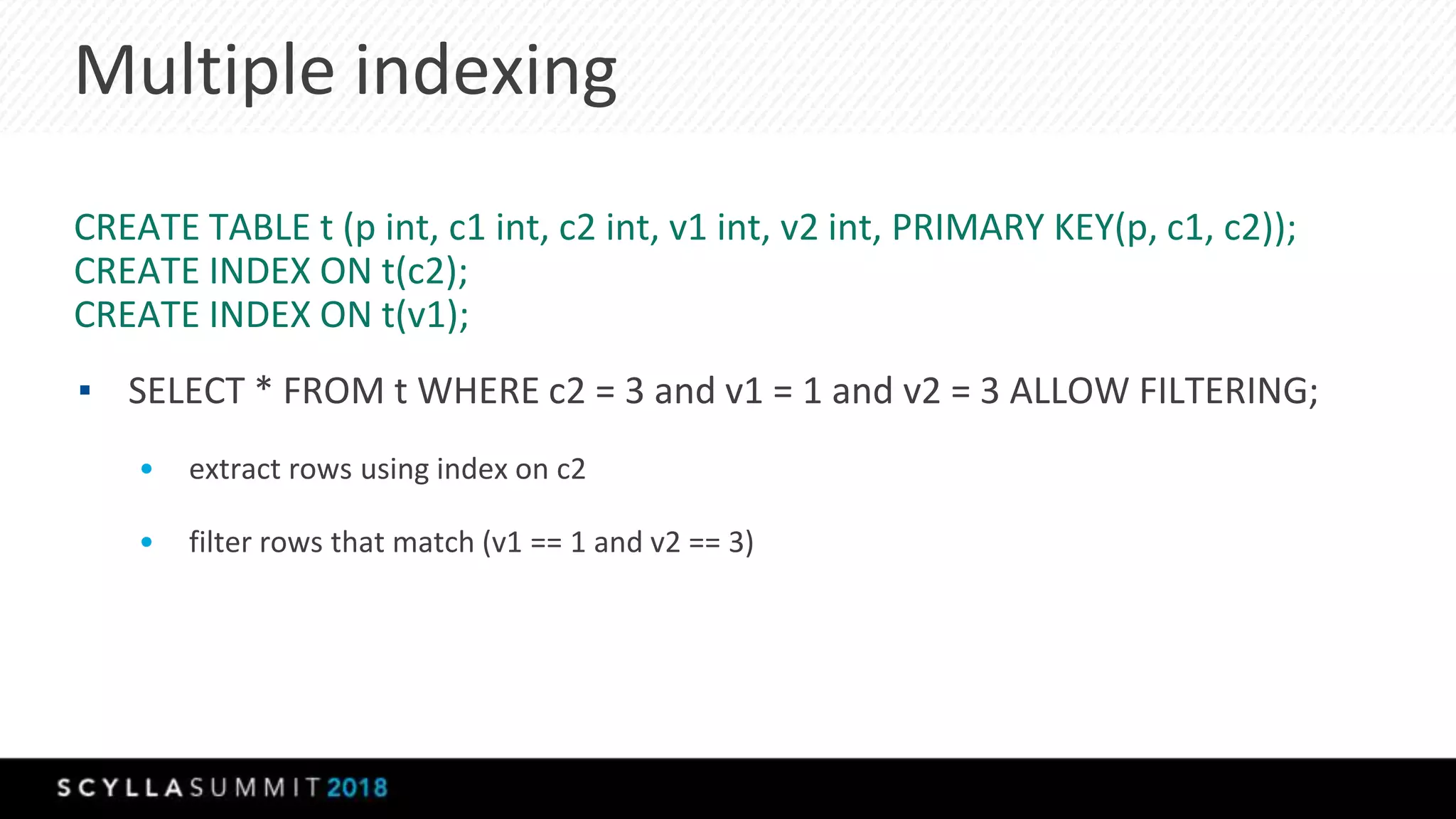
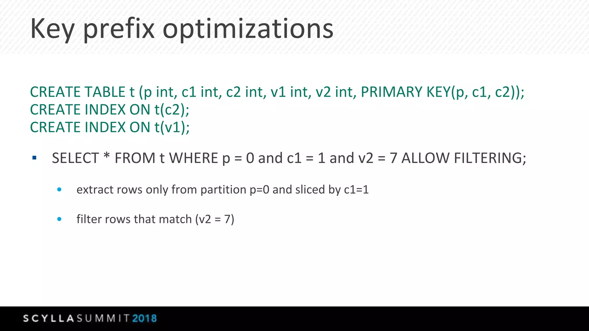
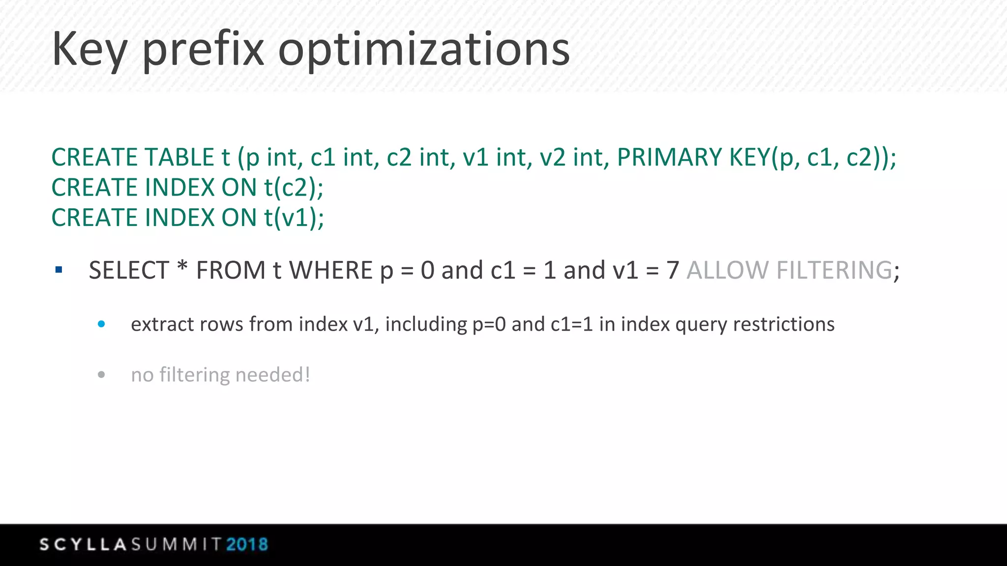
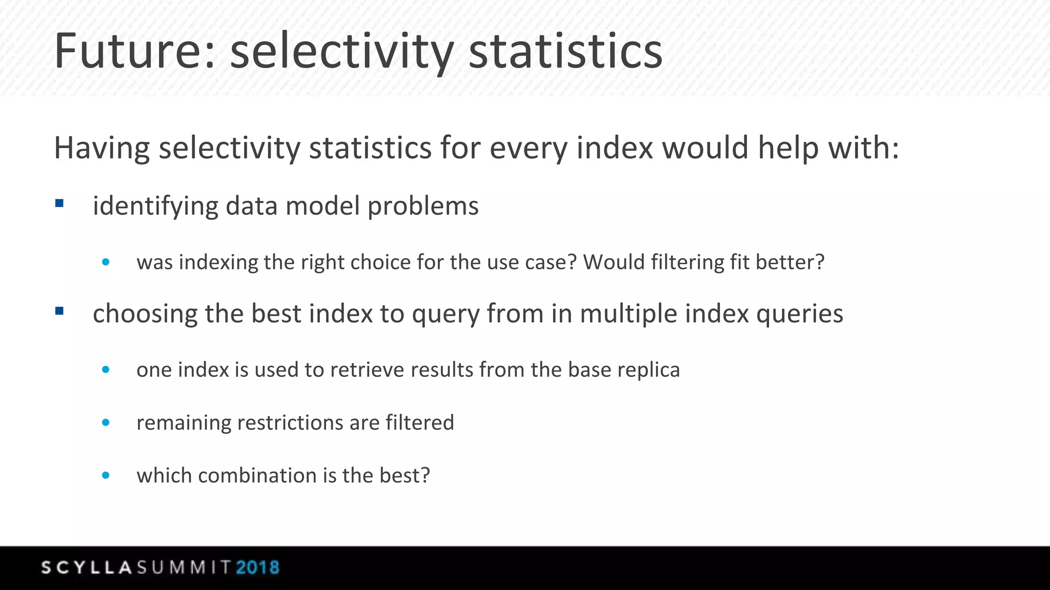
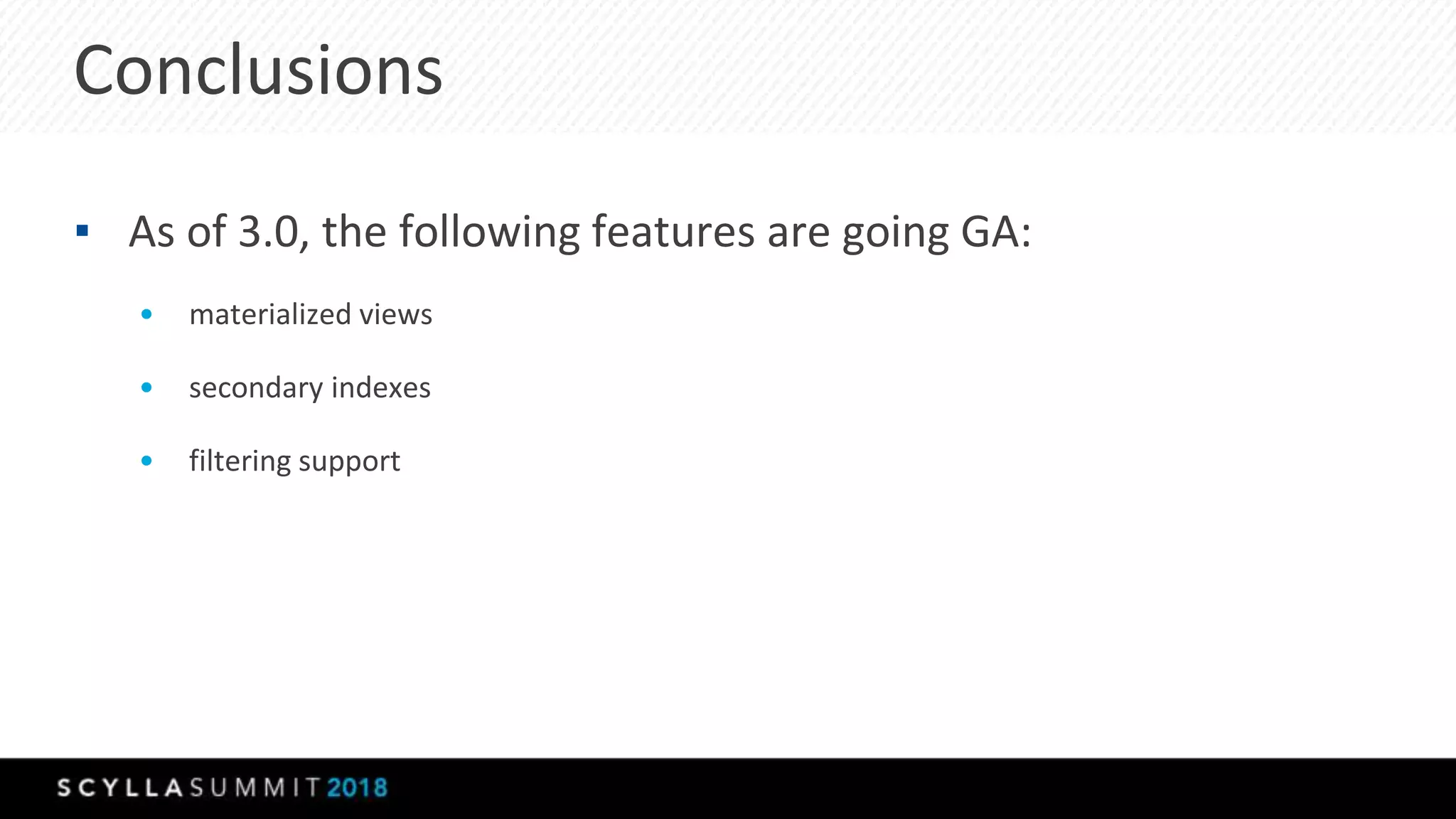
Materialized Views and
Secondary Indexes in Scylla:
They are finally here!
Piotr Sarna
Software Engineer @ScyllaDB
Presenter bio
Piotr is a software engineer very keen on open-source projects
and C++. He previously developed an open-source distributed
file system and had a brief adventure with Linux kernel during
an apprenticeship at Samsung Electronics. Piotr graduated from
University of Warsaw with MSc in Computer Science.
Agenda
▪ Introduction
▪ Materialized Views
▪ Secondary Indexes
▪ Filtering
▪ Summary
Introduction
Why finally?
▪ Materialized views
• experimental in 2.0
▪ Secondary indexes
• experimental in 2.1
▪ Filtering
Why finally?
▪ Materialized views
• experimental in 2.0, production-ready since 3.0
▪ Secondary indexes
• experimental in 2.1, production-ready since 3.0
▪ Filtering
• production-ready since 3.0
Materialized Views
Before Materialized Views
▪ How to query by something else other than primary key
columns?
Before Materialized Views
CREATE TABLE t (p int, c1 int, c2 int, v int, PRIMARY KEY (p, c1, c2));
Before Materialized Views
CREATE TABLE t (p int, c1 int, c2 int, v int, PRIMARY KEY (p, c1, c2));
▪ Querying for a regular column v:
• CREATE TABLE t2 (v int, p int, c1 int, c2 int, PRIMARY KEY(v, p, c1, c2));
• SELECT * FROM t2 WHERE v = 7;
▪ Querying for a non-prefix part of the primary key:
• CREATE TABLE t2 (c1 int, p int, c2 int, PRIMARY KEY(c1, p, c2));
• SELECT * FROM t2 WHERE c1 = 7;
Before Materialized Views
▪ Manual denormalization - problems
• updating the base table may require read-before-write
• there may be multiple denormalization tables for a table
• what if one of the writes fails?
• what if somebody forgets to write to one of the denormalized parts?
Read before write
CREATE TABLE base_table (
p int,
c int,
v int,
PRIMARY KEY (p, c)
);
CREATE TABLE denormalized (
v int,
p int,
c int,
PRIMARY KEY (v, p, c)
);
Read before write
CREATE TABLE base_table (
p int,
c int,
v int,
PRIMARY KEY (p, c)
);
p | c | v
---+---+---
0 | 1 | 8
CREATE TABLE denormalized (
v int,
p int,
c int,
PRIMARY KEY (v, p, c)
);
v | p | c
---+---+---
8 | 0 | 1
Read before write
CREATE TABLE base_table (
p int,
c int,
v int,
PRIMARY KEY (p, c)
);
p | c | v
---+---+---
0 | 1 | 8
UPDATE TABLE base_table
SET v = 9
WHERE p = 0 AND c = 1;
CREATE TABLE denormalized (
v int,
p int,
c int,
PRIMARY KEY (v, p, c)
);
v | p | c
---+---+---
8 | 0 | 1
DELETE FROM denormalized
WHERE v = 8; -- how do we know it’s 8?
INSERT INTO denormalized (v, p, c)
VALUES (9, 0, 1);
Materialized Views
▪ Let Scylla denormalize a table for you
• view updates are generated automatically and transparently
• read-before-write is performed when needed
• useful statistics are exposed
Materialized Views
CREATE TABLE base_table (
p int,
c int,
v int,
PRIMARY KEY (p, c)
);
p | c | v
---+---+---
0 | 1 | 8
CREATE MATERIALIZED VIEW
view_table AS
SELECT * FROM base_table
WHERE v IS NOT NULL
PRIMARY KEY(v, p, c);
v | p | c
---+---+---
8 | 0 | 1
Materialized Views
▪ Materialized view’s partition key can be a subset of primary key
parts and/or a regular column
• currently limited to a single regular column
• the whole base primary key must be included in view’s primary key
• all primary key fields must be restricted with IS NOT NULL
▪ Each table is allowed to have multiple views
More examples
CREATE TABLE base_table (
p int,
c int,
v1 int,
v2 int,
v3 int,
v4 int,
v5 int,
PRIMARY KEY (p, c)
);
p | c | v1 | v2 | v3 | v4 | v5
---+---+----+----+----+----+----
0 | 1 | 8 | 9 | 10 | 11 | 12
CREATE MATERIALIZED VIEW
view_table AS
SELECT c, p FROM base_table
WHERE c IS NOT NULL
PRIMARY KEY(c, p);
c | p
---+---
1 | 0
More examples
CREATE TABLE base_table (
p1 int,
p2 int,
c1 int,
c2 int,
v1 int,
v2 int,
v3 int,
PRIMARY KEY ((p1, p2), c1, c2)
);
p1 | p2 | c1 | c2 | v1 | v2 | v3
----+----+----+----+----+----+----
0 | 1 | 2 | 3 | 8 | 9 | 10
CREATE MATERIALIZED VIEW
view_table AS
SELECT c2, p1, p2, c1, v2 FROM
base_table
WHERE c2 IS NOT NULL
AND p1 IS NOT NULL
AND p2 IS NOT NULL
AND c1 IS NOT NULL
PRIMARY KEY(c2, p1, p2, c1);
c2 | p1 | p2 | c1 | v2
----+----+----+----+----
3 | 0 | 1 | 2 | 9
Challenges
▪ View rows must be eventually consistent with their base counterparts
• all updates should be propagated - inserts, updates, deletes
• updates should not be lost in case of temporary failures/restarts
▪ Cluster must not be overloaded with mv updates - backpressure
• each base write may trigger multiple independent updates
• so can streaming
▪ Views created on an existing table should fill themselves
with existing base data - view building
Consistency - synchronous model
C
B
V1
w(p: 1, v: 10)
V2
d(v: 5)
w(v:10, p: 1)
r: Ok
r: Ok
Consistency - asynchronous model
C
B
V1
w(p: 1, v: 10)
V2
d(v: 5)
w(v:10, p: 1)
r: Ok
r: Ok
Consistency
C
B
V1
w(p: 1, v: 10)
V2
d(v: 5)
w(v:10, p: 1)
r: Ok
r: Ok
Consistency
C
B
V1
w(p: 1, v: 10)
V2
d(v: 5)
w(v:10, p: 1)
r: Ok
r: Ok
Consistency
C
B
V1
w(p: 1, v: 10)
V2
d(v: 5)
w(v:10, p: 1)
r: Ok
r: Ok
solution: hinted handoff
Hinted handoff for materialized views
▪ Failed updates are stored on base node as hints
▪ They will be resent once the paired node is available
View building
▪ Views created on existing tables will be incrementally built from
existing data
▪ Progress can be tracked via system tables:
• system.views_builds_in_progress
• system.built_views
Backpressure
▪ a single user write can trigger multiple mv updates
▪ backpressure prevents overloading the cluster with them
• base replicas report their load to the coordinator
• coordinator is allowed to delay serving new user writes to lower the pressure
▪ there’s a whole presentation about the topic by Nadav Har’El
Public design document: https://docs.google.com/document/d/1J6GeLBvN8_c3SbLVp8YsOXHcLc9nOLlRY7pC6MH3JWo
Streaming
▪ Efficient way of sending data from one node to another
▪ Moves data directly to sstables of the target node,
bypassing the full write path
▪ Used under the hood of several cluster operations, e.g.:
• bootstrap
• repair
• rebuild
▪ In some cases, streamed data should generate materialized view
updates to ensure consistency
• unconditionally during node repair
• when the view is not yet completely built
▪ Affected sstables are stored and used to generate MV updates
Streaming
Secondary Indexes
Before Secondary Indexes
▪ Searching on non-partition columns
• full table scan + client-side filtering
• schema redesign + manual denormalization
• using materialized views
Secondary Indexes
Global
▪ based on materialized views
▪ reading - scalable
▪ writing - distributed
▪ low cardinality = wide partitions
▪ high cardinality = no problem
Local
▪ require custom code
▪ reading - doesn’t scale
▪ writing - fast, local operation
▪ low cardinality = wide local
partitions
▪ high cardinality = too many lookups
Secondary Indexes
CREATE TABLE base_table (
p int,
c int,
v int,
PRIMARY KEY (p, c)
);
p | c | v
---+---+---
0 | 1 | 8
CREATE INDEX ON base_table(v);
v | token | p | c
---+-------+---+---
8 | 0x123 | 0 | 1
CREATE INDEX ON base_table(c);
c | token | p
---+-------+---
8 | 0x123 | 0
Secondary Indexes
CREATE TABLE base_table (
p int,
c int,
v int,
PRIMARY KEY (p, c)
);
p | c | v
---+---+---
0 | 1 | 8
SELECT * FROM base_table WHERE v = 8;
SELECT * FROM base_table WHERE c = 1;
CREATE INDEX ON base_table(v);
v | token | p | c
---+-------+---+---
8 | 0x123 | 0 | 1
CREATE INDEX ON base_table(c);
c | token | p
---+-------+---
8 | 0x123 | 0
Global Secondary Indexes
Global secondary indexes
▪ Receive a query that may need indexes
▪ Check whether a matching index exists
▪ Execute the index query, retrieve matching base primary keys
▪ Execute the base query using mentioned primary keys
▪ Return query results
Secondary index paging
▪ Rows in the index table are small
• only the indexed column, base primary keys and token are stored, all with size limits
• it’s near impossible for 100 index rows to hit the query size limit
▪ Base rows may be much bigger
• even a single row may exceed the query size limit
• not to mention 100 of them
100 rows
page_size=100
100 keys
page_size=100
allow_short_read
Secondary Index Paging
C
I
B
3 rows
short_read=true
page_size=100
100 keys
page_size=100
allow_short_read
Secondary Index Paging
C
I
B
Secondary Indexes vs Materialized Views
▪ transparent - the same table is
used for querying
▪ may be more efficient with
storage
▪ creating/deleting them is easier
and more straightforward
▪ can cooperate with filtering
▪ uses 2-step query to join results
▪ querying doesn’t involve two steps,
which influences performance
▪ more flexible with primary keys
and complicated schemas
▪ denormalizes existing data
Filtering
Filtering
> SELECT * FROM base_table WHERE v = 8;
Cannot execute this query as it might involve data filtering and thus may have unpredictable
performance. If you want to execute this query despite the performance unpredictability, use
ALLOW FILTERING.
Filtering
▪ Query restrictions that may need filtering
• non-key fields (WHERE v = 1)
• parts of primary keys that are not prefixes (WHERE pk = 1 and c2 = 3)
• partition keys with something other than an equality relation (WHERE pk >= 1)
• clustering keys with a range restriction and then by other conditions
(WHERE pk =1 and c1 > 2 and c2 = 3)
Coordinator-side filtering
▪ Coordinator node retrieves all data from nodes
▪ Filtering is applied
▪ Only matching rows are returned to the client
▪ Easily extensible with optimizations (pre-filtering on data nodes
can be implemented and added)
Query selectivity
Low selectivity queries:
▪ return almost all rows (e.g. 70%)
High selectivity queries:
▪ return only a few rows (e.g. 1)
Query selectivity
Low selectivity queries:
▪ return almost all rows (e.g. 70%)
▪ good candidate for filtering
High selectivity queries:
▪ return only a few rows (e.g. 1)
▪ bad candidate for filtering
Filtering alternatives
▪ Materialized views and their alternatives
▪ Secondary indexes and their alternatives
Filtering + indexes
Combining filtering with indexes
CREATE TABLE t (p int, c1 int, c2 int, v1 int, v2 int, PRIMARY KEY(p, c1, c2));
CREATE INDEX ON t(c2);
▪ SELECT * FROM t WHERE c2 = 3 and v1 = 1 and v2 = 3 ALLOW FILTERING;
Combining filtering with indexes
CREATE TABLE t (p int, c1 int, c2 int, v1 int, v2 int, PRIMARY KEY(p, c1, c2));
CREATE INDEX ON t(c2);
▪ SELECT * FROM t WHERE c2 = 3 and v1 = 1 and v2 = 3 ALLOW FILTERING;
• extract rows using index on c2
• filter rows that match (v1 == 1 and v2 == 3)
Multiple indexing
CREATE TABLE t (p int, c1 int, c2 int, v1 int, v2 int, PRIMARY KEY(p, c1, c2));
CREATE INDEX ON t(c2);
CREATE INDEX ON t(v1);
▪ SELECT * FROM t WHERE c2 = 3 and v1 = 1 and v2 = 3 ALLOW FILTERING;
Multiple indexing
CREATE TABLE t (p int, c1 int, c2 int, v1 int, v2 int, PRIMARY KEY(p, c1, c2));
CREATE INDEX ON t(c2);
CREATE INDEX ON t(v1);
▪ SELECT * FROM t WHERE c2 = 3 and v1 = 1 and v2 = 3 ALLOW FILTERING;
• extract rows using index on c2
• filter rows that match (v1 == 1 and v2 == 3)
Key prefix optimizations
CREATE TABLE t (p int, c1 int, c2 int, v1 int, v2 int, PRIMARY KEY(p, c1, c2));
CREATE INDEX ON t(c2);
CREATE INDEX ON t(v1);
▪ SELECT * FROM t WHERE p = 0 and c1 = 1 and v2 = 7 ALLOW FILTERING;
• extract rows only from partition p=0 and sliced by c1=1
• filter rows that match (v2 = 7)
Key prefix optimizations
CREATE TABLE t (p int, c1 int, c2 int, v1 int, v2 int, PRIMARY KEY(p, c1, c2));
CREATE INDEX ON t(c2);
CREATE INDEX ON t(v1);
▪ SELECT * FROM t WHERE p = 0 and c1 = 1 and v1 = 7 ALLOW FILTERING;
• extract rows from index v1, including p=0 and c1=1 in index query restrictions
• no filtering needed!
Future: selectivity statistics
Having selectivity statistics for every index would help with:
▪ identifying data model problems
• was indexing the right choice for the use case? Would filtering fit better?
▪ choosing the best index to query from in multiple index queries
• one index is used to retrieve results from the base replica
• remaining restrictions are filtered
• which combination is the best?
Conclusions
Conclusions
▪ As of 3.0, the following features are going GA:
• materialized views
• secondary indexes
• filtering support
Future plans
▪ MV repair
▪ optimized multi-index support
▪ add replica-side filtering optimizations
▪ as always - optimize even further
Thank You
Any Questions?
Please stay in touch
sarna@scylladb.com

Materialized Views and Secondary Indexes in Scylla: They Are finally here!

  • 1.
    Materialized Views and SecondaryIndexes in Scylla: They are finally here! Piotr Sarna Software Engineer @ScyllaDB
  • 2.
    Presenter bio Piotr isa software engineer very keen on open-source projects and C++. He previously developed an open-source distributed file system and had a brief adventure with Linux kernel during an apprenticeship at Samsung Electronics. Piotr graduated from University of Warsaw with MSc in Computer Science.
  • 3.
    Agenda ▪ Introduction ▪ MaterializedViews ▪ Secondary Indexes ▪ Filtering ▪ Summary
  • 4.
  • 5.
    Why finally? ▪ Materializedviews • experimental in 2.0 ▪ Secondary indexes • experimental in 2.1 ▪ Filtering
  • 6.
    Why finally? ▪ Materializedviews • experimental in 2.0, production-ready since 3.0 ▪ Secondary indexes • experimental in 2.1, production-ready since 3.0 ▪ Filtering • production-ready since 3.0
  • 7.
  • 8.
    Before Materialized Views ▪How to query by something else other than primary key columns?
  • 9.
    Before Materialized Views CREATETABLE t (p int, c1 int, c2 int, v int, PRIMARY KEY (p, c1, c2));
  • 10.
    Before Materialized Views CREATETABLE t (p int, c1 int, c2 int, v int, PRIMARY KEY (p, c1, c2)); ▪ Querying for a regular column v: • CREATE TABLE t2 (v int, p int, c1 int, c2 int, PRIMARY KEY(v, p, c1, c2)); • SELECT * FROM t2 WHERE v = 7; ▪ Querying for a non-prefix part of the primary key: • CREATE TABLE t2 (c1 int, p int, c2 int, PRIMARY KEY(c1, p, c2)); • SELECT * FROM t2 WHERE c1 = 7;
  • 11.
    Before Materialized Views ▪Manual denormalization - problems • updating the base table may require read-before-write • there may be multiple denormalization tables for a table • what if one of the writes fails? • what if somebody forgets to write to one of the denormalized parts?
  • 12.
    Read before write CREATETABLE base_table ( p int, c int, v int, PRIMARY KEY (p, c) ); CREATE TABLE denormalized ( v int, p int, c int, PRIMARY KEY (v, p, c) );
  • 13.
    Read before write CREATETABLE base_table ( p int, c int, v int, PRIMARY KEY (p, c) ); p | c | v ---+---+--- 0 | 1 | 8 CREATE TABLE denormalized ( v int, p int, c int, PRIMARY KEY (v, p, c) ); v | p | c ---+---+--- 8 | 0 | 1
  • 14.
    Read before write CREATETABLE base_table ( p int, c int, v int, PRIMARY KEY (p, c) ); p | c | v ---+---+--- 0 | 1 | 8 UPDATE TABLE base_table SET v = 9 WHERE p = 0 AND c = 1; CREATE TABLE denormalized ( v int, p int, c int, PRIMARY KEY (v, p, c) ); v | p | c ---+---+--- 8 | 0 | 1 DELETE FROM denormalized WHERE v = 8; -- how do we know it’s 8? INSERT INTO denormalized (v, p, c) VALUES (9, 0, 1);
  • 15.
    Materialized Views ▪ LetScylla denormalize a table for you • view updates are generated automatically and transparently • read-before-write is performed when needed • useful statistics are exposed
  • 16.
    Materialized Views CREATE TABLEbase_table ( p int, c int, v int, PRIMARY KEY (p, c) ); p | c | v ---+---+--- 0 | 1 | 8 CREATE MATERIALIZED VIEW view_table AS SELECT * FROM base_table WHERE v IS NOT NULL PRIMARY KEY(v, p, c); v | p | c ---+---+--- 8 | 0 | 1
  • 17.
    Materialized Views ▪ Materializedview’s partition key can be a subset of primary key parts and/or a regular column • currently limited to a single regular column • the whole base primary key must be included in view’s primary key • all primary key fields must be restricted with IS NOT NULL ▪ Each table is allowed to have multiple views
  • 18.
    More examples CREATE TABLEbase_table ( p int, c int, v1 int, v2 int, v3 int, v4 int, v5 int, PRIMARY KEY (p, c) ); p | c | v1 | v2 | v3 | v4 | v5 ---+---+----+----+----+----+---- 0 | 1 | 8 | 9 | 10 | 11 | 12 CREATE MATERIALIZED VIEW view_table AS SELECT c, p FROM base_table WHERE c IS NOT NULL PRIMARY KEY(c, p); c | p ---+--- 1 | 0
  • 19.
    More examples CREATE TABLEbase_table ( p1 int, p2 int, c1 int, c2 int, v1 int, v2 int, v3 int, PRIMARY KEY ((p1, p2), c1, c2) ); p1 | p2 | c1 | c2 | v1 | v2 | v3 ----+----+----+----+----+----+---- 0 | 1 | 2 | 3 | 8 | 9 | 10 CREATE MATERIALIZED VIEW view_table AS SELECT c2, p1, p2, c1, v2 FROM base_table WHERE c2 IS NOT NULL AND p1 IS NOT NULL AND p2 IS NOT NULL AND c1 IS NOT NULL PRIMARY KEY(c2, p1, p2, c1); c2 | p1 | p2 | c1 | v2 ----+----+----+----+---- 3 | 0 | 1 | 2 | 9
  • 20.
    Challenges ▪ View rowsmust be eventually consistent with their base counterparts • all updates should be propagated - inserts, updates, deletes • updates should not be lost in case of temporary failures/restarts ▪ Cluster must not be overloaded with mv updates - backpressure • each base write may trigger multiple independent updates • so can streaming ▪ Views created on an existing table should fill themselves with existing base data - view building
  • 21.
    Consistency - synchronousmodel C B V1 w(p: 1, v: 10) V2 d(v: 5) w(v:10, p: 1) r: Ok r: Ok
  • 22.
    Consistency - asynchronousmodel C B V1 w(p: 1, v: 10) V2 d(v: 5) w(v:10, p: 1) r: Ok r: Ok
  • 23.
    Consistency C B V1 w(p: 1, v:10) V2 d(v: 5) w(v:10, p: 1) r: Ok r: Ok
  • 24.
    Consistency C B V1 w(p: 1, v:10) V2 d(v: 5) w(v:10, p: 1) r: Ok r: Ok
  • 25.
    Consistency C B V1 w(p: 1, v:10) V2 d(v: 5) w(v:10, p: 1) r: Ok r: Ok solution: hinted handoff
  • 26.
    Hinted handoff formaterialized views ▪ Failed updates are stored on base node as hints ▪ They will be resent once the paired node is available
  • 27.
    View building ▪ Viewscreated on existing tables will be incrementally built from existing data ▪ Progress can be tracked via system tables: • system.views_builds_in_progress • system.built_views
  • 28.
    Backpressure ▪ a singleuser write can trigger multiple mv updates ▪ backpressure prevents overloading the cluster with them • base replicas report their load to the coordinator • coordinator is allowed to delay serving new user writes to lower the pressure ▪ there’s a whole presentation about the topic by Nadav Har’El Public design document: https://docs.google.com/document/d/1J6GeLBvN8_c3SbLVp8YsOXHcLc9nOLlRY7pC6MH3JWo
  • 29.
    Streaming ▪ Efficient wayof sending data from one node to another ▪ Moves data directly to sstables of the target node, bypassing the full write path ▪ Used under the hood of several cluster operations, e.g.: • bootstrap • repair • rebuild
  • 30.
    ▪ In somecases, streamed data should generate materialized view updates to ensure consistency • unconditionally during node repair • when the view is not yet completely built ▪ Affected sstables are stored and used to generate MV updates Streaming
  • 31.
  • 32.
    Before Secondary Indexes ▪Searching on non-partition columns • full table scan + client-side filtering • schema redesign + manual denormalization • using materialized views
  • 33.
    Secondary Indexes Global ▪ basedon materialized views ▪ reading - scalable ▪ writing - distributed ▪ low cardinality = wide partitions ▪ high cardinality = no problem Local ▪ require custom code ▪ reading - doesn’t scale ▪ writing - fast, local operation ▪ low cardinality = wide local partitions ▪ high cardinality = too many lookups
  • 34.
    Secondary Indexes CREATE TABLEbase_table ( p int, c int, v int, PRIMARY KEY (p, c) ); p | c | v ---+---+--- 0 | 1 | 8 CREATE INDEX ON base_table(v); v | token | p | c ---+-------+---+--- 8 | 0x123 | 0 | 1 CREATE INDEX ON base_table(c); c | token | p ---+-------+--- 8 | 0x123 | 0
  • 35.
    Secondary Indexes CREATE TABLEbase_table ( p int, c int, v int, PRIMARY KEY (p, c) ); p | c | v ---+---+--- 0 | 1 | 8 SELECT * FROM base_table WHERE v = 8; SELECT * FROM base_table WHERE c = 1; CREATE INDEX ON base_table(v); v | token | p | c ---+-------+---+--- 8 | 0x123 | 0 | 1 CREATE INDEX ON base_table(c); c | token | p ---+-------+--- 8 | 0x123 | 0
  • 36.
  • 37.
    Global secondary indexes ▪Receive a query that may need indexes ▪ Check whether a matching index exists ▪ Execute the index query, retrieve matching base primary keys ▪ Execute the base query using mentioned primary keys ▪ Return query results
  • 38.
    Secondary index paging ▪Rows in the index table are small • only the indexed column, base primary keys and token are stored, all with size limits • it’s near impossible for 100 index rows to hit the query size limit ▪ Base rows may be much bigger • even a single row may exceed the query size limit • not to mention 100 of them
  • 39.
  • 40.
  • 41.
    Secondary Indexes vsMaterialized Views ▪ transparent - the same table is used for querying ▪ may be more efficient with storage ▪ creating/deleting them is easier and more straightforward ▪ can cooperate with filtering ▪ uses 2-step query to join results ▪ querying doesn’t involve two steps, which influences performance ▪ more flexible with primary keys and complicated schemas ▪ denormalizes existing data
  • 42.
  • 43.
    Filtering > SELECT *FROM base_table WHERE v = 8; Cannot execute this query as it might involve data filtering and thus may have unpredictable performance. If you want to execute this query despite the performance unpredictability, use ALLOW FILTERING.
  • 44.
    Filtering ▪ Query restrictionsthat may need filtering • non-key fields (WHERE v = 1) • parts of primary keys that are not prefixes (WHERE pk = 1 and c2 = 3) • partition keys with something other than an equality relation (WHERE pk >= 1) • clustering keys with a range restriction and then by other conditions (WHERE pk =1 and c1 > 2 and c2 = 3)
  • 45.
    Coordinator-side filtering ▪ Coordinatornode retrieves all data from nodes ▪ Filtering is applied ▪ Only matching rows are returned to the client ▪ Easily extensible with optimizations (pre-filtering on data nodes can be implemented and added)
  • 46.
    Query selectivity Low selectivityqueries: ▪ return almost all rows (e.g. 70%) High selectivity queries: ▪ return only a few rows (e.g. 1)
  • 47.
    Query selectivity Low selectivityqueries: ▪ return almost all rows (e.g. 70%) ▪ good candidate for filtering High selectivity queries: ▪ return only a few rows (e.g. 1) ▪ bad candidate for filtering
  • 48.
    Filtering alternatives ▪ Materializedviews and their alternatives ▪ Secondary indexes and their alternatives
  • 49.
  • 50.
    Combining filtering withindexes CREATE TABLE t (p int, c1 int, c2 int, v1 int, v2 int, PRIMARY KEY(p, c1, c2)); CREATE INDEX ON t(c2); ▪ SELECT * FROM t WHERE c2 = 3 and v1 = 1 and v2 = 3 ALLOW FILTERING;
  • 51.
    Combining filtering withindexes CREATE TABLE t (p int, c1 int, c2 int, v1 int, v2 int, PRIMARY KEY(p, c1, c2)); CREATE INDEX ON t(c2); ▪ SELECT * FROM t WHERE c2 = 3 and v1 = 1 and v2 = 3 ALLOW FILTERING; • extract rows using index on c2 • filter rows that match (v1 == 1 and v2 == 3)
  • 52.
    Multiple indexing CREATE TABLEt (p int, c1 int, c2 int, v1 int, v2 int, PRIMARY KEY(p, c1, c2)); CREATE INDEX ON t(c2); CREATE INDEX ON t(v1); ▪ SELECT * FROM t WHERE c2 = 3 and v1 = 1 and v2 = 3 ALLOW FILTERING;
  • 53.
    Multiple indexing CREATE TABLEt (p int, c1 int, c2 int, v1 int, v2 int, PRIMARY KEY(p, c1, c2)); CREATE INDEX ON t(c2); CREATE INDEX ON t(v1); ▪ SELECT * FROM t WHERE c2 = 3 and v1 = 1 and v2 = 3 ALLOW FILTERING; • extract rows using index on c2 • filter rows that match (v1 == 1 and v2 == 3)
  • 54.
    Key prefix optimizations CREATETABLE t (p int, c1 int, c2 int, v1 int, v2 int, PRIMARY KEY(p, c1, c2)); CREATE INDEX ON t(c2); CREATE INDEX ON t(v1); ▪ SELECT * FROM t WHERE p = 0 and c1 = 1 and v2 = 7 ALLOW FILTERING; • extract rows only from partition p=0 and sliced by c1=1 • filter rows that match (v2 = 7)
  • 55.
    Key prefix optimizations CREATETABLE t (p int, c1 int, c2 int, v1 int, v2 int, PRIMARY KEY(p, c1, c2)); CREATE INDEX ON t(c2); CREATE INDEX ON t(v1); ▪ SELECT * FROM t WHERE p = 0 and c1 = 1 and v1 = 7 ALLOW FILTERING; • extract rows from index v1, including p=0 and c1=1 in index query restrictions • no filtering needed!
  • 56.
    Future: selectivity statistics Havingselectivity statistics for every index would help with: ▪ identifying data model problems • was indexing the right choice for the use case? Would filtering fit better? ▪ choosing the best index to query from in multiple index queries • one index is used to retrieve results from the base replica • remaining restrictions are filtered • which combination is the best?
  • 57.
  • 58.
    Conclusions ▪ As of3.0, the following features are going GA: • materialized views • secondary indexes • filtering support
  • 59.
    Future plans ▪ MVrepair ▪ optimized multi-index support ▪ add replica-side filtering optimizations ▪ as always - optimize even further
  • 60.
    Thank You Any Questions? Pleasestay in touch sarna@scylladb.com