control systems nptel lecture 59

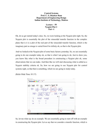
1. Control Systems
Prof. C. S. Shankar Ram
Department of Engineering Design
Indian Institute of Technology, Madras
Lecture – 59
Nyquist Plot 2
Part -1
Ok, let us get started today's class. So, we were looking at the Nyquist plot right. So, the
Nyquist plot is essentially the plot of the sinusoidal transfer function in the complex
plane that is it is a plot of the real part of the sinusoidal transfer function, which is the
imaginary part as omega is varied from 0 to infinity ok, so that is the Nyquist plot.
And we looked at the Nyquist plot of some basic factors yesterday. So, we are essentially
going to do one example today ok, so that is what I am going to do. Just to show you,
you know like what is the broad procedure in constructing a Nyquist plot ok, some
observations that we can make. And then like we will start discussing what is called as a
Nyquist stability criteria ok. So, how we are going to use Nyquist plot for control
systems right, so that that is something, which we are going to study today.
(Refer Slide Time: 01:17)
So, let me what say do an example. We are essentially going to start off with an example
in constructing the Nyquist plot. Let us say that we consider a transfer function, which is

2. of the form s plus 1 divided by s plus 10. So, the essentially the question is construct its
Nyquist plot that is the question that we are asking ourselves.
So, now how do we start doing it. You know like, so essentially first we figure out the
sinusoidal transfer function G of j omega is going to be 1 plus j omega divided by 10
plus j omega right, so that is what I am going to get. So, of course, now I what do I do, I
just multiply and divide by the conjugate of the denominator factor. So, I will get 1 plus j
omega multiplying 10 minus j omega, and this denominator will become omega square
plus 100 right, so that is what I will get ok.
So, if I now multiply, and then like simplify this, what am I going to get in the
numerator, I will get 10 plus omega square divided by omega square plus 100. And what
will be the imaginary part, it is j times 9 omega divided by omega square plus 100 right,
so that is what we will have, correct.
So, in terms of magnitude and phase, what are we going to have? So, this same thing, if I
write the magnitude and phase of the sinusoidal transfer function, the magnitude is going
to be anyway the square root of the real part square, and some plus imaginary part square
right. So, we are going to get 10 plus omega square divided by omega square plus 100
whole square plus 9 omega divided by omega square plus 100 whole square ok, so that is
the magnitude.
And what about the phase, the phase is going to be tan inverse of the imaginary
component divided by the real component. So, we will get it as 9 omega tan inverse of 9
omega divided by 10 plus omega square, am I correct right. So, these are the various
things that we will get right. So, once I once we process the sinusoidal transfer function
right.
And as we are discussing, you know like when you essentially want to plot the Nyquist
plot, what you do is that like you also create a table, and then like start plugging or
substituting different values of omega that you think are critical. And start calculating the
real part imaginary part and so on right, so that you get an idea as to what would happen
ok. So, as these what to say, these functions tend to those frequencies right.
So, let us look at omega the real part of G of j omega, and the imaginary part of G of j
omega ok. So, let us see what happens at various frequencies right. So, now if I have

3. omega to be tending to 0, what will happen, what do you think will be the real part and
the imaginary part, please note, the real part is this. What will happen to the real part as
omega tends to 0?
Student: (Refer Time: 05:02).
0.1 right, so that is what is going to happen right. So, as omega tends to 0, the real part is
going to be 0.1. What about the imaginary part, it is going to be 0. Now, as omega tends
to infinity, what do you think will happen to the real part, it will tend to 1 right. And what
will happen to the imaginary part, 0 once again right. So, if you plot the G of s plane
here, for this particular transfer function. So, this is the real axis ok, so this is the
imaginary axis, and this is the G of s plane ok.
So, let us say, we plot this sinusoidal transfer function right. So, what we are going to get
is the following right. So, let us say this is 0, so let us say this is 0.1, and let us say this is
1 all right. So, at as omega tends to 0, the transfer function values tend to I am sorry, I
think let me scroll down a little bit ok, the transfer function values, you known like value
or the transfer function tends to 0.1. And the as omega tends to infinity, the transfer
function tends to 1 ok. The real part tends to 1, imaginary part is 0.
(Refer Slide Time: 06:45)

4. So, now question is that like what happens to the locus of the what to say, this Nyquist
plot for this particular transfer function, as omega goes from 0 to infinity ok. So, please
note that, it is going to be the plot of the imaginary part, and the real part right.
So, you can see that the real part is always going to be positive, for all omega between 0
to infinity right. So, one can always see that for omega between 0 and infinity, you can
immediately see that the real part of G of j omega is always greater than 0 that is
something, which is pretty obvious right. And the imaginary part is always going to be
for omega greater than 0, it is also going to be greater than 0 right, and less than infinity.
Of course, if I put omega greater than or equal to 0, it is I have to put it as imaginary part
greater than or equal to 0 all right. So, please note what am I doing, I am taking omega
greater than 0, and less than infinity. So, so essentially the imaginary part will be
infinitesimally positive ok. So, you see that immediately the Nyquist plot is going to lie
in the?
Student: (Refer time: 07:47).
1st quadrant ok, so that is something, we can immediately see. And as I told you, you
know like by enlarge, if we go, and look at it right. So, sometimes you know like what
you can do that you can use intuition right. So, and by enlarge, when you have this first
order factors, and when you have such transfer functions, you could try out an equation
of a circle, you know like for seeing whether that will be the Nyquist plot right. So, if I
want to have a semi-circle, which whose endpoints are 0.1 and 1, what should be its
center?
Student: 0.5 (Refer Time: 08:22).
Point?
Student: (Refer Time: 08:23).
0.55 right. And what should be its radius?
Student: 0.45.
0.45, right. And it, so happens that this I leave it to you as homework ok. So, if you
check this expression, 10 plus omega square divided by omega square plus 100, which is

5. a real part, minus 0.55 whole square plus the imaginary part square, which is 9 omega
divided by omega square plus 100 the whole square that is going to be equal to 0.45
square ok. You will see that this equation is going to be satisfied right.
So, you will see that the center is somewhere here at 0.55. And we are going to have a
semi-circle ok. So, is this ok, yeah it looks like circle. Yes, any questions, ok. So, it has
the maximum value at 0.55 ok, so that is what we have right. So, this radius is going to
be 0.45 ok, so that is the what to say Nyquist plot ok. So, please do this as homework,
you know like you can double check that this is the case, this is the equation in this
scenario.
Now, if you want to find out at what omega, the phase angle of this particular sinusoidal
transfer function is maximum, how do you do that, how would you calculate the phase of
this G of j omega at any omega?
Student: (Refer time: 10:12).
Graphically let us say, you have the Nyquist plot right, what do you do?
Student: (Refer Time: 10:18).
Yeah. So, at any omega, what you do is that you draw a vector from the origin to the to
that point, and then calculate what is the angle made by that vector from the positive real
axis, in the counter clockwise direction that is taken to be positive convention right. So,
as you said if I want to figure out the maximum angle, I need I need to draw the tangent
all right.

6. (Refer Slide Time: 10:46)
So, from the origin I see, which point at which point essentially I can get a tangent to the
semi-circle right. So, essentially let us say, this is my tangent right. So, this is the omega,.
What I call as omega m is the frequency at which I get the maximum phase phi m ok. So,
phi m is the maximum phase of G of j omega right.
So, the Nyquist plot helps us with all these things. And we will see why this is important
ok. I have chosen this example with a with a motivation right. All the examples I am
choosing finally, lead to some consequence ok, we will see ok. In maybe in the next few
classes, we will see, why this is going to be important. Why did I choose this particular
example, and why am I talking about the maximum phase contribution right, or phase
angle of this particular transfer function.
So, you see that phi m is the maximum phase of G of j omega ok, omega m is a
corresponding frequency ok. Now, how can I calculate phi m, is there a way to calculate
phi m. Even using geometry, phi m is that angle right, I am sure all of us agree right. You
just using geometry, can you calculate phi m right.
Student: (Refer Time: 12:38).
Phi m is this angle right. So, see let us say of course, if I draw this, you will get the
answer right. Let us say I draw a line segment from this point to the center of the circle
semicircle right, what is the length of this line segment?

7. Student: (Refer Time: 13:00).
The radius. What can you say about the angle made by the tangent and the radius, 90.
Now you do you have the answer. What is sin phi m, this is 0.45, then so we notice that
sin phi m is going to be 0.45 divided by 0.55. Can you calculate phi m, and tell me. So,
this is 54.9.
So, essentially you can see that this is the maximum phase that is contributed by this
particular transfer function ok. And by enlarge, if this phase angle is positive, that means,
that there is a phase lead. And if the phase angle is negative, that means, there is a phase
lag ok.
So, in general so this is a just an aside ok. So, if phase is greater than 0 ok, we call it as a
positive phase right, so positive phase angle. So, it is also called as phase lead so
essentially or lead factor. So,, but if you have a negative phase angle ok, phase is greater
than less than 0 that essentially do not serve negative phase angle that is what is called as
a phase lag.
So, you see that this particular factor adds positive phase right. So, essentially it provides
a phase lead and the maximum phase lead that it can provide is around 55 degrees. We
will see why this becomes important as we go later. Please remember this ok. So, we will
we will use it later on ok.
Now, how do you find omega m?
Student: (Refer Time: 15:38).
Of course, there are you know the equation for the phase angle. And then like you plug
it in and then calculate omega m all right. You know tan phi m that is going to be 9
omega m divided by 10 plus omega m square right is it not right.

8. (Refer Slide Time: 16:06)
So, for finding omega m you know that tan phi m is going to be equal to 9 omega m
divided by 10 plus omega m square. So, if you solve this, you will get omega m to be
equal to 3.162 ok, of course, radians per second. So, you please do this as homework
once again ok. So, this is also a homework problem so that something which I wanted
right. Please do this.
And one more thing which we are going to do is an I am going to leave you with another
homework problem plot the bode diagram of this G of s which is essentially you took it
as s plus 1 divided by s plus 10. So, the same transfer function plot its bode diagram.
Please do this as homework ok, please do this and compare right. I think we have already
discussed bode diagrams in detail we have done an example in class also [, but let me get
you started. So, how do you plot the bode diagram?
Student: (Refer Time: 17:34).
Of course you need to divide into particular factors right. So, what do we do? If G of s is
going to be this, I can rewrite this as I need to rewrite in the standard form right. I can
pull 10 out from the denominator, so I am just going to get 0.1 s plus 1 divided by s by
10 plus 1 correct. Do you agree? Ok, so it has three factors.
So, this means that it has a 0.1 scalar, and then you have a s plus 1 and there is an s by 10
plus 1 ok, three factors are there. So, you plot the bode diagram for all the three

9. individual factors and then write the magnitude plot and the phase plot. So, what are the
corner frequencies of these factors? If you consider s plus 1 what is the corner frequency,
corner frequency?
Student: 1 (Refer Time: 18:43).
1? Right, and what about the corner frequency of s by 10 plus 1?
Student: (Refer Time: 18:53).
0.1 or 10?
Student: 10.
10 right, because its T s plus 1 right. So, and corner frequency is 1 by T capital T is a
coefficient of s. So, here is 1 by 10 then you take the reciprocal. So, the corner frequency
is going to be 10.
So, now can you relate 3.162 to 10 and 1 no of course, I am just playing with numbers,
but then you will see that it translates into generality for such factors right. So, so I
chosen these numbers for due to a particular motivation, which will become clear as I
told you. So, how can you relate 1 and 10 to 3.162?
Student: (Refer Time: 19:36).
Ah square root of essentially 10 and 1 right. So, when you use a logarithmic scale,
whereas 3.162 going to be? Say let us say you use a logarithmic scale right for omega.
So, you have 10 and 1 where is it going to be?
Student: (Refer Time: 20:05).
Midpoint right so exactly. Why, because if you if you want to essentially do 1 times 10
right. So, you take the log to the base 10. So, first of all you have log of square root is 1
by 2 of log correct. Do you agree? And then log of a times b is going to be log of a times
sorry log of a plus log of b. So, this is going to be of course we are doing log to the base
10.
So, what are we going to get, we are going to get the midpoint right. So, when we do this
1 in the logarithmic scale. So, you see that for this particular factor, the maximum phase

10. is going to be at the of course, what do you call as is let us say I give you two numbers,
you take the product and you take the square root of that what do you call that as?
Student: Arithmetic (Refer Time: 21:06).
Arithmetic mean?
Student: Geometric mean.
Geometric mean? Is it, or arithmetic mean or something else?
Student: Geometric mean.
Geometric mean right. So, you see that the phase that is frequency at which you get the
maximum what to say phase contribution from this is going to be at the geometric mean
of the two corner frequencies right in this particular case right, so that is what we are
getting. And this particular factor you know particular transfer function you know we
will generalize and we will use it in control design ok, so that is why I am I am doing this
in this example in so much of detail.
So, please go back you know like I cannot be what to say essentially more I cannot
emphasize this more. Please go back and draw the bode plot, because you will see that
you will need it in control design using frequency response. Kindly do that. Yeah, yes
any questions ok. So, please go back and plot the bode diagram and then compare it with
the Nyquist plot so that is what I want you to do as homework right.
So, so we see that you know like what we have done is we have looked at the frequency
response, we have looked at what to say the bode diagram or the Nyquist plot which are
two essentially methods to visualize the frequency response of a transfer functions ok.
There is a third plot which is called as a Nikolas plot which I leave it to you as
homework. So, we are not going to use that in this course, so but if you are interested
you can go back and look at that. So, once again its just a visual representation of the
sinusoidal transfer function that is about it.
Student: So, it is a geometric mean result is good for all s plus a by s plus (Refer Time:
23:00)
Ah all s plus a divided by.

11. Student: s plus b.
Ok, so a factors of this form will give you a that is what I am saying you know like I am
not going to generalize here, it depends on the value of a and b ok, we will come there.
So, please wait for a few more classes ok. So, that is why I am being careful to not to
extrapolate right now ok. Please hold on that is a good question ok. He is asking if you
take a transfer function of the form s plus a divided by s plus b right, is this result going
to hold in general, partly yes, partly no, depends on the value of a and b ok. We will see
as we go along, fine. Yeah.
Student: s plus 10 (Refer Time: 23:43).
Oh, yes, yes thank you yeah sorry about that.
(Refer Slide Time: 23:54)
Now, let me erase this yeah this should be 1 divided by s by 10 plus 1. You are right,
thank you. Yeah, sure ok, so that is what you have But then like you can also make some
general observations right. What are the values of n and m? It is essentially 1 and 1. So,
is this a minimum phase transfer function, it is right.
See, because typically see by the way I think I should highlight this point there are two
groups or two what to say ways in which people look at a minimum phase transfer
function or a minimum phase systems right. Some people associated only with the zeros
ok, because they implicitly they assume a stable system to begin with.

12. See, if you if you take any transfer function which is of the form n of s by d of s right.
How did we define a minimum phase transfer function, 1 whose zeros are in the left of
complex plane you know it was implicitly assumed that the poles are in the left of
complex plane. Because when we talk about frequency response, you recall that we are
talking about stable systems then only frequency response make sense right. So,
implicitly we are assuming all the poles to be in the left of complex plane. Another
school of thought essentially tells that you know minimum transfer function is 1 where
all its zeros and poles are in the left of complex plane ok.
So, I just wanted to highlight that difference to you these this alternative notion our
definition to you. The reason why I wrote the definition as what to say minimum transfer
function being 1, where all zeros are in the left of complex plane was that because I
implicitly assumed that all the poles are already in the left of complex plane. Is it clear
ok? So, there is a subtle difference I want wanted to a highlight.
So, this is a minimum transfer minimum phase transfer function, if you recall a minimum
phase transfer function. What does the what to say in general the slope of the high
frequency asymptote? Did you recall our do you recall our discussion? Slope of their
magnitude curve see if this is of order m, and this is of order n, what is the slope of the
high frequency asymptote?
Minus 20 times n minus m decibels per decade right. Is that satisfied here? Yes, right,
why because s plus 1 will contribute plus 20 decibels per decade; 1 divided by s by 10
plus 1 will contribute minus 20 decibels per decade. What is going to happen both are
just going to cancel out each other right that is what is going to happen that is point
number 1. And what can you say about its phase as omega tends to infinity? What is
going to happen to for a minimum phase transfer function you remember? The phase
tends to minus 90 times n minus m right.
So, this is these are the results as omega tends to infinity the magnitude tends to this 1,
the phase tends to this for a minimum phase system right. So, what is going to be the
value here 0. And Does it tend to 0? It does right because s plus 1 will give you a phase
contribution of plus 90 1 by s by 10 plus 1 will give you a phase contribution as minus
90 as omega tends to infinity. So, the sum is going to be 0. And can you observe it from

13. the Nyquist plot? You can right. Because what is the what to say transfer function, where
is the transfer function as omega tends to 0?
Student: (Refer Time: 28:09).
1
Student: (Refer Time: 28:13).
1?
Student: (Refer Time: 28:14).
Not 0.1, 1; see as omega tends to what to say infinity is this where is it at omega tending
to infinity it is at 1 right. If the transfer function is at 1, what is the angle made by that?
See how do you get the angle you draw the vector from the origin to the point right. So,
you are going to have a vector which is aligned along the positive real axis. So, what is
the angle, 0 degrees all right. So, I am just what to say we are just double checking the
results. Is it clear? Ok, so you can see that the results that we discussed hold true. Yeah.