SlideShare a Scribd company logo
1 of 22
Download to read offline
DEPTH-FIRST SEARCH OF A GRAPH 
Some Applications: 
• Finding a path between two nodes x and y (an xy-path). 
• Finding if the graph is connected. 
• Finding cut-vertices and bicomponents (maximal subgraph with-out 
a cut-vertex). 
A B 
D C 
E 
F 
(i) A connected graph 
on nodes {A, B, ×××, F}. 
A B 
D C 
E 
F 
(ii) A disconnected graph 
on nodes {A, B, ×××, F}. 
Connected graph: 
• There is a path between each pair of nodes x and y (y ¹ x). 
Question: 
•? What are the simple (acyclic) DE-paths for the graph on left? 
•? If there is path from some node z to every other node, then is it 
true that there is a path between every pair of nodes x and y ¹ x? 
•? Why is this result important? 
Cut-vertex x: 
• Removal of x and its adjacent edges destroys all paths (³ 1) 
between some pair of nodes y and z; we say x separates y and z. 
Question: 
•? What are the cut-vertices in the above graphs. 
•? What is the minimum number edges that need to be added to the 
first graph so that it has no cut-vertex.
2.2 
DEPTH-FIRST TREE 
Spanning Tree (of a connected graph): 
• Tree spanning all vertices (= n of them) of the graph. 
• Each spanning tree has n nodes and n - 1 links. 
Back-Edges and Cross-Edges (for a rooted spanning tree T): 
• Anon-tree edge is one of the following: 
- back-edge (x, y): joins x to ancestor y ¹ parent(x). 
- cross-edge (x, y): other non-tree edges. 
A B 
D C 
E 
F 
H G 
(i) Solid lines show 
a spannig tree 
A root 
B H 
C E 
F 
G 
D 
(ii) Dashed lines show back-edges; no cross-edges. 
Tree edges directed from parent to child. 
Depth-First Tree: 
• Arooted spanning tree with no cross-edges (as in (ii) above). 
Question: 
•? Show the back-edges and cross-edges if B is the root. Is this a 
depth-first tree (why)? Do the same for root = E and root = F. 
•? Show all spanning trees of the graph below (keep the nodes in 
the same relative positions). 
A B 
D C
2.3 
VISITING EDGES IN A 
DEPTH-FIRST TRAVERSAL 
A B 
D C 
E 
F 
H G 
adjList(A) = áB, C, F, Hñ 
adjList(B) = áA, C, E, G, Dñ 
adjList(C) = áA, Bñ, adjList(D) = áB, Gñ 
adjList(E) = áB, Fñ, adjList(F) = áA, Eñ 
adjList(G) = áB, Dñ, adjList(H) = áAñ 
A 1, root 
2 B H 8 
3 C 4 E 
5 F 
G 6 
D 7 
(ii) The dfTree, dfLabels, 
and back-edges. 
Order of Processing Links and Backtracking: StartNode = A. 
(A, B) tree-edge (G, B) 2nd visit 
(B, A) 2nd visit (G, D) tree-edge 
(B, C) tree-edge (D, B) back-edge 
(C, A) back-edge (D, G) 2nd visit 
(C, B) 2nd visit backtrack D®G 
backtrack C®B backtrack G®B 
(B, E) tree-edge (B, D) 2nd visit 
(E, B) 2nd visit backtrack B®A 
(E, F) tree-edge (A, C) 2nd visit 
(F, A) back-edge (A, F) 2nd visit 
(F, E) 2nd visit (A, H) tree-edge 
backtrack F®E (H, A) 2nd visit 
bacltrack E®B backtrack H®A 
(B, G) tree-edge backtrack A® 
Two Basic Operations: Move forward and backtrack. 
Question: 
•? Show the order of processing the links and backtracking if we 
reorder adjList(A) = áF, B, C, Hñ for the above graph.
2.4 
USE OF STACK AND DEPTH-FIRST LABEL 
FOR DEPTH-FIRST TRAVERSAL 
A B 
D C 
E 
F 
H G 
adjList(A) = áB, C, F, Hñ 
adjList(B) = áA, C, E, G, Dñ 
adjList(C) = áA, Bñ, adjList(D) = áB, Gñ 
adjList(E) = áB, Fñ, adjList(F) = áA, Eñ 
adjList(G) = áB, Dñ, adjList(H) = áAñ 
A 1, root 
2 B H 8 
3 C 4 E 
5 F 
G 6 
D 7 
(ii) The dfTree, dfLabels, 
and back-edges. 
Stack Node LastDf-or 
Link Label Processing 
áAñ A 0 ®1 dfLabel(A) = 1, nextNode = B = adjList(A, 0), 
nextToVisit(A) = 1¬0 
(A, B) tree-edge, parent(B) = A, add B to stack 
áA, Bñ B 1 ®2 dfLabel(B) = 2, nextNode = A = adjList(B, 0), 
nextToVisit(B) = 1¬0 
(B, A) second-visit, nextNode = C = adjList(B, 1), 
nextToVisit(B) = 2¬1 
(B, C) tree-edge, parent(C) = B, add C to stack 
áA, B, Cñ C 2 ®3 dfLabel(C) = 3, nextNode = A = adjList(C, 0), 
nextToVisit(C) = 1¬0 
(C, A) back-edge, nextNode = B = adjList(C, 1), 
nextToVisit(C) = 2¬1, 
(C, B) second-visit, backtrack 
áA, Bñ B nextNode = E = adjList(B, 2), 
nextToVisit(B) = 3¬2 
(B, E) tree-edge, parent(E) = B, add E to stack 
áA, B, Eñ E 3 ®4 dfLabel(E) = 4, nextNode = B = adjList(E, 0), 
nextToVisit(E) = 1¬0 
(E, B) second-visit, nextNnode = F = adjList(E, 1), 
nextToVisit(E) = 2¬1 
(E, F) tree-edge, parent(F) = E = adjList(E, 1), 
nextToVisit(E) = 3¬2 
××× ××× ××× ×××
2.5 
DATA-STRUCTURES IN 
DEPTH-FIRST TRAVERSAL ALGORITHM 
Array Data-Structures (each array-size = numNodes): 
dfLabels[i]: the depth-first label (³ 1) assigned to node i; 
each dfLabels[i] = 0, initially. 
nextToVisits[i]: nextToVisits[i] gives the position of the item 
in adjList of node i that is to be visited next 
from node i; each nextToVisit[i] = 0, initially; 
parents[i]: the parent of node i in depth-first tree; par-ents[ 
startNode] = startNode, initially. 
Additional Data-Structures: 
• lastDfLabel = 0, initially; 
it is incremented by one before assigning it to a node. 
• stack[0..numNodes-1]; 
it is initialized with the startNode and it contains the path in the 
depth-first tree from the root to the current node = top(stack). 
Notes: 
• You can add parent, dfLabel, and nextToVisit information in the 
structure GraphNode as shown below. 
typedef struct { 
int degree, *adjList, //arraySize = degree 
nextToVisit, //0<=nextToVisit<degree 
parent, dfLabel; 
} GraphNode; 
In that case, the next link to visit from node i is link (i, j), where 
j = nodes[i].adjList[nodes[i].nextToVisit]; otherwise, j = 
nodes[i].adjList[nextToVisit[i]].
2.6 
PSEUDOCODE FOR 
DEPTH-FIRST TRAVERSAL ALGORITHM 
First Version: 
1. Try to go down the tree (which is being created) from the current 
node x by choosing a link (x, y) in the graph from x to a node y 
not yet visited and adding the link (x, y) to the tree. 
2. If there is no such node y, then backtrack to the parent of the 
current node, and stop when you backtrack from the startNode 
(= root of the tree). 
AMore Detailed Version (with parents[] and nextToVisit[]): 
1. Initialize the arrays parents[] and nextToVisit[] as indicated in 
the previous page and let currentNode = startNode. 
2. Search adjList[currentNode] from the position nextToVisit[cur-rentNode] 
onwards for a nextNode which is not yet visited, 
3. [Move forward.] If (nextNode is found), then let parents[nextN-ode] 
= currentNode, update nextToVisit[currentNode], and cur-rentNode 
= nextNode. 
4. [Backtrack.] If (no nextNode is found) then do the following: 
(i) If (currentNode = startNode) then stop. 
(ii) Otherwise backtrack, i.e., let currentNode = parents[cur-rentNode] 
and goto step (2).
2.7 
DEPTH-FIRST TRAVERSAL ALGORITHM 
Algorithm DepthFirstTraverse: 
Input: A graph in adj-list form and a start-node. 
Output: A depth-first spanning tree for the connected 
component containing start-node. 
1. Initialize lastDfLabel, the stack, and also the arrays dfLabels, 
parents, and nextToVisits as indicated in the previous page. 
2. While (stack ¹ empty) do the following: 
(a) Let currentNode = top(stack) and if (dfLabels[currentNode] 
= 0) then update lastDfLabel and let dfLabels[currentNode] 
= lastDfLabel. 
(b) If (nextToVisit[currentNode] = degree[currentNode]) then 
backtrack by removing top of stack. 
(c) Otherwise, let nextNode = the node in position nextTo- 
Visit[currentNode] in adjList(currentNode), and update 
nextToVisit[currentNode]. 
Classify the link (currentNode, nextNode) as follows 
searching for a tree-edge (if any) from currentNode: 
(i) if (dfLabels[nextNode] = 0) then it is a tree-edge; let 
parent[nextNode] = currentNode, add nextNode to 
stack. 
(ii) if (dfLabels[nextNode] < dfLabels[currentNode]) then 
if (nextNode ¹ parents[currentNode]) then it is a back-edge 
and otherwise it is a second visit of tree-edge. 
(iii) Otherwise, it is a second visit to a back-edge. 
Note: We merged old (c)-(d), eliminated all goto’s and putting 
(c)-(d) in a loop, and split d(ii) into d(ii)-(iii). Also, added 
an if-part in (a).
2.8 
EXERCISE 
1. How many times a link (x, y) is visited and when? 
2. What is the total number of back-edges? 
3. How many tree-edges and back-edges are there at a node x? 
4. How many times does a node x enter the stack and when? 
5. How many times do we backtrack to a node x? How many 
times do we backtrack from a node x and when? 
6. Shown below is a graph and a depth-first tree for startNode = 
A. 
A B 
D C 
E 
F 
H G 
(i) A graph. 
A root 
B H 
C E 
F 
G 
D 
(ii) A depth-first tree. 
(a) Show all possible orderings of the adjacency list of A 
which will give this tree when we apply the depth-first tra-versal 
algorithm. Do the same for node B, keeping startN-ode 
= A. 
(b) Give the total number of ways of ordering the various 
adjacency lists which will give the above depth-first tree. 
(c) Arrange all adjacency-lists in such a way that at each node 
x, the tree-edges from x to its children are visited first, 
then the back-edges from x (if any, to its ancestors), next 
the second-visit of tree-edge connecting x to its parent (if 
any), and finally the second-visit of back-edges to x (if 
any, from its descendants).
2.9 
7. How do you distinguish a second-visit to a tree edge vs. a sec-ond- 
visit to a backedge? 
8. For each edge processed in the table on page 3, show the asso-ciated 
step of the algorithm on page 7 that is used for it. 
9. Show the modifications to the delth-first traversal algorithm to 
compute maxDfLabel(x) = max {dfLabel(y): y = x or a 
descendant of x} for each node x. Use the depth-first tree 
above to explain how this works. How can you compute the 
size of the subtree at x using maxDfLabel(x)? 
10. Is it true that the nodes in the subtree at x of a depth-first tree 
consists of all nodes that can be reached from x without using 
any of the other nodes on the path from root to x?
2.10 
A RECURSIVE VERSION 
OF DF-TRAVERSAL 
Notes: 
• Backtracking corresponds to return from the recursion. 
• The lastDfLabel and the dfLabels-array can be static in DF-TRAVERSAL; 
the nextToVisit-array is not used. 
• The recursive-call at x creates the subtree of df-tree at x as we 
build the df-tree via child-pointers, etc. 
Algorithm DF-TRAVERSAL(currNode): //first call: currNode = s 
Input: A graph in adj-List form and a start-node s. 
Output: The df-tree, with root = s. 
1. [Create df-tree node.] Create currTreeNode in df-tree for currN-ode. 
If (lastDfLabel = 0), then initialize dfLabel(x) = 0 for each 
x and let parent(currTreeNode) = currTreeNode. Now, let dfLa-bel( 
currNode) = lastDfLabel = lastDfLabel + 1. 
2. For (each node x in adjList(currNode)) do the following: 
If (dfLabel(x) = 0) then add the root-node (which corre-sponds 
to x) of the subtree returned by DF-SEARCH(x) as 
the next child of currTreeNode. 
3. Return(currTreeNode). 
Complexity: O(|V| + |E|) = O(|E|) for a connected G. 
• An edge (x, y) is examined at most once in each direction. 
• Aconstant amount of work per node x (assigning dfLabel(x), 
adding x to the df-tree, and backtracking from x).
2.11 
ILLUSTRATION OF THE RECURSIVE 
DF-TRAVERSAL 
L A 
K A/1 
B J 
B/2 J/3 
K/4 
L/5 
DF-TRAVERSAL(A) 
parent(A) = A 
dfLabel(A) = 1 
= lastDfLabel 
parent(B) = A 
DF-TRAVERSAL(B) 
dfLabel(B) = 2 
= lastDfLabel 
parent(J) = A 
DF-TRAVERSAL(J) 
dfLabel(J) = 3 
= lastDfLabel 
parent(K) = J 
DF-TRAVERSAL(K) 
dfLabel(K) = 4 
= lastDfLabel 
parent(L) = A 
DF-TRAVERSAL(L) 
dfLabel(L) = 5 
= lastDfLabel 
• #(calls to DF-TRAVERSAL) = #(nodes in df-tree) = #(nodes in 
graph), if G is connected. 
• #(direct calls from DF-TRAVERSAL(x)) = #(children x).
2.12 
A SAMPLE OUTPUT OF 
DF-TRAVERSAL PROGRAM 
L 4 3 K 
A 0 
B 1 2 J 
Input Graph: 
numNodes = 5 
0 (4): 1 2 3 4 
1 (1): 0 
2 (2): 0 3 
3 (2): 0 2 
4 (1): 0 
------------------------------ 
startNode = 0, dflabel(0) = 1 
processing (0,1): tree-edge, dfLabel(1) = 2 
processing (1,0): tree-edge 2nd-visit 
backtracking 1 -> 0 
processing (0,2): tree-edge, dfLabel(2) = 3 
processing (2,0): tree-edge 2nd-visit 
processing (2,3): tree-edge, dfLabel(3) = 4 
processing (3,0): back-edge 
processing (3,2): tree-edge 2nd-visit 
backtracking 3 -> 2 
backtracking 2 -> 0 
processing (0,3): back-edge 2nd-visit 
processing (0,4): tree-edge, dfLabel(4) = 5 
processing (4,0): tree-edge 2nd-visit 
backtracking 4 -> 0 
------------------------------ 
PROGRAMMING EXERCISE 
1. Create a function depthFirstTraverse(int startNode). It should 
produce output as indicated above. Use an auxiliary function 
readGraph (input file should be in the same form as for a digraph 
using adjacency-lists), which should output the graph read. keep 
the adjacency lists sorted in increasing order. Show the output 
for the 8 node graph on page 2.2 with startNode B (= 1).
2.13 
NODE-STRUCTURE FOR 
AN ORDERED-TREE 
• The parent-links alone do not allow us to traverse the df-tree 
from the root (= startNode of depth-first traversal). 
• Since the number of children of a node is known ahead of time, 
the children are kept in a linked-list. 
• The lastChild pointer helps addition of a child and firstChild 
pointer accessing the children. 
typedef struct TreeNode { 
int node, numChildren; 
struct TreeNode *parent, 
*leftBroth, *rightBroth, 
*firstChild, *lastChild; 
} TreeNode; 
parent(x) 
leftBroth(x) x 
rightBroth(x) 
firstChild(x) lastChild(x) 
Example. Null-pointers not shown; firstChild(J) = lastChild(J). 
The nodes are numbered 0, 1, ××× in alpabetical order. 
A/0; 3 
B/1; 0 J/2; 1 L/4; 0 
K/3; 0 
firstChild 
lastChild 
parent 
rightBroth 
leftBroth
2.14 
ALL ACYCLIC PATHS IN A GRAPH 
FROM A START-NODE 
Example. Shown below is a graph and the tree of all acyclic paths 
from a. 
a b 
d c 
e 
(i) A graph G. 
a 
b 
c 
d 
e 
d 
c e 
d 
b 
c 
c 
b 
e 
e 
d 
b 
c 
c 
b 
(ii) The tree of acyclic paths from a in G. 
Some Properties of this Tree (startNode = s): 
• Anode x appears in the tree as many times as the number of 
acyclic paths to x from s. 
• We can find all cycles (without repetition of nodes) at a node s 
from these paths: 
- Combine an sx-path with the edge (s, x), if exists. 
- Each cycle is obtained twice in this process, once in each 
direction. 
• We can find if there is a Hamiltonian cycle (cycle containing all 
nodes exactly once). 
Note: 
• To deremine all acyclic paths from startNode, use the depth-first 
traversal with the change: reset nextToVisit[i] = 0 = dfLabel[i] in 
backtrack from node i.
2.15 
OBJECT-REGION IN A BINARY-IMAGE 
Binary-image: 
• Anm´narray, where a pixel pij = 1 (shown below as a shaded 
square) represents a part of an object in the image; a pixel pij = 0 
represents a part of the background. 
A 6´6 binary image. 
Adjacent Pixels: 
• Two 1-pixels are adjacent if they share an edge. 
• Two 0-pixels are adjacent if they share a corner or an edge. 
pi-1, j 
pi, j-1 pi, j pi, j+1 
pi+1, j 
At most 4 neighbors of 
an 1-pixel pij . 
pi-1, j 
pi, j-1 pi, j pi, j+1 
pi+1, j 
At most 8 neighbors of 
a 0-pixel pij . 
Image-object: A maximal set of connected 1-pixels pij . 
Example. The above image has 2 objects of sizes 7 and 4 and two 
background regions of sizes 1 and 24. 
Question: Give a 5´5 image with maximum number of objects.
2.16 
OBJECT DETERMINATION 
BY DF-TRAVERSAL 
Order of Visit of Neighbors of 1-pixel pij (if present): 
(1) pi, j+1 (E-neighbor) (3) pi, j-1 (W-neighbor) 
(2) pi-1, j (N-neighbor) (4) pi+1, j (S-neighbor) 
Additional Backtracking Rule: 
• If we reach a 0-pixel, we immediately backtrack. 
Example. Shown below is the depth-first labeling of the pixels vis-ited 
starting at the position labeled 1. 
All neighboring 0-pixels of the region R containing the 
start-pixel are also visited. The total number of visits to 
those 0-pixels is at most 2(|R| + 1) - why? 
7 
5 6 
9 3 4 
1 2 
14 
8 
10 
12 11 
13 15 
18 16 17 
start-pixel 
1 
2 
E 
3 
N 
4 
E 
5 
N 
6 
E 
7 
N 
8 
W 
9 
W 
8 
N 
W 
10 
W 
11 
S 
E 
W 
12 
S 
13 
14 
S 
15 
E 
W 
13 
16 
S 
E 
17 
W 
18 
The dashed lines indicate 
neighbor that are visited 
but are not in the current 
region. These nodes appear 
as many times as they are 
visited, each time causing 
an immediate backtracking; 
both nodes 8 and 13 appear 
here twice.
2.17 
INTERNAL AND EXTERNAL BOUNDARIES 
OF AN OBJECT 
Non-Boundary (internal) Pixel p of An Object: 
• Completely surrounded by 8-neighbor object pixels. 
p 
Two Types of Background Pixels: 
• 0-regions are based on 8-neighbors. 
• External regions: 0-regions which contain at least one pixel in 
the first or last row or first or last column. 
• Holes: other 0-regions completely surrrounded by object pixels; 
does not contain pixels from first (last) row or column. 
´ ´ ´ ´ 
´ ´ 
´ ´ 
´ ´ ´ ´ 
Two holes of 
sizes 2 and 3. 
Two external 
regions of 
sizes 3 and 15. 
Internal pixel of the object 
Only external boundary pixels 
Only internal boundary pixels 
´ Both internal and external 
boundary pixels 
Two Types of Boundary (non-internal) Pixels: 
• Internal boundary: Objects pixels adjacent to holes (based on 
8-neighbors). 
• External boundary: Object pixels adjacent (based on 8-neigh-bors) 
to external regions or in the first (last) row or column. 
Question: Show the boundary and internal pixels if the pixel p5,4 
above were a 0-pixel (merging two holes into one),
2.18 
VISITING A MAZE OR 
EXTERNAL BOUNDARY OF AN OBJECT 
Strategy: 
• Keep to the right, starting at a southmost pixel of maze or object. 
• Assume that we arrived at the start-position with a north-move 
(thus, attempt to go east first at start-position). 
Start-point 
Part of the move sequence visiting a maze. 
The trail of "return visits" parts are shown in bold. 
The move sequence visiting the external boundary of an object. 
Question: Show the move sequence if we start at pixel p3,3.
2.19 
OBJECT SIMPLIFICATION 
BY FILLING UP HOLES IN THE OBJECT 
An image with three objects. 
The largest object contains 
two holes and one of the objects 
is placed in one of those holes. 
The non-boundary pixels of this 
object are shown in light shade. 
• 
• 
• 
External Regions: 
• The 0-regions which contain at least one 0-pixel from any of 
top/bottom rows and leftmost/rightmost columns. 
Holes: These are 0-regions other than the external regions. 
After filling-in the two holes 
in the largest object. 
This swallows the third object 
in one of those holes. 
• 
• 
Questions: 
1? Show df-labels of pixels in the 0-region in the top image starting 
at p1,1 (top-left pixel); do not label 1-pixels that may be visited. 
2? Give a psuedocode to detect the pixels in the holes of an object. 
What is the computational complexity? 
3? Mark successively as 1, 2, ××× for the first visit to the 1-pixels 
starting at the southmost pixel p11,10 ( p1,1 = the top-left pixel) of 
the largest object in the top figure and using the rule "keep to the 
right". The next pixel visited would be p10,10. (Note: there is no 
backtracking here, and some pixel may be visited more than 
once. As usual, assume we arrived at p11,10 by going north.)
2.20 
TREE OF SHORTEST-PATHS IN DIGRAPHS 
C 
3 1 
D 
2 1 
5 
A 2 B 
1 E 
1 
5 
A digraph 
®G 
with 
each c(x, y) ³ 0. 
Start-node s = A. 
• 
• 
A 
2 B 
5 C 
10 D 
E 3 
C 8 
D 13 
D 1 E 1 
C 6 
7 B D 11 
• Bold links show the 
tree of shortest-paths 
to various nodes. 
The tree of acyclic paths from A; shown next to 
each node is the length of the path from root = A. 
Some Important Observations: 
• Any subpath of a shortest path is a shortest path. 
• The shortest paths from a startNode to other nodes can be chosen 
so that they form a tree. 
Question: 
•? What are some minimum changes to the link-costs that will 
make áA, B, E, Cñ the shortest AC-path? 
•? Show the new tree of acyclic paths ad the shortest paths from 
startNode = A after adding the link (D, B) with cost 1. 
•? Also show the tree of acyclic paths and the shortest paths from 
the startNode = D.
2.21 
ILLUSTRATION OF 
DIJKSTRA’S SHORTEST-PATH ALGORITHM 
C 
3 1 
D 
1 
1 
A 2 B 
2 
5 
1 E 
1 
5 
d(x) = length of best path known to x 
from the startNode = A. 
A node is closed if shortest 
path to it known. 
A node is OPEN if a path to it known, 
but no shortest path is known. 
• 
• 
• 
"?,?" indicates unknown values, "×××" indicates no changes, and 
"-" indicates path-length not computed (would not have changed any way). 
Open Node Links d(x) and parent(x) 
Nodes Closed processed A B C D E 
{A} Æ 0, A ?, ? ?, ? ?, ? ?, ? 
{B} A (A, B) 2, A 
{B, D} (A, D) 1, A 
{B, D, E} (A,E) 1, A 
{B, E} D (D, A) - 
(D, B) ××× 
{B, C} E (E, C) 6, E 
{C} B (B, C) 5, B 
(B, E) - 
Æ C (C, B) - 
(C, D) - 
Question: 
•? List all paths from A that are looked at (length computed) above. 
•? When do we look at a link (x, y)? How many times do we look 
at a link (x, y)? 
•? What might happen if some c(x, y) < 0?
2.22 
DIJKSTRA’S ALGORITHM 
Terminology (OPENÇCLOSED = Æ): 
CLOSED = {x: p m(s, x) is known}. 
OPEN = {x: some p (s, x) is known but x ÏCLOSED}. 
Algorithm DIJKSTRA (shortest paths from s): 
Input: AdjList(x) for each node x in 
®G 
, each c(x, y) ³ 0, a 
start-node s, and possibly a goal-node g. 
Output: A shortest sg-path (or sx-path for each x reachable 
from s). 
1. [Initialize.] d(s) = 0, mark s OPEN, parent(s) = s (or NULL), 
and all other nodes are unmarked. 
2. [Choose a new closing-node.] If (no OPEN nodes), then there is 
no sg-path and stop. Otherwise, choose an OPEN node x with 
the smallest d(×), with preference for x = g. If x = g or all but 
one node are closed, then stop. 
3. [Close x and Expand p m(s, x).] Mark x CLOSED and for (each 
y ÎadjList(x) and y not marked CLOSED) do: 
if (y not marked OPEN or d(x)+c(x, y) < d(y)) then let par-ent( 
y) = x, d(y) = d(x) + c(x, y), and mark y OPEN. 
4. Go to step (2). 
Complexity: O(N2). 
• A node x is marked CLOSED at most once and hence a link 
(x, y) is processed at most once. 
• Each iteration of steps (2) and (3) takes O(N) time.

More Related Content

What's hot

3.1 higher derivatives
3.1 higher derivatives3.1 higher derivatives
3.1 higher derivatives
math265
 
บทที่ 4 ฟังก์ชัน
บทที่ 4 ฟังก์ชันบทที่ 4 ฟังก์ชัน
บทที่ 4 ฟังก์ชัน
Thipayarat Mocha
 
52 notation and algebra of functions
52 notation and algebra of functions52 notation and algebra of functions
52 notation and algebra of functions
math126
 
19 min max-saddle-points
19 min max-saddle-points19 min max-saddle-points
19 min max-saddle-points
math267
 
0101: Graphing Quadratic Functions
0101: Graphing Quadratic Functions0101: Graphing Quadratic Functions
0101: Graphing Quadratic Functions
kijo13
 

What's hot (18)

3.1 higher derivatives
3.1 higher derivatives3.1 higher derivatives
3.1 higher derivatives
 
Cubic BF-Algebra
Cubic BF-AlgebraCubic BF-Algebra
Cubic BF-Algebra
 
C3 Transformations
C3 TransformationsC3 Transformations
C3 Transformations
 
บทที่ 4 ฟังก์ชัน
บทที่ 4 ฟังก์ชันบทที่ 4 ฟังก์ชัน
บทที่ 4 ฟังก์ชัน
 
Functions
FunctionsFunctions
Functions
 
The Quadratic Function Derived From Zeros of the Equation (SNSD Theme)
The Quadratic Function Derived From Zeros of the Equation (SNSD Theme)The Quadratic Function Derived From Zeros of the Equation (SNSD Theme)
The Quadratic Function Derived From Zeros of the Equation (SNSD Theme)
 
F4 c1 functions__new__1_
F4 c1 functions__new__1_F4 c1 functions__new__1_
F4 c1 functions__new__1_
 
Functions & graphs
Functions & graphsFunctions & graphs
Functions & graphs
 
Red black 2
Red black 2Red black 2
Red black 2
 
52 notation and algebra of functions
52 notation and algebra of functions52 notation and algebra of functions
52 notation and algebra of functions
 
Lec 03 - Combinational Logic Design
Lec 03 - Combinational Logic DesignLec 03 - Combinational Logic Design
Lec 03 - Combinational Logic Design
 
1. functions
1. functions1. functions
1. functions
 
Graph functions
Graph functionsGraph functions
Graph functions
 
Graph a function
Graph a functionGraph a function
Graph a function
 
19 min max-saddle-points
19 min max-saddle-points19 min max-saddle-points
19 min max-saddle-points
 
Learning to score
Learning to scoreLearning to score
Learning to score
 
0101: Graphing Quadratic Functions
0101: Graphing Quadratic Functions0101: Graphing Quadratic Functions
0101: Graphing Quadratic Functions
 
Form 4 add maths note
Form 4 add maths noteForm 4 add maths note
Form 4 add maths note
 

Viewers also liked

Back tracking and branch and bound class 20
Back tracking and branch and bound class 20Back tracking and branch and bound class 20
Back tracking and branch and bound class 20
Kumar
 

Viewers also liked (20)

Algorithm in discovering and correcting words errors in a dictionary or any w...
Algorithm in discovering and correcting words errors in a dictionary or any w...Algorithm in discovering and correcting words errors in a dictionary or any w...
Algorithm in discovering and correcting words errors in a dictionary or any w...
 
Fun with Mazes
Fun with MazesFun with Mazes
Fun with Mazes
 
Backtracking Algorithmic Complexity Attacks Against a NIDS
Backtracking Algorithmic Complexity Attacks Against a NIDSBacktracking Algorithmic Complexity Attacks Against a NIDS
Backtracking Algorithmic Complexity Attacks Against a NIDS
 
Branch and bound
Branch and boundBranch and bound
Branch and bound
 
Backtracking
Backtracking  Backtracking
Backtracking
 
July 2014: About Backtrack
July 2014: About BacktrackJuly 2014: About Backtrack
July 2014: About Backtrack
 
Backtrack manual Part1
Backtrack manual Part1Backtrack manual Part1
Backtrack manual Part1
 
Backtrack
BacktrackBacktrack
Backtrack
 
Backtraking optimziation algorithm
Backtraking optimziation algorithmBacktraking optimziation algorithm
Backtraking optimziation algorithm
 
Backtracking
BacktrackingBacktracking
Backtracking
 
Backtrack os 5
Backtrack os 5Backtrack os 5
Backtrack os 5
 
Backtracking
BacktrackingBacktracking
Backtracking
 
Breadth-First Search, Depth-First Search and Backtracking Depth-First Search ...
Breadth-First Search, Depth-First Search and Backtracking Depth-First Search ...Breadth-First Search, Depth-First Search and Backtracking Depth-First Search ...
Breadth-First Search, Depth-First Search and Backtracking Depth-First Search ...
 
Backtracking
BacktrackingBacktracking
Backtracking
 
Computer Programming - Lecture 2
Computer Programming - Lecture 2Computer Programming - Lecture 2
Computer Programming - Lecture 2
 
Back tracking and branch and bound class 20
Back tracking and branch and bound class 20Back tracking and branch and bound class 20
Back tracking and branch and bound class 20
 
backtracking algorithms of ada
backtracking algorithms of adabacktracking algorithms of ada
backtracking algorithms of ada
 
Algorithm Class is a Training Institute on C, C++, CPP, DS, JAVA, data struct...
Algorithm Class is a Training Institute on C, C++, CPP, DS, JAVA, data struct...Algorithm Class is a Training Institute on C, C++, CPP, DS, JAVA, data struct...
Algorithm Class is a Training Institute on C, C++, CPP, DS, JAVA, data struct...
 
Intrusion detection and prevention system
Intrusion detection and prevention systemIntrusion detection and prevention system
Intrusion detection and prevention system
 
Backtracking
BacktrackingBacktracking
Backtracking
 

Similar to 2 depth first

FINAL PROJECT, MATH 251, FALL 2015[The project is Due Mond.docx
FINAL PROJECT, MATH 251, FALL 2015[The project is Due Mond.docxFINAL PROJECT, MATH 251, FALL 2015[The project is Due Mond.docx
FINAL PROJECT, MATH 251, FALL 2015[The project is Due Mond.docx
voversbyobersby
 
Introduction to Treewidth
Introduction to TreewidthIntroduction to Treewidth
Introduction to Treewidth
ASPAK2014
 
09 logic programming
09 logic programming09 logic programming
09 logic programming
saru40
 
graphin-c1.pnggraphin-c1.txt1 22 3 83 44 5.docx
graphin-c1.pnggraphin-c1.txt1 22 3 83 44 5.docxgraphin-c1.pnggraphin-c1.txt1 22 3 83 44 5.docx
graphin-c1.pnggraphin-c1.txt1 22 3 83 44 5.docx
whittemorelucilla
 

Similar to 2 depth first (20)

DS MCQS.pptx
DS MCQS.pptxDS MCQS.pptx
DS MCQS.pptx
 
Review session2
Review session2Review session2
Review session2
 
Cs6660 compiler design november december 2016 Answer key
Cs6660 compiler design november december 2016 Answer keyCs6660 compiler design november december 2016 Answer key
Cs6660 compiler design november december 2016 Answer key
 
Chap 5 Tree.ppt
Chap 5 Tree.pptChap 5 Tree.ppt
Chap 5 Tree.ppt
 
DSA (Data Structure and Algorithm) Questions
DSA (Data Structure and Algorithm) QuestionsDSA (Data Structure and Algorithm) Questions
DSA (Data Structure and Algorithm) Questions
 
Purely Functional Data Structures in Scala
Purely Functional Data Structures in ScalaPurely Functional Data Structures in Scala
Purely Functional Data Structures in Scala
 
FINAL PROJECT, MATH 251, FALL 2015[The project is Due Mond.docx
FINAL PROJECT, MATH 251, FALL 2015[The project is Due Mond.docxFINAL PROJECT, MATH 251, FALL 2015[The project is Due Mond.docx
FINAL PROJECT, MATH 251, FALL 2015[The project is Due Mond.docx
 
Lesson 25: Evaluating Definite Integrals (Section 10 version)
Lesson 25: Evaluating Definite Integrals (Section 10 version)Lesson 25: Evaluating Definite Integrals (Section 10 version)
Lesson 25: Evaluating Definite Integrals (Section 10 version)
 
Lesson 5: Functions and surfaces
Lesson 5: Functions and surfacesLesson 5: Functions and surfaces
Lesson 5: Functions and surfaces
 
Introduction to Treewidth
Introduction to TreewidthIntroduction to Treewidth
Introduction to Treewidth
 
ISI MSQE Entrance Question Paper (2008)
ISI MSQE Entrance Question Paper (2008)ISI MSQE Entrance Question Paper (2008)
ISI MSQE Entrance Question Paper (2008)
 
Lesson 25: Evaluating Definite Integrals (Section 4 version)
Lesson 25: Evaluating Definite Integrals (Section 4 version)Lesson 25: Evaluating Definite Integrals (Section 4 version)
Lesson 25: Evaluating Definite Integrals (Section 4 version)
 
Roots T
Roots TRoots T
Roots T
 
2 homework
2 homework2 homework
2 homework
 
Trees in Data Structure
Trees in Data StructureTrees in Data Structure
Trees in Data Structure
 
7 functions
7   functions7   functions
7 functions
 
Trees, Binary Search Tree, AVL Tree in Data Structures
Trees, Binary Search Tree, AVL Tree in Data Structures Trees, Binary Search Tree, AVL Tree in Data Structures
Trees, Binary Search Tree, AVL Tree in Data Structures
 
09 logic programming
09 logic programming09 logic programming
09 logic programming
 
graphin-c1.pnggraphin-c1.txt1 22 3 83 44 5.docx
graphin-c1.pnggraphin-c1.txt1 22 3 83 44 5.docxgraphin-c1.pnggraphin-c1.txt1 22 3 83 44 5.docx
graphin-c1.pnggraphin-c1.txt1 22 3 83 44 5.docx
 
Chapter 1 MATLAB Fundamentals easy .pptx
Chapter 1 MATLAB Fundamentals easy .pptxChapter 1 MATLAB Fundamentals easy .pptx
Chapter 1 MATLAB Fundamentals easy .pptx
 

Recently uploaded

introduction-to-automotive Andoid os-csimmonds-ndctechtown-2021.pdf
introduction-to-automotive Andoid os-csimmonds-ndctechtown-2021.pdfintroduction-to-automotive Andoid os-csimmonds-ndctechtown-2021.pdf
introduction-to-automotive Andoid os-csimmonds-ndctechtown-2021.pdf
VishalKumarJha10
 
CHEAP Call Girls in Pushp Vihar (-DELHI )🔝 9953056974🔝(=)/CALL GIRLS SERVICE
CHEAP Call Girls in Pushp Vihar (-DELHI )🔝 9953056974🔝(=)/CALL GIRLS SERVICECHEAP Call Girls in Pushp Vihar (-DELHI )🔝 9953056974🔝(=)/CALL GIRLS SERVICE
CHEAP Call Girls in Pushp Vihar (-DELHI )🔝 9953056974🔝(=)/CALL GIRLS SERVICE
9953056974 Low Rate Call Girls In Saket, Delhi NCR
 
TECUNIQUE: Success Stories: IT Service provider
TECUNIQUE: Success Stories: IT Service providerTECUNIQUE: Success Stories: IT Service provider
TECUNIQUE: Success Stories: IT Service provider
mohitmore19
 

Recently uploaded (20)

OpenChain - The Ramifications of ISO/IEC 5230 and ISO/IEC 18974 for Legal Pro...
OpenChain - The Ramifications of ISO/IEC 5230 and ISO/IEC 18974 for Legal Pro...OpenChain - The Ramifications of ISO/IEC 5230 and ISO/IEC 18974 for Legal Pro...
OpenChain - The Ramifications of ISO/IEC 5230 and ISO/IEC 18974 for Legal Pro...
 
%in ivory park+277-882-255-28 abortion pills for sale in ivory park
%in ivory park+277-882-255-28 abortion pills for sale in ivory park %in ivory park+277-882-255-28 abortion pills for sale in ivory park
%in ivory park+277-882-255-28 abortion pills for sale in ivory park
 
The Top App Development Trends Shaping the Industry in 2024-25 .pdf
The Top App Development Trends Shaping the Industry in 2024-25 .pdfThe Top App Development Trends Shaping the Industry in 2024-25 .pdf
The Top App Development Trends Shaping the Industry in 2024-25 .pdf
 
%in Midrand+277-882-255-28 abortion pills for sale in midrand
%in Midrand+277-882-255-28 abortion pills for sale in midrand%in Midrand+277-882-255-28 abortion pills for sale in midrand
%in Midrand+277-882-255-28 abortion pills for sale in midrand
 
Define the academic and professional writing..pdf
Define the academic and professional writing..pdfDefine the academic and professional writing..pdf
Define the academic and professional writing..pdf
 
call girls in Vaishali (Ghaziabad) 🔝 >༒8448380779 🔝 genuine Escort Service 🔝✔️✔️
call girls in Vaishali (Ghaziabad) 🔝 >༒8448380779 🔝 genuine Escort Service 🔝✔️✔️call girls in Vaishali (Ghaziabad) 🔝 >༒8448380779 🔝 genuine Escort Service 🔝✔️✔️
call girls in Vaishali (Ghaziabad) 🔝 >༒8448380779 🔝 genuine Escort Service 🔝✔️✔️
 
Microsoft AI Transformation Partner Playbook.pdf
Microsoft AI Transformation Partner Playbook.pdfMicrosoft AI Transformation Partner Playbook.pdf
Microsoft AI Transformation Partner Playbook.pdf
 
LEVEL 5 - SESSION 1 2023 (1).pptx - PDF 123456
LEVEL 5   - SESSION 1 2023 (1).pptx - PDF 123456LEVEL 5   - SESSION 1 2023 (1).pptx - PDF 123456
LEVEL 5 - SESSION 1 2023 (1).pptx - PDF 123456
 
Payment Gateway Testing Simplified_ A Step-by-Step Guide for Beginners.pdf
Payment Gateway Testing Simplified_ A Step-by-Step Guide for Beginners.pdfPayment Gateway Testing Simplified_ A Step-by-Step Guide for Beginners.pdf
Payment Gateway Testing Simplified_ A Step-by-Step Guide for Beginners.pdf
 
AI & Machine Learning Presentation Template
AI & Machine Learning Presentation TemplateAI & Machine Learning Presentation Template
AI & Machine Learning Presentation Template
 
introduction-to-automotive Andoid os-csimmonds-ndctechtown-2021.pdf
introduction-to-automotive Andoid os-csimmonds-ndctechtown-2021.pdfintroduction-to-automotive Andoid os-csimmonds-ndctechtown-2021.pdf
introduction-to-automotive Andoid os-csimmonds-ndctechtown-2021.pdf
 
CHEAP Call Girls in Pushp Vihar (-DELHI )🔝 9953056974🔝(=)/CALL GIRLS SERVICE
CHEAP Call Girls in Pushp Vihar (-DELHI )🔝 9953056974🔝(=)/CALL GIRLS SERVICECHEAP Call Girls in Pushp Vihar (-DELHI )🔝 9953056974🔝(=)/CALL GIRLS SERVICE
CHEAP Call Girls in Pushp Vihar (-DELHI )🔝 9953056974🔝(=)/CALL GIRLS SERVICE
 
BUS PASS MANGEMENT SYSTEM USING PHP.pptx
BUS PASS MANGEMENT SYSTEM USING PHP.pptxBUS PASS MANGEMENT SYSTEM USING PHP.pptx
BUS PASS MANGEMENT SYSTEM USING PHP.pptx
 
Learn the Fundamentals of XCUITest Framework_ A Beginner's Guide.pdf
Learn the Fundamentals of XCUITest Framework_ A Beginner's Guide.pdfLearn the Fundamentals of XCUITest Framework_ A Beginner's Guide.pdf
Learn the Fundamentals of XCUITest Framework_ A Beginner's Guide.pdf
 
8257 interfacing 2 in microprocessor for btech students
8257 interfacing 2 in microprocessor for btech students8257 interfacing 2 in microprocessor for btech students
8257 interfacing 2 in microprocessor for btech students
 
%in tembisa+277-882-255-28 abortion pills for sale in tembisa
%in tembisa+277-882-255-28 abortion pills for sale in tembisa%in tembisa+277-882-255-28 abortion pills for sale in tembisa
%in tembisa+277-882-255-28 abortion pills for sale in tembisa
 
TECUNIQUE: Success Stories: IT Service provider
TECUNIQUE: Success Stories: IT Service providerTECUNIQUE: Success Stories: IT Service provider
TECUNIQUE: Success Stories: IT Service provider
 
Optimizing AI for immediate response in Smart CCTV
Optimizing AI for immediate response in Smart CCTVOptimizing AI for immediate response in Smart CCTV
Optimizing AI for immediate response in Smart CCTV
 
The Guide to Integrating Generative AI into Unified Continuous Testing Platfo...
The Guide to Integrating Generative AI into Unified Continuous Testing Platfo...The Guide to Integrating Generative AI into Unified Continuous Testing Platfo...
The Guide to Integrating Generative AI into Unified Continuous Testing Platfo...
 
A Secure and Reliable Document Management System is Essential.docx
A Secure and Reliable Document Management System is Essential.docxA Secure and Reliable Document Management System is Essential.docx
A Secure and Reliable Document Management System is Essential.docx
 

2 depth first

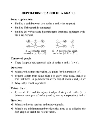
  • 1. DEPTH-FIRST SEARCH OF A GRAPH Some Applications: • Finding a path between two nodes x and y (an xy-path). • Finding if the graph is connected. • Finding cut-vertices and bicomponents (maximal subgraph with-out a cut-vertex). A B D C E F (i) A connected graph on nodes {A, B, ×××, F}. A B D C E F (ii) A disconnected graph on nodes {A, B, ×××, F}. Connected graph: • There is a path between each pair of nodes x and y (y ¹ x). Question: •? What are the simple (acyclic) DE-paths for the graph on left? •? If there is path from some node z to every other node, then is it true that there is a path between every pair of nodes x and y ¹ x? •? Why is this result important? Cut-vertex x: • Removal of x and its adjacent edges destroys all paths (³ 1) between some pair of nodes y and z; we say x separates y and z. Question: •? What are the cut-vertices in the above graphs. •? What is the minimum number edges that need to be added to the first graph so that it has no cut-vertex.
  • 2. 2.2 DEPTH-FIRST TREE Spanning Tree (of a connected graph): • Tree spanning all vertices (= n of them) of the graph. • Each spanning tree has n nodes and n - 1 links. Back-Edges and Cross-Edges (for a rooted spanning tree T): • Anon-tree edge is one of the following: - back-edge (x, y): joins x to ancestor y ¹ parent(x). - cross-edge (x, y): other non-tree edges. A B D C E F H G (i) Solid lines show a spannig tree A root B H C E F G D (ii) Dashed lines show back-edges; no cross-edges. Tree edges directed from parent to child. Depth-First Tree: • Arooted spanning tree with no cross-edges (as in (ii) above). Question: •? Show the back-edges and cross-edges if B is the root. Is this a depth-first tree (why)? Do the same for root = E and root = F. •? Show all spanning trees of the graph below (keep the nodes in the same relative positions). A B D C
  • 3. 2.3 VISITING EDGES IN A DEPTH-FIRST TRAVERSAL A B D C E F H G adjList(A) = áB, C, F, Hñ adjList(B) = áA, C, E, G, Dñ adjList(C) = áA, Bñ, adjList(D) = áB, Gñ adjList(E) = áB, Fñ, adjList(F) = áA, Eñ adjList(G) = áB, Dñ, adjList(H) = áAñ A 1, root 2 B H 8 3 C 4 E 5 F G 6 D 7 (ii) The dfTree, dfLabels, and back-edges. Order of Processing Links and Backtracking: StartNode = A. (A, B) tree-edge (G, B) 2nd visit (B, A) 2nd visit (G, D) tree-edge (B, C) tree-edge (D, B) back-edge (C, A) back-edge (D, G) 2nd visit (C, B) 2nd visit backtrack D®G backtrack C®B backtrack G®B (B, E) tree-edge (B, D) 2nd visit (E, B) 2nd visit backtrack B®A (E, F) tree-edge (A, C) 2nd visit (F, A) back-edge (A, F) 2nd visit (F, E) 2nd visit (A, H) tree-edge backtrack F®E (H, A) 2nd visit bacltrack E®B backtrack H®A (B, G) tree-edge backtrack A® Two Basic Operations: Move forward and backtrack. Question: •? Show the order of processing the links and backtracking if we reorder adjList(A) = áF, B, C, Hñ for the above graph.
  • 4. 2.4 USE OF STACK AND DEPTH-FIRST LABEL FOR DEPTH-FIRST TRAVERSAL A B D C E F H G adjList(A) = áB, C, F, Hñ adjList(B) = áA, C, E, G, Dñ adjList(C) = áA, Bñ, adjList(D) = áB, Gñ adjList(E) = áB, Fñ, adjList(F) = áA, Eñ adjList(G) = áB, Dñ, adjList(H) = áAñ A 1, root 2 B H 8 3 C 4 E 5 F G 6 D 7 (ii) The dfTree, dfLabels, and back-edges. Stack Node LastDf-or Link Label Processing áAñ A 0 ®1 dfLabel(A) = 1, nextNode = B = adjList(A, 0), nextToVisit(A) = 1¬0 (A, B) tree-edge, parent(B) = A, add B to stack áA, Bñ B 1 ®2 dfLabel(B) = 2, nextNode = A = adjList(B, 0), nextToVisit(B) = 1¬0 (B, A) second-visit, nextNode = C = adjList(B, 1), nextToVisit(B) = 2¬1 (B, C) tree-edge, parent(C) = B, add C to stack áA, B, Cñ C 2 ®3 dfLabel(C) = 3, nextNode = A = adjList(C, 0), nextToVisit(C) = 1¬0 (C, A) back-edge, nextNode = B = adjList(C, 1), nextToVisit(C) = 2¬1, (C, B) second-visit, backtrack áA, Bñ B nextNode = E = adjList(B, 2), nextToVisit(B) = 3¬2 (B, E) tree-edge, parent(E) = B, add E to stack áA, B, Eñ E 3 ®4 dfLabel(E) = 4, nextNode = B = adjList(E, 0), nextToVisit(E) = 1¬0 (E, B) second-visit, nextNnode = F = adjList(E, 1), nextToVisit(E) = 2¬1 (E, F) tree-edge, parent(F) = E = adjList(E, 1), nextToVisit(E) = 3¬2 ××× ××× ××× ×××
  • 5. 2.5 DATA-STRUCTURES IN DEPTH-FIRST TRAVERSAL ALGORITHM Array Data-Structures (each array-size = numNodes): dfLabels[i]: the depth-first label (³ 1) assigned to node i; each dfLabels[i] = 0, initially. nextToVisits[i]: nextToVisits[i] gives the position of the item in adjList of node i that is to be visited next from node i; each nextToVisit[i] = 0, initially; parents[i]: the parent of node i in depth-first tree; par-ents[ startNode] = startNode, initially. Additional Data-Structures: • lastDfLabel = 0, initially; it is incremented by one before assigning it to a node. • stack[0..numNodes-1]; it is initialized with the startNode and it contains the path in the depth-first tree from the root to the current node = top(stack). Notes: • You can add parent, dfLabel, and nextToVisit information in the structure GraphNode as shown below. typedef struct { int degree, *adjList, //arraySize = degree nextToVisit, //0<=nextToVisit<degree parent, dfLabel; } GraphNode; In that case, the next link to visit from node i is link (i, j), where j = nodes[i].adjList[nodes[i].nextToVisit]; otherwise, j = nodes[i].adjList[nextToVisit[i]].
  • 6. 2.6 PSEUDOCODE FOR DEPTH-FIRST TRAVERSAL ALGORITHM First Version: 1. Try to go down the tree (which is being created) from the current node x by choosing a link (x, y) in the graph from x to a node y not yet visited and adding the link (x, y) to the tree. 2. If there is no such node y, then backtrack to the parent of the current node, and stop when you backtrack from the startNode (= root of the tree). AMore Detailed Version (with parents[] and nextToVisit[]): 1. Initialize the arrays parents[] and nextToVisit[] as indicated in the previous page and let currentNode = startNode. 2. Search adjList[currentNode] from the position nextToVisit[cur-rentNode] onwards for a nextNode which is not yet visited, 3. [Move forward.] If (nextNode is found), then let parents[nextN-ode] = currentNode, update nextToVisit[currentNode], and cur-rentNode = nextNode. 4. [Backtrack.] If (no nextNode is found) then do the following: (i) If (currentNode = startNode) then stop. (ii) Otherwise backtrack, i.e., let currentNode = parents[cur-rentNode] and goto step (2).
  • 7. 2.7 DEPTH-FIRST TRAVERSAL ALGORITHM Algorithm DepthFirstTraverse: Input: A graph in adj-list form and a start-node. Output: A depth-first spanning tree for the connected component containing start-node. 1. Initialize lastDfLabel, the stack, and also the arrays dfLabels, parents, and nextToVisits as indicated in the previous page. 2. While (stack ¹ empty) do the following: (a) Let currentNode = top(stack) and if (dfLabels[currentNode] = 0) then update lastDfLabel and let dfLabels[currentNode] = lastDfLabel. (b) If (nextToVisit[currentNode] = degree[currentNode]) then backtrack by removing top of stack. (c) Otherwise, let nextNode = the node in position nextTo- Visit[currentNode] in adjList(currentNode), and update nextToVisit[currentNode]. Classify the link (currentNode, nextNode) as follows searching for a tree-edge (if any) from currentNode: (i) if (dfLabels[nextNode] = 0) then it is a tree-edge; let parent[nextNode] = currentNode, add nextNode to stack. (ii) if (dfLabels[nextNode] < dfLabels[currentNode]) then if (nextNode ¹ parents[currentNode]) then it is a back-edge and otherwise it is a second visit of tree-edge. (iii) Otherwise, it is a second visit to a back-edge. Note: We merged old (c)-(d), eliminated all goto’s and putting (c)-(d) in a loop, and split d(ii) into d(ii)-(iii). Also, added an if-part in (a).
  • 8. 2.8 EXERCISE 1. How many times a link (x, y) is visited and when? 2. What is the total number of back-edges? 3. How many tree-edges and back-edges are there at a node x? 4. How many times does a node x enter the stack and when? 5. How many times do we backtrack to a node x? How many times do we backtrack from a node x and when? 6. Shown below is a graph and a depth-first tree for startNode = A. A B D C E F H G (i) A graph. A root B H C E F G D (ii) A depth-first tree. (a) Show all possible orderings of the adjacency list of A which will give this tree when we apply the depth-first tra-versal algorithm. Do the same for node B, keeping startN-ode = A. (b) Give the total number of ways of ordering the various adjacency lists which will give the above depth-first tree. (c) Arrange all adjacency-lists in such a way that at each node x, the tree-edges from x to its children are visited first, then the back-edges from x (if any, to its ancestors), next the second-visit of tree-edge connecting x to its parent (if any), and finally the second-visit of back-edges to x (if any, from its descendants).
  • 9. 2.9 7. How do you distinguish a second-visit to a tree edge vs. a sec-ond- visit to a backedge? 8. For each edge processed in the table on page 3, show the asso-ciated step of the algorithm on page 7 that is used for it. 9. Show the modifications to the delth-first traversal algorithm to compute maxDfLabel(x) = max {dfLabel(y): y = x or a descendant of x} for each node x. Use the depth-first tree above to explain how this works. How can you compute the size of the subtree at x using maxDfLabel(x)? 10. Is it true that the nodes in the subtree at x of a depth-first tree consists of all nodes that can be reached from x without using any of the other nodes on the path from root to x?
  • 10. 2.10 A RECURSIVE VERSION OF DF-TRAVERSAL Notes: • Backtracking corresponds to return from the recursion. • The lastDfLabel and the dfLabels-array can be static in DF-TRAVERSAL; the nextToVisit-array is not used. • The recursive-call at x creates the subtree of df-tree at x as we build the df-tree via child-pointers, etc. Algorithm DF-TRAVERSAL(currNode): //first call: currNode = s Input: A graph in adj-List form and a start-node s. Output: The df-tree, with root = s. 1. [Create df-tree node.] Create currTreeNode in df-tree for currN-ode. If (lastDfLabel = 0), then initialize dfLabel(x) = 0 for each x and let parent(currTreeNode) = currTreeNode. Now, let dfLa-bel( currNode) = lastDfLabel = lastDfLabel + 1. 2. For (each node x in adjList(currNode)) do the following: If (dfLabel(x) = 0) then add the root-node (which corre-sponds to x) of the subtree returned by DF-SEARCH(x) as the next child of currTreeNode. 3. Return(currTreeNode). Complexity: O(|V| + |E|) = O(|E|) for a connected G. • An edge (x, y) is examined at most once in each direction. • Aconstant amount of work per node x (assigning dfLabel(x), adding x to the df-tree, and backtracking from x).
  • 11. 2.11 ILLUSTRATION OF THE RECURSIVE DF-TRAVERSAL L A K A/1 B J B/2 J/3 K/4 L/5 DF-TRAVERSAL(A) parent(A) = A dfLabel(A) = 1 = lastDfLabel parent(B) = A DF-TRAVERSAL(B) dfLabel(B) = 2 = lastDfLabel parent(J) = A DF-TRAVERSAL(J) dfLabel(J) = 3 = lastDfLabel parent(K) = J DF-TRAVERSAL(K) dfLabel(K) = 4 = lastDfLabel parent(L) = A DF-TRAVERSAL(L) dfLabel(L) = 5 = lastDfLabel • #(calls to DF-TRAVERSAL) = #(nodes in df-tree) = #(nodes in graph), if G is connected. • #(direct calls from DF-TRAVERSAL(x)) = #(children x).
  • 12. 2.12 A SAMPLE OUTPUT OF DF-TRAVERSAL PROGRAM L 4 3 K A 0 B 1 2 J Input Graph: numNodes = 5 0 (4): 1 2 3 4 1 (1): 0 2 (2): 0 3 3 (2): 0 2 4 (1): 0 ------------------------------ startNode = 0, dflabel(0) = 1 processing (0,1): tree-edge, dfLabel(1) = 2 processing (1,0): tree-edge 2nd-visit backtracking 1 -> 0 processing (0,2): tree-edge, dfLabel(2) = 3 processing (2,0): tree-edge 2nd-visit processing (2,3): tree-edge, dfLabel(3) = 4 processing (3,0): back-edge processing (3,2): tree-edge 2nd-visit backtracking 3 -> 2 backtracking 2 -> 0 processing (0,3): back-edge 2nd-visit processing (0,4): tree-edge, dfLabel(4) = 5 processing (4,0): tree-edge 2nd-visit backtracking 4 -> 0 ------------------------------ PROGRAMMING EXERCISE 1. Create a function depthFirstTraverse(int startNode). It should produce output as indicated above. Use an auxiliary function readGraph (input file should be in the same form as for a digraph using adjacency-lists), which should output the graph read. keep the adjacency lists sorted in increasing order. Show the output for the 8 node graph on page 2.2 with startNode B (= 1).
  • 13. 2.13 NODE-STRUCTURE FOR AN ORDERED-TREE • The parent-links alone do not allow us to traverse the df-tree from the root (= startNode of depth-first traversal). • Since the number of children of a node is known ahead of time, the children are kept in a linked-list. • The lastChild pointer helps addition of a child and firstChild pointer accessing the children. typedef struct TreeNode { int node, numChildren; struct TreeNode *parent, *leftBroth, *rightBroth, *firstChild, *lastChild; } TreeNode; parent(x) leftBroth(x) x rightBroth(x) firstChild(x) lastChild(x) Example. Null-pointers not shown; firstChild(J) = lastChild(J). The nodes are numbered 0, 1, ××× in alpabetical order. A/0; 3 B/1; 0 J/2; 1 L/4; 0 K/3; 0 firstChild lastChild parent rightBroth leftBroth
  • 14. 2.14 ALL ACYCLIC PATHS IN A GRAPH FROM A START-NODE Example. Shown below is a graph and the tree of all acyclic paths from a. a b d c e (i) A graph G. a b c d e d c e d b c c b e e d b c c b (ii) The tree of acyclic paths from a in G. Some Properties of this Tree (startNode = s): • Anode x appears in the tree as many times as the number of acyclic paths to x from s. • We can find all cycles (without repetition of nodes) at a node s from these paths: - Combine an sx-path with the edge (s, x), if exists. - Each cycle is obtained twice in this process, once in each direction. • We can find if there is a Hamiltonian cycle (cycle containing all nodes exactly once). Note: • To deremine all acyclic paths from startNode, use the depth-first traversal with the change: reset nextToVisit[i] = 0 = dfLabel[i] in backtrack from node i.
  • 15. 2.15 OBJECT-REGION IN A BINARY-IMAGE Binary-image: • Anm´narray, where a pixel pij = 1 (shown below as a shaded square) represents a part of an object in the image; a pixel pij = 0 represents a part of the background. A 6´6 binary image. Adjacent Pixels: • Two 1-pixels are adjacent if they share an edge. • Two 0-pixels are adjacent if they share a corner or an edge. pi-1, j pi, j-1 pi, j pi, j+1 pi+1, j At most 4 neighbors of an 1-pixel pij . pi-1, j pi, j-1 pi, j pi, j+1 pi+1, j At most 8 neighbors of a 0-pixel pij . Image-object: A maximal set of connected 1-pixels pij . Example. The above image has 2 objects of sizes 7 and 4 and two background regions of sizes 1 and 24. Question: Give a 5´5 image with maximum number of objects.
  • 16. 2.16 OBJECT DETERMINATION BY DF-TRAVERSAL Order of Visit of Neighbors of 1-pixel pij (if present): (1) pi, j+1 (E-neighbor) (3) pi, j-1 (W-neighbor) (2) pi-1, j (N-neighbor) (4) pi+1, j (S-neighbor) Additional Backtracking Rule: • If we reach a 0-pixel, we immediately backtrack. Example. Shown below is the depth-first labeling of the pixels vis-ited starting at the position labeled 1. All neighboring 0-pixels of the region R containing the start-pixel are also visited. The total number of visits to those 0-pixels is at most 2(|R| + 1) - why? 7 5 6 9 3 4 1 2 14 8 10 12 11 13 15 18 16 17 start-pixel 1 2 E 3 N 4 E 5 N 6 E 7 N 8 W 9 W 8 N W 10 W 11 S E W 12 S 13 14 S 15 E W 13 16 S E 17 W 18 The dashed lines indicate neighbor that are visited but are not in the current region. These nodes appear as many times as they are visited, each time causing an immediate backtracking; both nodes 8 and 13 appear here twice.
  • 17. 2.17 INTERNAL AND EXTERNAL BOUNDARIES OF AN OBJECT Non-Boundary (internal) Pixel p of An Object: • Completely surrounded by 8-neighbor object pixels. p Two Types of Background Pixels: • 0-regions are based on 8-neighbors. • External regions: 0-regions which contain at least one pixel in the first or last row or first or last column. • Holes: other 0-regions completely surrrounded by object pixels; does not contain pixels from first (last) row or column. ´ ´ ´ ´ ´ ´ ´ ´ ´ ´ ´ ´ Two holes of sizes 2 and 3. Two external regions of sizes 3 and 15. Internal pixel of the object Only external boundary pixels Only internal boundary pixels ´ Both internal and external boundary pixels Two Types of Boundary (non-internal) Pixels: • Internal boundary: Objects pixels adjacent to holes (based on 8-neighbors). • External boundary: Object pixels adjacent (based on 8-neigh-bors) to external regions or in the first (last) row or column. Question: Show the boundary and internal pixels if the pixel p5,4 above were a 0-pixel (merging two holes into one),
  • 18. 2.18 VISITING A MAZE OR EXTERNAL BOUNDARY OF AN OBJECT Strategy: • Keep to the right, starting at a southmost pixel of maze or object. • Assume that we arrived at the start-position with a north-move (thus, attempt to go east first at start-position). Start-point Part of the move sequence visiting a maze. The trail of "return visits" parts are shown in bold. The move sequence visiting the external boundary of an object. Question: Show the move sequence if we start at pixel p3,3.
  • 19. 2.19 OBJECT SIMPLIFICATION BY FILLING UP HOLES IN THE OBJECT An image with three objects. The largest object contains two holes and one of the objects is placed in one of those holes. The non-boundary pixels of this object are shown in light shade. • • • External Regions: • The 0-regions which contain at least one 0-pixel from any of top/bottom rows and leftmost/rightmost columns. Holes: These are 0-regions other than the external regions. After filling-in the two holes in the largest object. This swallows the third object in one of those holes. • • Questions: 1? Show df-labels of pixels in the 0-region in the top image starting at p1,1 (top-left pixel); do not label 1-pixels that may be visited. 2? Give a psuedocode to detect the pixels in the holes of an object. What is the computational complexity? 3? Mark successively as 1, 2, ××× for the first visit to the 1-pixels starting at the southmost pixel p11,10 ( p1,1 = the top-left pixel) of the largest object in the top figure and using the rule "keep to the right". The next pixel visited would be p10,10. (Note: there is no backtracking here, and some pixel may be visited more than once. As usual, assume we arrived at p11,10 by going north.)
  • 20. 2.20 TREE OF SHORTEST-PATHS IN DIGRAPHS C 3 1 D 2 1 5 A 2 B 1 E 1 5 A digraph ®G with each c(x, y) ³ 0. Start-node s = A. • • A 2 B 5 C 10 D E 3 C 8 D 13 D 1 E 1 C 6 7 B D 11 • Bold links show the tree of shortest-paths to various nodes. The tree of acyclic paths from A; shown next to each node is the length of the path from root = A. Some Important Observations: • Any subpath of a shortest path is a shortest path. • The shortest paths from a startNode to other nodes can be chosen so that they form a tree. Question: •? What are some minimum changes to the link-costs that will make áA, B, E, Cñ the shortest AC-path? •? Show the new tree of acyclic paths ad the shortest paths from startNode = A after adding the link (D, B) with cost 1. •? Also show the tree of acyclic paths and the shortest paths from the startNode = D.
  • 21. 2.21 ILLUSTRATION OF DIJKSTRA’S SHORTEST-PATH ALGORITHM C 3 1 D 1 1 A 2 B 2 5 1 E 1 5 d(x) = length of best path known to x from the startNode = A. A node is closed if shortest path to it known. A node is OPEN if a path to it known, but no shortest path is known. • • • "?,?" indicates unknown values, "×××" indicates no changes, and "-" indicates path-length not computed (would not have changed any way). Open Node Links d(x) and parent(x) Nodes Closed processed A B C D E {A} Æ 0, A ?, ? ?, ? ?, ? ?, ? {B} A (A, B) 2, A {B, D} (A, D) 1, A {B, D, E} (A,E) 1, A {B, E} D (D, A) - (D, B) ××× {B, C} E (E, C) 6, E {C} B (B, C) 5, B (B, E) - Æ C (C, B) - (C, D) - Question: •? List all paths from A that are looked at (length computed) above. •? When do we look at a link (x, y)? How many times do we look at a link (x, y)? •? What might happen if some c(x, y) < 0?
  • 22. 2.22 DIJKSTRA’S ALGORITHM Terminology (OPENÇCLOSED = Æ): CLOSED = {x: p m(s, x) is known}. OPEN = {x: some p (s, x) is known but x ÏCLOSED}. Algorithm DIJKSTRA (shortest paths from s): Input: AdjList(x) for each node x in ®G , each c(x, y) ³ 0, a start-node s, and possibly a goal-node g. Output: A shortest sg-path (or sx-path for each x reachable from s). 1. [Initialize.] d(s) = 0, mark s OPEN, parent(s) = s (or NULL), and all other nodes are unmarked. 2. [Choose a new closing-node.] If (no OPEN nodes), then there is no sg-path and stop. Otherwise, choose an OPEN node x with the smallest d(×), with preference for x = g. If x = g or all but one node are closed, then stop. 3. [Close x and Expand p m(s, x).] Mark x CLOSED and for (each y ÎadjList(x) and y not marked CLOSED) do: if (y not marked OPEN or d(x)+c(x, y) < d(y)) then let par-ent( y) = x, d(y) = d(x) + c(x, y), and mark y OPEN. 4. Go to step (2). Complexity: O(N2). • A node x is marked CLOSED at most once and hence a link (x, y) is processed at most once. • Each iteration of steps (2) and (3) takes O(N) time.