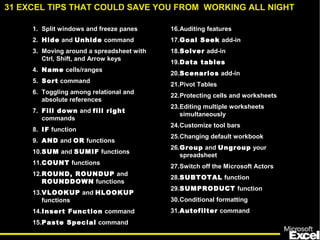
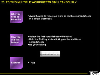
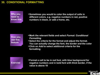
SlideShare a Scribd company logo
1 of 42
31 Excel
Tips
That Could Save
You from Working
All Night
What is it: The following material was developed for the Seoul office training
program.
Target audience: 1st year associates and business analysts, although there
is nothing wrong doing this training as well with EMs and APs.
Duration: 3-4 hours to walk through the explanations and give everyone a
chance to actually practice.
Faculty: SEO did it with 2 MGMs, which was extremely powerful, since the
seniors showed that they can do and therefore they can expect their team
members to do the same.
Final comment: The original material was not intended for self-study
purposes and therefore may be a little be too brief and cryptic in some cases. In
case you have any improvement ideas please feel free to e-mail them to the
authors.
INTRODUCTORY NOTE
1. Split windows and freeze panes
2. Hide and Unhide command
3. Moving around a spreadsheet with
Ctrl, Shift, and Arrow keys
4. Name cells/ranges
5. Sort command
6. Toggling among relational and
absolute references
7. Fill down and fill right
commands
8. IF function
9. AND and OR functions
10.SUM and SUMIF functions
11.COUNT functions
12.ROUND, ROUNDUP and
ROUNDDOWN functions
13.VLOOKUP and HLOOKUP
functions
14.Insert Function command
15.Paste Special command
16.Auditing features
17.Goal Seek add-in
18.Solver add-in
19.Data tables
20.Scenarios add-in
21.Pivot Tables
22.Protecting cells and worksheets
23.Editing multiple worksheets
simultaneously
24.Customize tool bars
25.Changing default workbook
26.Group and Ungroup your
spreadsheet
27.Switch off the Microsoft Actors
28.SUBTOTAL function
29.SUMPRODUCT function
30.Conditional formatting
31.Autofilter command
31 EXCEL TIPS THAT COULD SAVE YOU FROM WORKING ALL NIGHT
•Splitting a window allows you to work on multiple parts
of a large spreadsheet simultaneously
•Freezing the pane allows you to always keep one part of
the spreadsheet (e.g., column or row labels) visible
How you
use this
feature
•Drag the split horizontal and split vertical icons to the
desires positions
•Click on the freeze pane icon from the tool bar to freeze
the panes
Exercise
•Split the screen so that:
–The row with column labels shows up in the top pane
–The column with store names show up in the left pane
•Freeze the panes
Freeze pane icon
Split screen icons
1. SPLIT WINDOWS AND FREEZE PANES
Why you
need to
know this
•Allows you hide and unhide particular rows or
columns
–Simplifies working with the spreadsheet
–Prevent certain information from being seen
•Select the row(s) or column(s) to be
hidden/unhidden
•Select Format : Row : Hide/Unhide or Format :
Column : Hide/Unhide
•Hide the Avg Sale/Ticket column
2. HIDE AND UNHIDE COMMAND
How you
use this
feature
Exercise
Why you
need to
know this
•Save you lots of time
•Move the first or last cell of a contiguous data block
without scrolling
•Ctrl-Arrow : Move to the first/last data cell in the arrow
direction
•Ctrl-Shift-Arrow : Selects the cells between the current
cell and the first/last data cell
•Select all cells with data using the Ctrl, Shift, and Arrow
keys
3. MOVING AROUND A SPREADSHEET WITH CTRL, SHIFT, AND ARROW
KEYS
How you
use this
feature
Exercise
Why you
need to
know this
•Allows specific cells or cell ranges to be referred to by
name
•Allows you to write equations such as = Quantity*Cost
instead of =$B$12*$C$4
•Select the cell or cell range
•Select Insert : Name : Define from the menu bar
•Define cells A2:A125 as “Sequence”
4. NAME CELLS/RANGES
How you
use this
feature
Exercise
Why you
need to
know this
•Correctly sorting a series of rows or columns
without disassociating the data is critical to many
modeling efforts
•Select all cells in the data range to be sorted
•Select Data : Sort from the menu bar
•Sort the dataset by ascending store name
5. SORT COMMAND
How you
use this
feature
Exercise
Why you
need to
know this
•Saves you lots of time
•F4 key toggles through the different options
6. TOGGLING AMONG RELATIONAL AND ABSOLUTE REFERENCES
How you
use this
feature
Why you
need to
know this
•Saves you lots of time
•Allows for copying of cell content to contiguous cells
with a single keystroke
•Select the cell with the content to be copied and drag to
select the cells to which the content should be copied
•Ctrl-R to fill right
•Ctrl-D to fill down
•Double-check your formulas for absolute vs. relative
references!!
•Calculate the total daily sales for each store
How you
use this
feature
Exercise
Caution!!
7. FILL DOWN AND FILL RIGHT COMMANDS
Why you
need to
know this
•Conditional comparisons are used in virtually all
spreadsheets
•Knowing how to use IF in a nested manner and in
combination with other functions will save hours of time
•IF(Comparison,TrueAction,FalseAction)
•IF(Comparison,TrueAction,) ==> Cell shows 0 if
condition is false
•IF(Comparison,TrueAction,””) ==> Cell shows blank if
condition is false
•Create a “Seoul” variable
–1 if the store is in Seoul
–0 if the store is in other places
8. IF FUNCTION
How you
use this
feature
Exercise
Why you
need to
know this
•Used with the IF function to enable more complicated
logical comparisons
•AND(Comparison 1,Comparison2,Comparison3,…)
•OR(Comparison 1,Comparison2, Comparison3,…)
•Create a variable that calculates daily sales per pyung
only for:
–KFC stores in Seoul with size larger than 50 pyung
–All BK stores
9. AND AND OR FUNCTIONS
How you
use this
feature
Exercise
Why you
need to
know this
•SUM is used in virtually all spreadsheets
•SUMIF can save lots of time in most spreadsheets if you
know how to use the function
•SUM(Range1,Range2,Value1,…)
•SUMIF(Range,”Comparison”,SumRange)
–If a SumRange IS NOT specified, SUMIF sums the cells
meeting the Comparison criteria in the specified Range
–If a SumRange IS specified, SUMIF sums the cells in
SumRange where the corresponding cells in Range
meets the Comparison criteria
•NOTE: The “” signs must be used for the Comparison
value
•Calculate the total store space for stores larger than 50
pyungs
•Calculate the total daily sales for all stores larger than 50
pyungs
10. SUM AND SUMIF FUNCTIONS
How you
use this
feature
Exercise
Why you
need to
know this
•Prevents you from wasting time counting items manually
or creating dummy variables to count such items
•COUNT(Range1,Range2,Value1,...) ==> count the number
of cells containing numbers
•COUNTA(Range1,Range2,Value1,...) ==> count the
number of non-empty cells
•COUNTBLANK(Range) ==> count the number of empty
cells in the range
•COUNTIF(Range,”Criteria”) ==> count the number of
cells in the Range containing the Criteria. NOTE: The “”
signs must be used for the Criteria value
•Calculate the number of KFC stores in the dataset
11. COUNT FUNCTIONS
How you
use this
feature
Exercise
Why you
need to
know this
•Many situations exist when you need to have exact
numbers instead of various fractions in your calculations
(e.g., there cannot be 536.235 bank branches)
•ROUND(Number,Digits) ==> Round the number (or cell)
to the specified number of digits
–If Digit = 0, then Number is rounded to nearest integer
–If Digit > 0, then Number is rounded to the specified
number of decimal places
–If Digit < 0, then Number is rounded to the specified
number of digits left of the decimal place
•ROUNDDOWN(Number,Digits) and
ROUNDUP(Number,Digits) work the same way as
ROUND, but the direction of rounding is specified by the
function
•Calculate a rounded Avg Sale/Ticket variable, rounding
to the nearest 10 Won
12. ROUND, ROUNDUP AND ROUNDDOWN FUNCTIONS
How you
use this
feature
Exercise
Why you
need to
know this
•Allows you to automatically lookup a particular cell of
data from a larger data range. This is especially useful
when you have
–A large data section that contains information for
multiple records somewhere on the spreadsheet (e.g., a
small database)
–A calculation area somewhere else, and you need to
refer to some specific data elements for specific
records
13. VLOOKUP AND HLOOKUP FUNCTIONS (CONTINUED)
Why you
need to
know this
• VLOOKUP and HLOOKUP allows you to find a specific cell of data
in a larger data range
– Use VLOOKUP when each row contains a separate record and
the associated columns contain data for that one record
– Use HLOOKUP when each column contains a separate record
• VLOOKUP(SearchValue,Range,ColumnNumber,Error) ==> look
for a value in the row specified by SearchValue and the column
specified by ColumnNumber
– SearchValue indicates the “match key” (i.e., find the row that
contains the SearchValue in the first column)
– Range specifies the cells containing the data
– ColumnNumber specifies the column that contains the data
element you want
– Error determines what happens when Excel does not find the
exact SearchValue you want. FALSE leads Excel to display a
#N/A when an exact match cannot be found. TRUE leads Excel
to display the next smaller value than SearchValue
• HLOOKUP(SearchValue,Range,RowNumber,Error) ==> look for a
value in the column specified by SearchValue and the row
specified by RowNumber
NOTE: The 1st column of data must be sorted in ascending order
when using VLOOKUP, and the 1st row of data must be sorted if
using HLOOKUP
13. VLOOKUP AND HLOOKUP FUNCTIONS (CONTINUED)
How you
use this
feature
•Define a name for the cells containing the data and use
that name as the Range. Do not include the row/column
label in the named range because this would break the
ascending sort rule above.
•Insert an extra row above your column label to number
the columns
•Use VLOOKUP to find out how many seats are in the
Duksung store? How passers-by for the store?
13. VLOOKUP AND HLOOKUP FUNCTIONS
Exercise
Tip
Define a
name for
cells in your
data Range
Number the
columns to
easily check
your
formulas
Need to sort in
ascending order
for VLOOKUP
function to work
properly
•What do you do if you do not know what functions are
available or how to enter the arguments for a function?
•Select the cell
•Select Insert : Function from the menu bar
•Calculate the median daily ticket count for all the stores
14. INSERT FUNCTION COMMAND
How you
use this
feature
Exercise
Why you
need to
know this
• Saves you lots of time
– Retyping formulas
– Converts formulas into values
– Reformatting cells
– Transposing cells (i.e., convert row-entered data blocks into
column-entered ones)
• Convert the Rounded Avg Sale/Ticket calculations into values
(i.e., get rid of the formulas)
• Copy and paste the entire dataset into a new spreadsheet in
transposed manner
• Copy the cells of interest
• Place the cursor where you want to past the information
• Select Edit : Paste Special from the menu bar
• Select the appropriate options from the dialog box that appears
15. PASTE SPECIAL COMMAND
How you
use this
feature
Exercise
Why you
need to
know this
•Quickly find the cells referenced by a formula and/or
quickly find which cells reference a particular cell of
interest
•Select View : Toolbars : Customize from the menu bar.
Check the Auditing box from the Toolbars tab
•Click on the cell of interest
•Select the Trace Precedents or Trace Dependents icon
from the Auditing Toolbar
•Find the cells that references the Daily Ticket Count for
the Ansan store
16. AUDITING FEATURES
How you
use this
feature
Exercise
Why you
need to
know this
•Easily find what one input variable needs to be to
achieve some desired result in a calculation
•Select the calculated cell
•Select Tools : Goal Seek from the menu bar
•Enter the desired resulting calculation into the “To
Value” form in the dialog that appears
•Enter the input cell in the “By changing cell:” form
•How many additional daily tickets would the Achasan
store need to have a total daily sales of 2,000,000 Won?
17. GOAL SEEK ADD-IN
How you
use this
feature
Exercise
Why you
need to
know this
•Allows you to use linear programming to find the optimal
inputs to achieve some desired calculational result (e.g.,
maximize revenues by increasing daily tickets,
increasing store size, average sale/ticket, etc.
simultaneously)
•Use Solver instead of Goal Seek when:
–You need to place constraints on the input variable
(e.g., cannot open a store for more than 24 hours a day)
–More than 1 input variables are involved
–You want to minimize or maximize the resulting
calculation in addition to just setting the calculation to
a predetermined value
18. SOLVER ADD-IN (CONTINUED)
Why you
need to
know this
•Select the final calculated cell, then select Tools : Solver
from the menu bar
•Select what you want to do from the “Equal to” section
(I.e., maximize, minimize, or set to a specific value)
•Reference the input cells (note, separate cells by using a
comma or “:” if cells are contiguous
•If the input values have constraints, click on Add to enter
the constraints
•Click on Solve
•What is the maximum daily sales per pyung for the
Ansan store if:
–The store can be opened a maximum of 18 hours/ day,
7 days/week
–Store size can expanded up to a maximum of 87 pyung
How you
use this
feature
Exercise
18. SOLVER ADD-IN
• Simplest way to run sensitivity analyses
• Input the values you want to test for a particular variable on
separate rows (e.g., A6:A13)
• In the cell above and to the right of the first sensitivity value,
reference the final result of your calculations (e.g., A5 = C3)
• Select the cells containing the calculation and input variables
(e.g., A5:B13)
• Select Data : Tables from the menu bar
• Input the cell referenced by the formula in the“Column input
cell”(e.g., A2). This example uses in “Column input cell”
because the value to test in the sensitivity analysis are arranged
in a single column
19. DATA TABLES COMMAND (CONTINUED)
How you
use this
feature
Why you
need to
know this
•What daily total sales would the Achasan store have its
daily ticket counts ranged from 400 to 600 each day (in
increments of 50)?
19. DATA TABLES COMMAND
Exercise
• You’ve created a model and need to run various scenarios. Then
use the scenario function under the tools menu. Keeps your
inputs and outputs from the model nicely together
• Assign names to the excel cells that act as input parameters for
your model
• Start the scenario function by selecting Tools : Scenarios from
the menu bar.
• Click Add to enter your first scenario
– Create a name
– Select ALL cells that will be your input to the model.
• Assign the desired scenario value to each input parameter.
• Add more scenarios as needed
• When finished click on summary and select scenario summary
(the pivot table is not so helpful)
20. SCENARIOS ADD-IN
How you
use this
feature
Why you
need to
know this
Objective:
You want to build a simple model to understand under which
scenarios Airbus should build the A3XX a next generation
super large airplane with more than 600 seats
Simple model:
Profit = number of planes sold x price x margin -
development cost
Scenarios Worst case Realistic Best case
No. of planes 200 350 500
Price (million. USD) 120 130 150
Margin 20% 25% 30%
R&D 13 billion USD 12 billion USD 11 billion USD
20. SCENARIOS ADD-IN (SIMPLE EXAMPLE)
• Most powerful tool to arrange huge amounts of data in a more
structured way than pure sorting. In particular helpful to run
quick sums, averages, distributions, etc. in combination with a
structure criteria, e.g. total number and average sales per store
size band
• Select Data: PivotTable Report…
Step 1: Microsoft
Excel list
Step 2: Select
the relevant
data area
• Step 3: Drag and drop data elements
on row and column (this is your table
structure), the data you want to
analyze on the data area
• Step 4: Just press Finish
21. PIVOT TABLES
How you
use this
feature
Why you
need to
know this
•Draw a distribution chart for the number of stores per
size in pyung bucketed each 10 pyung wide
•Arrange the store distribution by store size (each 10
pyung) and daily tickets (each 100 tickets) and show the
number of stores per each category
21. PIVOT TABLES
Exercise
• Sometimes you want to give your Excel file to someone else and
prevent them from changing the formulas for seeing some hidden
cells
• Protecting a spreadsheet or workbook involves two steps
– Designating which cells to be locked or hidden
– Protecting the spreadsheet or workbook
• Note several weird peculiarities:
– The default for all cells in a spreadsheet if LOCKED. So if you
want the receiver of your worksheet to change the content of a
cell, unlock the cell before protecting the spreadsheet
– The formulas in a cell can be seen even if the spreadsheet is
lock -- UNLESS you hide that cell before protecting the
spreadsheet
• To lock/unlock and hide/unhide a cell, select the cell(s) and select
Format : Cell. Select the Protection tab when the dialog box
appears
• To protect/unprotect a spreadsheet, select Tools : Protection :
Protect Sheet
• Protect the dataset spreadsheet
– Allow the user to change the data
– Lock and hide the formulas you entered
22. PROTECTING CELLS AND WORKSHEETS
How you
use this
feature
Exercise
Why you
need to
know this
•Avoid having to redo your work on multiple spreadsheets
in a single workbook
•Select the first spreadsheet to be edited
•Hold the Ctrl key while clicking on the additional
spreadsheets
•Do your editing
•Try it
23. EDITING MULTIPLE WORKSHEETS SIMULTANEOUSLY
How you
use this
feature
Exercise
Why you
need to
know this
•How many icons on the tool bar to you use regularly?
•How often do you have to use the menu bar or mouse to
do something you wish were accessible with a single
click?
•Select View : Toolbars : Customize
•Click on the Commands tab
•Drag items on and off the toolbar as you wish
•Modify your toolbar as desired
24. CUSTOMIZE TOOL BARS
How you
use this
feature
Exercise
Why you
need to
know this
•How often do you use the menu bar to change the normal
font or number formats?
•You can create the basic number and font formats you
use regularly, save it as a template, and have Excel use
that template every time you create a new workbook
•Create a workbook with the formatting you use regularly
and save it under the name “Book” and Template format
•Move the “Book” template to the Microsoft Office :
Office : Xlstart folder
•Create your default workbook
How you
use this
feature
Exercise
25. CHANGING DEFAULT WORKBOOK
Why you
need to
know this
•How often would you like to hide or unhide parts of a
complex spreadsheet?
•If your answer is “very often”. You will like to
group/ungroup function instead of the hide/unhide
command, since you will be able to toggle between
hidden or displayed columns or rows.
•Mark the row or column that you would like to “fold”, I.e.
hide for the moment.
•Click on Data: Group and Outline: Group
•To “fold” click now on the “minus” sign outside of your
column or row
•You may also group or ungroup hierarchically
•Group some parts in your spreadsheet
•Also try to remove the grouping
•Use the two “arrow” buttons, which you find on the pivot
table toolbar (right click on any toolbar and select
PivotTable)
26. GROUP/UNGROUP PARTS OF SPREADSHEETS
Exercise
Tip
How you
use this
feature
Why you
need to
know this
•Also find the Microsoft Actors more disturbing than
helpful?
•Always popping up at the wrong moment
•Start the Windows Explorer
•Go to the directory Program Files: Microsoft Office:
Office: Actors
•Rename the directory “Actors” to “Dead Actors”
•Try to eliminate the Actors
27. SWITCH OFF THE MICROSOFT ACTORS
Exercise
How you
use this
feature
Why you
need to
know this
•Want to add lines with subtotals in your P&L or balance
sheet, but still need to run the total over all numbers?
Don’t want to get confused with nested subtotals and
totals in your spreadsheet?
•Instead of ‘=sum(range)’ add ‘=subtotal(9, range)’ where
you need a subtotal or total.
•You may nest this function as you like. Excel keeps track
of everything
•Create a simple column with various numbers
•Add various subtotals running over various parts of your
spreadsheet and finally over the whole column
Exercise
How you
use this
feature
28. SUBTOTALS AND TOTALS
Why you
need to
know this
•If you need to multiply two column and need the sum of
the multiplication, sumproduct comes easy.
•Insert =sumproduct(range1, range2)
•Multiply two columns or rows and get the sum of it
28. SUMPRODUCT FUNCTION
Exercise
How you
use this
feature
Why you
need to
know this
•Of course you can create your own discounting table and
then calculate the NPV of your cash flow series or just
use the NPV function
•Insert =NPV(discount rate, cash flow numbers, ...)
•The discount rate is in percent
•The cash flow numbers are either an array or individual
numbers in individual cells
•Attention: The first cash flow number is in period 1, e.g.
the end of the period. If you have for example an initial
investment in period 0, just type =NPV(…)+period 0
payment in your calculation
•Create a list of random cash flows and calculate the NPV
with the NPV function
29. NPV FUNCTION
Exercise
How you
use this
feature
Why you
need to
know this
•Sometimes you would to color the output of cells in
different colors, e.g. negative numbers in red, positive
numbers in black, or add a frame, etc.
•Mark the relevant fields and select Format: Conditional
Formatting
•Select the criteria for the format and adjust the format.
You can actually change the font, the border and the color
•Click on Add to select additional criteria for the
formatting
•Format a cell to be in red font, with blue background for
negative numbers and in bold font with thick border, if the
value is above 10
30. CONDITIONAL FORMATTING
Exercise
How you
use this
feature
Why you
need to
know this
•You have a huge pile of data and quickly want to find
some specific information, e.g. all sets that meet a criteria
or the top 10 items etc.
•Click into your table or better mark the data area and
select Data: Filter: Autofilter
•Using the drop-down boxes per item allows you to
display only specific filtered information
•Selecting multiple matches (up to 3 maximum with
autofilter) you can narrow down your search
•Or add your own criteria for filtering by clicking on the
custom criteria
•Find the stores who belong to the top 10% in terms of
average sales per ticket AND the top 10 in terms of store
size in pyung
31. AUTOFILTER COMMAND
Exercise
How you
use this
feature
Why you
need to
know this

More Related Content

What's hot (17)

Excel tips
Excel tipsExcel tips
Excel tips
 
Excel Tips in computers
Excel Tips in computersExcel Tips in computers
Excel Tips in computers
 
35 Useful Excel Tips
35 Useful Excel Tips35 Useful Excel Tips
35 Useful Excel Tips
 
Excel useful tips
Excel useful tipsExcel useful tips
Excel useful tips
 
Excel tips
Excel tipsExcel tips
Excel tips
 
Excel useful tips
Excel useful tipsExcel useful tips
Excel useful tips
 
Excel useful tips
Excel useful tipsExcel useful tips
Excel useful tips
 
Excel Tips
Excel TipsExcel Tips
Excel Tips
 
Excel Tips
Excel TipsExcel Tips
Excel Tips
 
Excel Tips
Excel TipsExcel Tips
Excel Tips
 
Excel tips 172
Excel tips 172Excel tips 172
Excel tips 172
 
Excel tips
Excel tipsExcel tips
Excel tips
 
Excel Tips
Excel TipsExcel Tips
Excel Tips
 
Excel Tips
Excel TipsExcel Tips
Excel Tips
 
Excel Tips
Excel TipsExcel Tips
Excel Tips
 
Microsoft Excel Tips
Microsoft Excel TipsMicrosoft Excel Tips
Microsoft Excel Tips
 
Excel Useful Tips
Excel Useful TipsExcel Useful Tips
Excel Useful Tips
 

Viewers also liked (18)

METACOGNICIÓN
METACOGNICIÓN METACOGNICIÓN
METACOGNICIÓN
 
Harry Potter Student Personas
Harry Potter Student PersonasHarry Potter Student Personas
Harry Potter Student Personas
 
1
11
1
 
Edted - Novas oportunidades de negócios com as Redes Sociais
Edted - Novas oportunidades de negócios com as Redes SociaisEdted - Novas oportunidades de negócios com as Redes Sociais
Edted - Novas oportunidades de negócios com as Redes Sociais
 
hCampus+ V1.5
hCampus+ V1.5hCampus+ V1.5
hCampus+ V1.5
 
Windows 7
Windows 7Windows 7
Windows 7
 
MQ_Resume_3.6
MQ_Resume_3.6MQ_Resume_3.6
MQ_Resume_3.6
 
Kid obesity
Kid obesityKid obesity
Kid obesity
 
Water outsource data dot piont
Water outsource data dot piontWater outsource data dot piont
Water outsource data dot piont
 
It's About the Journey
It's About the JourneyIt's About the Journey
It's About the Journey
 
Boletín Epidemológico VIH Sida diciembre 2016
Boletín Epidemológico VIH Sida diciembre 2016Boletín Epidemológico VIH Sida diciembre 2016
Boletín Epidemológico VIH Sida diciembre 2016
 
The invention of hugo cabret
The invention of hugo cabretThe invention of hugo cabret
The invention of hugo cabret
 
Congratulating Expression
Congratulating ExpressionCongratulating Expression
Congratulating Expression
 
Presentacion habilidades comunicativas
Presentacion habilidades comunicativasPresentacion habilidades comunicativas
Presentacion habilidades comunicativas
 
English Dates
English Dates English Dates
English Dates
 
Recount ppt
Recount pptRecount ppt
Recount ppt
 
Habilidades comunicativas
Habilidades comunicativasHabilidades comunicativas
Habilidades comunicativas
 
Using narratives in enterprise gamification for sales, training, service and ...
Using narratives in enterprise gamification for sales, training, service and ...Using narratives in enterprise gamification for sales, training, service and ...
Using narratives in enterprise gamification for sales, training, service and ...
 

Similar to Excel tips

Similar to Excel tips (14)

Excel Tips.pptx
Excel Tips.pptxExcel Tips.pptx
Excel Tips.pptx
 
Excel tips
Excel tipsExcel tips
Excel tips
 
35 Excel Tips That Could Save You from Working All Night
35 Excel Tips That Could Save You from Working All Night35 Excel Tips That Could Save You from Working All Night
35 Excel Tips That Could Save You from Working All Night
 
Excel Tips
Excel TipsExcel Tips
Excel Tips
 
Excel tips
Excel tipsExcel tips
Excel tips
 
Excel Useful Tips
Excel Useful TipsExcel Useful Tips
Excel Useful Tips
 
Excel Tips
Excel TipsExcel Tips
Excel Tips
 
Excel tips
Excel tipsExcel tips
Excel tips
 
Excel_Tips
Excel_TipsExcel_Tips
Excel_Tips
 
Excel_useful_tips
Excel_useful_tipsExcel_useful_tips
Excel_useful_tips
 
Excel tips and tricks
Excel tips and tricksExcel tips and tricks
Excel tips and tricks
 
Advanced Spreadsheet Skills-1.pptx
Advanced Spreadsheet Skills-1.pptxAdvanced Spreadsheet Skills-1.pptx
Advanced Spreadsheet Skills-1.pptx
 
Basic excel training
Basic excel trainingBasic excel training
Basic excel training
 
Microsoft excel training
Microsoft excel trainingMicrosoft excel training
Microsoft excel training
 

Recently uploaded

Unveiling the Future: Sylius 2.0 New Features
Unveiling the Future: Sylius 2.0 New FeaturesUnveiling the Future: Sylius 2.0 New Features
Unveiling the Future: Sylius 2.0 New FeaturesŁukasz Chruściel
 
Software Project Health Check: Best Practices and Techniques for Your Product...
Software Project Health Check: Best Practices and Techniques for Your Product...Software Project Health Check: Best Practices and Techniques for Your Product...
Software Project Health Check: Best Practices and Techniques for Your Product...Velvetech LLC
 
Adobe Marketo Engage Deep Dives: Using Webhooks to Transfer Data
Adobe Marketo Engage Deep Dives: Using Webhooks to Transfer DataAdobe Marketo Engage Deep Dives: Using Webhooks to Transfer Data
Adobe Marketo Engage Deep Dives: Using Webhooks to Transfer DataBradBedford3
 
Call Us🔝>༒+91-9711147426⇛Call In girls karol bagh (Delhi)
Call Us🔝>༒+91-9711147426⇛Call In girls karol bagh (Delhi)Call Us🔝>༒+91-9711147426⇛Call In girls karol bagh (Delhi)
Call Us🔝>༒+91-9711147426⇛Call In girls karol bagh (Delhi)jennyeacort
 
Der Spagat zwischen BIAS und FAIRNESS (2024)
Der Spagat zwischen BIAS und FAIRNESS (2024)Der Spagat zwischen BIAS und FAIRNESS (2024)
Der Spagat zwischen BIAS und FAIRNESS (2024)OPEN KNOWLEDGE GmbH
 
Unveiling Design Patterns: A Visual Guide with UML Diagrams
Unveiling Design Patterns: A Visual Guide with UML DiagramsUnveiling Design Patterns: A Visual Guide with UML Diagrams
Unveiling Design Patterns: A Visual Guide with UML DiagramsAhmed Mohamed
 
Maximizing Efficiency and Profitability with OnePlan’s Professional Service A...
Maximizing Efficiency and Profitability with OnePlan’s Professional Service A...Maximizing Efficiency and Profitability with OnePlan’s Professional Service A...
Maximizing Efficiency and Profitability with OnePlan’s Professional Service A...OnePlan Solutions
 
Cloud Management Software Platforms: OpenStack
Cloud Management Software Platforms: OpenStackCloud Management Software Platforms: OpenStack
Cloud Management Software Platforms: OpenStackVICTOR MAESTRE RAMIREZ
 
Dealing with Cultural Dispersion — Stefano Lambiase — ICSE-SEIS 2024
Dealing with Cultural Dispersion — Stefano Lambiase — ICSE-SEIS 2024Dealing with Cultural Dispersion — Stefano Lambiase — ICSE-SEIS 2024
Dealing with Cultural Dispersion — Stefano Lambiase — ICSE-SEIS 2024StefanoLambiase
 
英国UN学位证,北安普顿大学毕业证书1:1制作
英国UN学位证,北安普顿大学毕业证书1:1制作英国UN学位证,北安普顿大学毕业证书1:1制作
英国UN学位证,北安普顿大学毕业证书1:1制作qr0udbr0
 
Professional Resume Template for Software Developers
Professional Resume Template for Software DevelopersProfessional Resume Template for Software Developers
Professional Resume Template for Software DevelopersVinodh Ram
 
chapter--4-software-project-planning.ppt
chapter--4-software-project-planning.pptchapter--4-software-project-planning.ppt
chapter--4-software-project-planning.pptkotipi9215
 
MYjobs Presentation Django-based project
MYjobs Presentation Django-based projectMYjobs Presentation Django-based project
MYjobs Presentation Django-based projectAnoyGreter
 
Salesforce Certified Field Service Consultant
Salesforce Certified Field Service ConsultantSalesforce Certified Field Service Consultant
Salesforce Certified Field Service ConsultantAxelRicardoTrocheRiq
 
Building Real-Time Data Pipelines: Stream & Batch Processing workshop Slide
Building Real-Time Data Pipelines: Stream & Batch Processing workshop SlideBuilding Real-Time Data Pipelines: Stream & Batch Processing workshop Slide
Building Real-Time Data Pipelines: Stream & Batch Processing workshop SlideChristina Lin
 
BATTLEFIELD ORM: TIPS, TACTICS AND STRATEGIES FOR CONQUERING YOUR DATABASE
BATTLEFIELD ORM: TIPS, TACTICS AND STRATEGIES FOR CONQUERING YOUR DATABASEBATTLEFIELD ORM: TIPS, TACTICS AND STRATEGIES FOR CONQUERING YOUR DATABASE
BATTLEFIELD ORM: TIPS, TACTICS AND STRATEGIES FOR CONQUERING YOUR DATABASEOrtus Solutions, Corp
 
办理学位证(UQ文凭证书)昆士兰大学毕业证成绩单原版一模一样
办理学位证(UQ文凭证书)昆士兰大学毕业证成绩单原版一模一样办理学位证(UQ文凭证书)昆士兰大学毕业证成绩单原版一模一样
办理学位证(UQ文凭证书)昆士兰大学毕业证成绩单原版一模一样umasea
 
What are the key points to focus on before starting to learn ETL Development....
What are the key points to focus on before starting to learn ETL Development....What are the key points to focus on before starting to learn ETL Development....
What are the key points to focus on before starting to learn ETL Development....kzayra69
 
(Genuine) Escort Service Lucknow | Starting ₹,5K To @25k with A/C 🧑🏽‍❤️‍🧑🏻 89...
(Genuine) Escort Service Lucknow | Starting ₹,5K To @25k with A/C 🧑🏽‍❤️‍🧑🏻 89...(Genuine) Escort Service Lucknow | Starting ₹,5K To @25k with A/C 🧑🏽‍❤️‍🧑🏻 89...
(Genuine) Escort Service Lucknow | Starting ₹,5K To @25k with A/C 🧑🏽‍❤️‍🧑🏻 89...gurkirankumar98700
 

Recently uploaded (20)

Unveiling the Future: Sylius 2.0 New Features
Unveiling the Future: Sylius 2.0 New FeaturesUnveiling the Future: Sylius 2.0 New Features
Unveiling the Future: Sylius 2.0 New Features
 
Software Project Health Check: Best Practices and Techniques for Your Product...
Software Project Health Check: Best Practices and Techniques for Your Product...Software Project Health Check: Best Practices and Techniques for Your Product...
Software Project Health Check: Best Practices and Techniques for Your Product...
 
Adobe Marketo Engage Deep Dives: Using Webhooks to Transfer Data
Adobe Marketo Engage Deep Dives: Using Webhooks to Transfer DataAdobe Marketo Engage Deep Dives: Using Webhooks to Transfer Data
Adobe Marketo Engage Deep Dives: Using Webhooks to Transfer Data
 
Call Us🔝>༒+91-9711147426⇛Call In girls karol bagh (Delhi)
Call Us🔝>༒+91-9711147426⇛Call In girls karol bagh (Delhi)Call Us🔝>༒+91-9711147426⇛Call In girls karol bagh (Delhi)
Call Us🔝>༒+91-9711147426⇛Call In girls karol bagh (Delhi)
 
Der Spagat zwischen BIAS und FAIRNESS (2024)
Der Spagat zwischen BIAS und FAIRNESS (2024)Der Spagat zwischen BIAS und FAIRNESS (2024)
Der Spagat zwischen BIAS und FAIRNESS (2024)
 
Hot Sexy call girls in Patel Nagar🔝 9953056974 🔝 escort Service
Hot Sexy call girls in Patel Nagar🔝 9953056974 🔝 escort ServiceHot Sexy call girls in Patel Nagar🔝 9953056974 🔝 escort Service
Hot Sexy call girls in Patel Nagar🔝 9953056974 🔝 escort Service
 
Unveiling Design Patterns: A Visual Guide with UML Diagrams
Unveiling Design Patterns: A Visual Guide with UML DiagramsUnveiling Design Patterns: A Visual Guide with UML Diagrams
Unveiling Design Patterns: A Visual Guide with UML Diagrams
 
Maximizing Efficiency and Profitability with OnePlan’s Professional Service A...
Maximizing Efficiency and Profitability with OnePlan’s Professional Service A...Maximizing Efficiency and Profitability with OnePlan’s Professional Service A...
Maximizing Efficiency and Profitability with OnePlan’s Professional Service A...
 
Cloud Management Software Platforms: OpenStack
Cloud Management Software Platforms: OpenStackCloud Management Software Platforms: OpenStack
Cloud Management Software Platforms: OpenStack
 
Dealing with Cultural Dispersion — Stefano Lambiase — ICSE-SEIS 2024
Dealing with Cultural Dispersion — Stefano Lambiase — ICSE-SEIS 2024Dealing with Cultural Dispersion — Stefano Lambiase — ICSE-SEIS 2024
Dealing with Cultural Dispersion — Stefano Lambiase — ICSE-SEIS 2024
 
英国UN学位证,北安普顿大学毕业证书1:1制作
英国UN学位证,北安普顿大学毕业证书1:1制作英国UN学位证,北安普顿大学毕业证书1:1制作
英国UN学位证,北安普顿大学毕业证书1:1制作
 
Professional Resume Template for Software Developers
Professional Resume Template for Software DevelopersProfessional Resume Template for Software Developers
Professional Resume Template for Software Developers
 
chapter--4-software-project-planning.ppt
chapter--4-software-project-planning.pptchapter--4-software-project-planning.ppt
chapter--4-software-project-planning.ppt
 
MYjobs Presentation Django-based project
MYjobs Presentation Django-based projectMYjobs Presentation Django-based project
MYjobs Presentation Django-based project
 
Salesforce Certified Field Service Consultant
Salesforce Certified Field Service ConsultantSalesforce Certified Field Service Consultant
Salesforce Certified Field Service Consultant
 
Building Real-Time Data Pipelines: Stream & Batch Processing workshop Slide
Building Real-Time Data Pipelines: Stream & Batch Processing workshop SlideBuilding Real-Time Data Pipelines: Stream & Batch Processing workshop Slide
Building Real-Time Data Pipelines: Stream & Batch Processing workshop Slide
 
BATTLEFIELD ORM: TIPS, TACTICS AND STRATEGIES FOR CONQUERING YOUR DATABASE
BATTLEFIELD ORM: TIPS, TACTICS AND STRATEGIES FOR CONQUERING YOUR DATABASEBATTLEFIELD ORM: TIPS, TACTICS AND STRATEGIES FOR CONQUERING YOUR DATABASE
BATTLEFIELD ORM: TIPS, TACTICS AND STRATEGIES FOR CONQUERING YOUR DATABASE
 
办理学位证(UQ文凭证书)昆士兰大学毕业证成绩单原版一模一样
办理学位证(UQ文凭证书)昆士兰大学毕业证成绩单原版一模一样办理学位证(UQ文凭证书)昆士兰大学毕业证成绩单原版一模一样
办理学位证(UQ文凭证书)昆士兰大学毕业证成绩单原版一模一样
 
What are the key points to focus on before starting to learn ETL Development....
What are the key points to focus on before starting to learn ETL Development....What are the key points to focus on before starting to learn ETL Development....
What are the key points to focus on before starting to learn ETL Development....
 
(Genuine) Escort Service Lucknow | Starting ₹,5K To @25k with A/C 🧑🏽‍❤️‍🧑🏻 89...
(Genuine) Escort Service Lucknow | Starting ₹,5K To @25k with A/C 🧑🏽‍❤️‍🧑🏻 89...(Genuine) Escort Service Lucknow | Starting ₹,5K To @25k with A/C 🧑🏽‍❤️‍🧑🏻 89...
(Genuine) Escort Service Lucknow | Starting ₹,5K To @25k with A/C 🧑🏽‍❤️‍🧑🏻 89...
 

Excel tips

  • 1. 31 Excel Tips That Could Save You from Working All Night
  • 2. What is it: The following material was developed for the Seoul office training program. Target audience: 1st year associates and business analysts, although there is nothing wrong doing this training as well with EMs and APs. Duration: 3-4 hours to walk through the explanations and give everyone a chance to actually practice. Faculty: SEO did it with 2 MGMs, which was extremely powerful, since the seniors showed that they can do and therefore they can expect their team members to do the same. Final comment: The original material was not intended for self-study purposes and therefore may be a little be too brief and cryptic in some cases. In case you have any improvement ideas please feel free to e-mail them to the authors. INTRODUCTORY NOTE
  • 3. 1. Split windows and freeze panes 2. Hide and Unhide command 3. Moving around a spreadsheet with Ctrl, Shift, and Arrow keys 4. Name cells/ranges 5. Sort command 6. Toggling among relational and absolute references 7. Fill down and fill right commands 8. IF function 9. AND and OR functions 10.SUM and SUMIF functions 11.COUNT functions 12.ROUND, ROUNDUP and ROUNDDOWN functions 13.VLOOKUP and HLOOKUP functions 14.Insert Function command 15.Paste Special command 16.Auditing features 17.Goal Seek add-in 18.Solver add-in 19.Data tables 20.Scenarios add-in 21.Pivot Tables 22.Protecting cells and worksheets 23.Editing multiple worksheets simultaneously 24.Customize tool bars 25.Changing default workbook 26.Group and Ungroup your spreadsheet 27.Switch off the Microsoft Actors 28.SUBTOTAL function 29.SUMPRODUCT function 30.Conditional formatting 31.Autofilter command 31 EXCEL TIPS THAT COULD SAVE YOU FROM WORKING ALL NIGHT
  • 4. •Splitting a window allows you to work on multiple parts of a large spreadsheet simultaneously •Freezing the pane allows you to always keep one part of the spreadsheet (e.g., column or row labels) visible How you use this feature •Drag the split horizontal and split vertical icons to the desires positions •Click on the freeze pane icon from the tool bar to freeze the panes Exercise •Split the screen so that: –The row with column labels shows up in the top pane –The column with store names show up in the left pane •Freeze the panes Freeze pane icon Split screen icons 1. SPLIT WINDOWS AND FREEZE PANES Why you need to know this
  • 5. •Allows you hide and unhide particular rows or columns –Simplifies working with the spreadsheet –Prevent certain information from being seen •Select the row(s) or column(s) to be hidden/unhidden •Select Format : Row : Hide/Unhide or Format : Column : Hide/Unhide •Hide the Avg Sale/Ticket column 2. HIDE AND UNHIDE COMMAND How you use this feature Exercise Why you need to know this
  • 6. •Save you lots of time •Move the first or last cell of a contiguous data block without scrolling •Ctrl-Arrow : Move to the first/last data cell in the arrow direction •Ctrl-Shift-Arrow : Selects the cells between the current cell and the first/last data cell •Select all cells with data using the Ctrl, Shift, and Arrow keys 3. MOVING AROUND A SPREADSHEET WITH CTRL, SHIFT, AND ARROW KEYS How you use this feature Exercise Why you need to know this
  • 7. •Allows specific cells or cell ranges to be referred to by name •Allows you to write equations such as = Quantity*Cost instead of =$B$12*$C$4 •Select the cell or cell range •Select Insert : Name : Define from the menu bar •Define cells A2:A125 as “Sequence” 4. NAME CELLS/RANGES How you use this feature Exercise Why you need to know this
  • 8. •Correctly sorting a series of rows or columns without disassociating the data is critical to many modeling efforts •Select all cells in the data range to be sorted •Select Data : Sort from the menu bar •Sort the dataset by ascending store name 5. SORT COMMAND How you use this feature Exercise Why you need to know this
  • 9. •Saves you lots of time •F4 key toggles through the different options 6. TOGGLING AMONG RELATIONAL AND ABSOLUTE REFERENCES How you use this feature Why you need to know this
  • 10. •Saves you lots of time •Allows for copying of cell content to contiguous cells with a single keystroke •Select the cell with the content to be copied and drag to select the cells to which the content should be copied •Ctrl-R to fill right •Ctrl-D to fill down •Double-check your formulas for absolute vs. relative references!! •Calculate the total daily sales for each store How you use this feature Exercise Caution!! 7. FILL DOWN AND FILL RIGHT COMMANDS Why you need to know this
  • 11. •Conditional comparisons are used in virtually all spreadsheets •Knowing how to use IF in a nested manner and in combination with other functions will save hours of time •IF(Comparison,TrueAction,FalseAction) •IF(Comparison,TrueAction,) ==> Cell shows 0 if condition is false •IF(Comparison,TrueAction,””) ==> Cell shows blank if condition is false •Create a “Seoul” variable –1 if the store is in Seoul –0 if the store is in other places 8. IF FUNCTION How you use this feature Exercise Why you need to know this
  • 12. •Used with the IF function to enable more complicated logical comparisons •AND(Comparison 1,Comparison2,Comparison3,…) •OR(Comparison 1,Comparison2, Comparison3,…) •Create a variable that calculates daily sales per pyung only for: –KFC stores in Seoul with size larger than 50 pyung –All BK stores 9. AND AND OR FUNCTIONS How you use this feature Exercise Why you need to know this
  • 13. •SUM is used in virtually all spreadsheets •SUMIF can save lots of time in most spreadsheets if you know how to use the function •SUM(Range1,Range2,Value1,…) •SUMIF(Range,”Comparison”,SumRange) –If a SumRange IS NOT specified, SUMIF sums the cells meeting the Comparison criteria in the specified Range –If a SumRange IS specified, SUMIF sums the cells in SumRange where the corresponding cells in Range meets the Comparison criteria •NOTE: The “” signs must be used for the Comparison value •Calculate the total store space for stores larger than 50 pyungs •Calculate the total daily sales for all stores larger than 50 pyungs 10. SUM AND SUMIF FUNCTIONS How you use this feature Exercise Why you need to know this
  • 14. •Prevents you from wasting time counting items manually or creating dummy variables to count such items •COUNT(Range1,Range2,Value1,...) ==> count the number of cells containing numbers •COUNTA(Range1,Range2,Value1,...) ==> count the number of non-empty cells •COUNTBLANK(Range) ==> count the number of empty cells in the range •COUNTIF(Range,”Criteria”) ==> count the number of cells in the Range containing the Criteria. NOTE: The “” signs must be used for the Criteria value •Calculate the number of KFC stores in the dataset 11. COUNT FUNCTIONS How you use this feature Exercise Why you need to know this
  • 15. •Many situations exist when you need to have exact numbers instead of various fractions in your calculations (e.g., there cannot be 536.235 bank branches) •ROUND(Number,Digits) ==> Round the number (or cell) to the specified number of digits –If Digit = 0, then Number is rounded to nearest integer –If Digit > 0, then Number is rounded to the specified number of decimal places –If Digit < 0, then Number is rounded to the specified number of digits left of the decimal place •ROUNDDOWN(Number,Digits) and ROUNDUP(Number,Digits) work the same way as ROUND, but the direction of rounding is specified by the function •Calculate a rounded Avg Sale/Ticket variable, rounding to the nearest 10 Won 12. ROUND, ROUNDUP AND ROUNDDOWN FUNCTIONS How you use this feature Exercise Why you need to know this
  • 16. •Allows you to automatically lookup a particular cell of data from a larger data range. This is especially useful when you have –A large data section that contains information for multiple records somewhere on the spreadsheet (e.g., a small database) –A calculation area somewhere else, and you need to refer to some specific data elements for specific records 13. VLOOKUP AND HLOOKUP FUNCTIONS (CONTINUED) Why you need to know this
  • 17. • VLOOKUP and HLOOKUP allows you to find a specific cell of data in a larger data range – Use VLOOKUP when each row contains a separate record and the associated columns contain data for that one record – Use HLOOKUP when each column contains a separate record • VLOOKUP(SearchValue,Range,ColumnNumber,Error) ==> look for a value in the row specified by SearchValue and the column specified by ColumnNumber – SearchValue indicates the “match key” (i.e., find the row that contains the SearchValue in the first column) – Range specifies the cells containing the data – ColumnNumber specifies the column that contains the data element you want – Error determines what happens when Excel does not find the exact SearchValue you want. FALSE leads Excel to display a #N/A when an exact match cannot be found. TRUE leads Excel to display the next smaller value than SearchValue • HLOOKUP(SearchValue,Range,RowNumber,Error) ==> look for a value in the column specified by SearchValue and the row specified by RowNumber NOTE: The 1st column of data must be sorted in ascending order when using VLOOKUP, and the 1st row of data must be sorted if using HLOOKUP 13. VLOOKUP AND HLOOKUP FUNCTIONS (CONTINUED) How you use this feature
  • 18. •Define a name for the cells containing the data and use that name as the Range. Do not include the row/column label in the named range because this would break the ascending sort rule above. •Insert an extra row above your column label to number the columns •Use VLOOKUP to find out how many seats are in the Duksung store? How passers-by for the store? 13. VLOOKUP AND HLOOKUP FUNCTIONS Exercise Tip
  • 19. Define a name for cells in your data Range Number the columns to easily check your formulas Need to sort in ascending order for VLOOKUP function to work properly
  • 20. •What do you do if you do not know what functions are available or how to enter the arguments for a function? •Select the cell •Select Insert : Function from the menu bar •Calculate the median daily ticket count for all the stores 14. INSERT FUNCTION COMMAND How you use this feature Exercise Why you need to know this
  • 21. • Saves you lots of time – Retyping formulas – Converts formulas into values – Reformatting cells – Transposing cells (i.e., convert row-entered data blocks into column-entered ones) • Convert the Rounded Avg Sale/Ticket calculations into values (i.e., get rid of the formulas) • Copy and paste the entire dataset into a new spreadsheet in transposed manner • Copy the cells of interest • Place the cursor where you want to past the information • Select Edit : Paste Special from the menu bar • Select the appropriate options from the dialog box that appears 15. PASTE SPECIAL COMMAND How you use this feature Exercise Why you need to know this
  • 22. •Quickly find the cells referenced by a formula and/or quickly find which cells reference a particular cell of interest •Select View : Toolbars : Customize from the menu bar. Check the Auditing box from the Toolbars tab •Click on the cell of interest •Select the Trace Precedents or Trace Dependents icon from the Auditing Toolbar •Find the cells that references the Daily Ticket Count for the Ansan store 16. AUDITING FEATURES How you use this feature Exercise Why you need to know this
  • 23. •Easily find what one input variable needs to be to achieve some desired result in a calculation •Select the calculated cell •Select Tools : Goal Seek from the menu bar •Enter the desired resulting calculation into the “To Value” form in the dialog that appears •Enter the input cell in the “By changing cell:” form •How many additional daily tickets would the Achasan store need to have a total daily sales of 2,000,000 Won? 17. GOAL SEEK ADD-IN How you use this feature Exercise Why you need to know this
  • 24. •Allows you to use linear programming to find the optimal inputs to achieve some desired calculational result (e.g., maximize revenues by increasing daily tickets, increasing store size, average sale/ticket, etc. simultaneously) •Use Solver instead of Goal Seek when: –You need to place constraints on the input variable (e.g., cannot open a store for more than 24 hours a day) –More than 1 input variables are involved –You want to minimize or maximize the resulting calculation in addition to just setting the calculation to a predetermined value 18. SOLVER ADD-IN (CONTINUED) Why you need to know this
  • 25. •Select the final calculated cell, then select Tools : Solver from the menu bar •Select what you want to do from the “Equal to” section (I.e., maximize, minimize, or set to a specific value) •Reference the input cells (note, separate cells by using a comma or “:” if cells are contiguous •If the input values have constraints, click on Add to enter the constraints •Click on Solve •What is the maximum daily sales per pyung for the Ansan store if: –The store can be opened a maximum of 18 hours/ day, 7 days/week –Store size can expanded up to a maximum of 87 pyung How you use this feature Exercise 18. SOLVER ADD-IN
  • 26. • Simplest way to run sensitivity analyses • Input the values you want to test for a particular variable on separate rows (e.g., A6:A13) • In the cell above and to the right of the first sensitivity value, reference the final result of your calculations (e.g., A5 = C3) • Select the cells containing the calculation and input variables (e.g., A5:B13) • Select Data : Tables from the menu bar • Input the cell referenced by the formula in the“Column input cell”(e.g., A2). This example uses in “Column input cell” because the value to test in the sensitivity analysis are arranged in a single column 19. DATA TABLES COMMAND (CONTINUED) How you use this feature Why you need to know this
  • 27. •What daily total sales would the Achasan store have its daily ticket counts ranged from 400 to 600 each day (in increments of 50)? 19. DATA TABLES COMMAND Exercise
  • 28. • You’ve created a model and need to run various scenarios. Then use the scenario function under the tools menu. Keeps your inputs and outputs from the model nicely together • Assign names to the excel cells that act as input parameters for your model • Start the scenario function by selecting Tools : Scenarios from the menu bar. • Click Add to enter your first scenario – Create a name – Select ALL cells that will be your input to the model. • Assign the desired scenario value to each input parameter. • Add more scenarios as needed • When finished click on summary and select scenario summary (the pivot table is not so helpful) 20. SCENARIOS ADD-IN How you use this feature Why you need to know this
  • 29. Objective: You want to build a simple model to understand under which scenarios Airbus should build the A3XX a next generation super large airplane with more than 600 seats Simple model: Profit = number of planes sold x price x margin - development cost Scenarios Worst case Realistic Best case No. of planes 200 350 500 Price (million. USD) 120 130 150 Margin 20% 25% 30% R&D 13 billion USD 12 billion USD 11 billion USD 20. SCENARIOS ADD-IN (SIMPLE EXAMPLE)
  • 30. • Most powerful tool to arrange huge amounts of data in a more structured way than pure sorting. In particular helpful to run quick sums, averages, distributions, etc. in combination with a structure criteria, e.g. total number and average sales per store size band • Select Data: PivotTable Report… Step 1: Microsoft Excel list Step 2: Select the relevant data area • Step 3: Drag and drop data elements on row and column (this is your table structure), the data you want to analyze on the data area • Step 4: Just press Finish 21. PIVOT TABLES How you use this feature Why you need to know this
  • 31. •Draw a distribution chart for the number of stores per size in pyung bucketed each 10 pyung wide •Arrange the store distribution by store size (each 10 pyung) and daily tickets (each 100 tickets) and show the number of stores per each category 21. PIVOT TABLES Exercise
  • 32. • Sometimes you want to give your Excel file to someone else and prevent them from changing the formulas for seeing some hidden cells • Protecting a spreadsheet or workbook involves two steps – Designating which cells to be locked or hidden – Protecting the spreadsheet or workbook • Note several weird peculiarities: – The default for all cells in a spreadsheet if LOCKED. So if you want the receiver of your worksheet to change the content of a cell, unlock the cell before protecting the spreadsheet – The formulas in a cell can be seen even if the spreadsheet is lock -- UNLESS you hide that cell before protecting the spreadsheet • To lock/unlock and hide/unhide a cell, select the cell(s) and select Format : Cell. Select the Protection tab when the dialog box appears • To protect/unprotect a spreadsheet, select Tools : Protection : Protect Sheet • Protect the dataset spreadsheet – Allow the user to change the data – Lock and hide the formulas you entered 22. PROTECTING CELLS AND WORKSHEETS How you use this feature Exercise Why you need to know this
  • 33. •Avoid having to redo your work on multiple spreadsheets in a single workbook •Select the first spreadsheet to be edited •Hold the Ctrl key while clicking on the additional spreadsheets •Do your editing •Try it 23. EDITING MULTIPLE WORKSHEETS SIMULTANEOUSLY How you use this feature Exercise Why you need to know this
  • 34. •How many icons on the tool bar to you use regularly? •How often do you have to use the menu bar or mouse to do something you wish were accessible with a single click? •Select View : Toolbars : Customize •Click on the Commands tab •Drag items on and off the toolbar as you wish •Modify your toolbar as desired 24. CUSTOMIZE TOOL BARS How you use this feature Exercise Why you need to know this
  • 35. •How often do you use the menu bar to change the normal font or number formats? •You can create the basic number and font formats you use regularly, save it as a template, and have Excel use that template every time you create a new workbook •Create a workbook with the formatting you use regularly and save it under the name “Book” and Template format •Move the “Book” template to the Microsoft Office : Office : Xlstart folder •Create your default workbook How you use this feature Exercise 25. CHANGING DEFAULT WORKBOOK Why you need to know this
  • 36. •How often would you like to hide or unhide parts of a complex spreadsheet? •If your answer is “very often”. You will like to group/ungroup function instead of the hide/unhide command, since you will be able to toggle between hidden or displayed columns or rows. •Mark the row or column that you would like to “fold”, I.e. hide for the moment. •Click on Data: Group and Outline: Group •To “fold” click now on the “minus” sign outside of your column or row •You may also group or ungroup hierarchically •Group some parts in your spreadsheet •Also try to remove the grouping •Use the two “arrow” buttons, which you find on the pivot table toolbar (right click on any toolbar and select PivotTable) 26. GROUP/UNGROUP PARTS OF SPREADSHEETS Exercise Tip How you use this feature Why you need to know this
  • 37. •Also find the Microsoft Actors more disturbing than helpful? •Always popping up at the wrong moment •Start the Windows Explorer •Go to the directory Program Files: Microsoft Office: Office: Actors •Rename the directory “Actors” to “Dead Actors” •Try to eliminate the Actors 27. SWITCH OFF THE MICROSOFT ACTORS Exercise How you use this feature Why you need to know this
  • 38. •Want to add lines with subtotals in your P&L or balance sheet, but still need to run the total over all numbers? Don’t want to get confused with nested subtotals and totals in your spreadsheet? •Instead of ‘=sum(range)’ add ‘=subtotal(9, range)’ where you need a subtotal or total. •You may nest this function as you like. Excel keeps track of everything •Create a simple column with various numbers •Add various subtotals running over various parts of your spreadsheet and finally over the whole column Exercise How you use this feature 28. SUBTOTALS AND TOTALS Why you need to know this
  • 39. •If you need to multiply two column and need the sum of the multiplication, sumproduct comes easy. •Insert =sumproduct(range1, range2) •Multiply two columns or rows and get the sum of it 28. SUMPRODUCT FUNCTION Exercise How you use this feature Why you need to know this
  • 40. •Of course you can create your own discounting table and then calculate the NPV of your cash flow series or just use the NPV function •Insert =NPV(discount rate, cash flow numbers, ...) •The discount rate is in percent •The cash flow numbers are either an array or individual numbers in individual cells •Attention: The first cash flow number is in period 1, e.g. the end of the period. If you have for example an initial investment in period 0, just type =NPV(…)+period 0 payment in your calculation •Create a list of random cash flows and calculate the NPV with the NPV function 29. NPV FUNCTION Exercise How you use this feature Why you need to know this
  • 41. •Sometimes you would to color the output of cells in different colors, e.g. negative numbers in red, positive numbers in black, or add a frame, etc. •Mark the relevant fields and select Format: Conditional Formatting •Select the criteria for the format and adjust the format. You can actually change the font, the border and the color •Click on Add to select additional criteria for the formatting •Format a cell to be in red font, with blue background for negative numbers and in bold font with thick border, if the value is above 10 30. CONDITIONAL FORMATTING Exercise How you use this feature Why you need to know this
  • 42. •You have a huge pile of data and quickly want to find some specific information, e.g. all sets that meet a criteria or the top 10 items etc. •Click into your table or better mark the data area and select Data: Filter: Autofilter •Using the drop-down boxes per item allows you to display only specific filtered information •Selecting multiple matches (up to 3 maximum with autofilter) you can narrow down your search •Or add your own criteria for filtering by clicking on the custom criteria •Find the stores who belong to the top 10% in terms of average sales per ticket AND the top 10 in terms of store size in pyung 31. AUTOFILTER COMMAND Exercise How you use this feature Why you need to know this