1. Appendix
The appendix shows a set of figures which illustrate some of the methods I have developed.
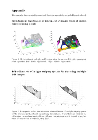
Simultaneous registration of multiple 3-D images without known
corresponding points
50
100
150
200
250
300
−50
0
50
100
150
200
250
300
50
100
150
X1
Y1
Z1
50
100
150
200
250
300
−50
0
50
100
150
200
250
300
80
100
120
140
160
X1
Y1
Z1
Figure 1: Registration of multiple profile maps using the proposed iterative parametric
point algorithm. Left: Initial registration. Right: Refined registration.
Self-calibration of a light striping system by matching multiple
3-D images
Figure 2: Four synthetic data sets before and after calibration of the light striping system
by the proposed method based on matching the surfaces. When there are errors in the
calibration, the surfaces acquired from different viewpoints do not fit to each other, but
when the calibration is corrected, they do fit.
1

2. Statistical analysis of two registration and modeling strategies
Figure 3: Precision of the modeled profile maps in a simultaneous registration strategy
with the model computed afterwards, as given by the statistical analysis performed. The
color ranges from blue through green and yellow to red as the precision decreases from
high to low. The statistical analysis takes into account all the error sources including
measurement, calibration, registration, and modeling uncertainties.
2

3. Detection of distortions in digital elevation models of glacial areas
after aligning the models accurately
x / m
y/10
6
m
28000 29500 31000 32500 34000 35500 37000 38500
5.192
5.1905
5.189
5.1875
5.186
5.1845
5.183
5.1815
−4
−3
−2
−1
0
1
2
3
4
m
hollow in IKONOS DEM
hollow in IKONOS DEM
edge in aerial photography DEM
aerial photography DEM distorted
Figure 4: Distortions detected in the aerial photography DEM and Ikonos DEM of Hin-
tereisferner glacier. The color shows the difference in elevation between the DEMs. The
detection of distortions is based on analyzing difference images between three or more
DEMs produced from data acquired on the same day.
Visualization of airborne laser scanner data on a terrestrial
panoramic image of a glacial area
Figure 5: Triangulated laser scanner data projected onto one of the terrestrial panoramic
images after registering the laser scanner data with a terrestrial photography DEM.
3

4. Derivation of estimates for the accuracy of change in elevation
and volume of a glacier
x / m
y/106
m
632000 633000 634000 635000 636000 637000 638000
5.191
5.19
5.189
5.188
5.187
5.186
−8
−6
−4
−2
0
2
4
6
8
m
ice−free area for precision estimation
ice−free area for precision estimation
Hintereisferner study area for change detection
0 100 200 300 400 500 600 700 800
−3
−2.5
−2
−1.5
−1
−0.5
0
0.5
1
1.5
2
x 10
7
time in days
changeinvolume/m3
Figure 6: Top: Changes in elevation at least occurred in Hintereisferner between August
19, 2002, and August 12, 2003, according to the error bounds derived, and differences
in elevation between the DEMs in ice-free test areas for precision estimation. Bottom:
Changes in volume (circles and solid line) with error bounds (dashed lines) in Hintereis-
ferner during a period of two years as estimated by the proposed method from a sequence
of ten laser scanner DEMs.
4

5. Correspondence matching between trunks estimated from a pair
of terrestrial images and from airborne laser scanner data
50 100 150 200
50
100
150
200
Figure 7: Left: Trunks extracted from the terrestrial image are shown as red lines and
trunks extracted from the laser scanner data and projected onto the image as green lines.
Right: The positions of the corresponding trunks found by the proposed method and the
viewing areas of the cameras visualized on a digital surface model of 0.5m × 0.5m ground
resolution.
3-D reconstruction from a stereo image sequence
Figure 8: Left: One image of the left camera. Right: Surface model of the trunk re-
constructed by the proposed method from a stereo image sequence captured onboard a
harvester approaching the tree.
5

6. 3-D deformation estimation from a single image or multiple im-
ages with weak imaging geometry
−10
−5
0
5
10
−10
−5
0
5
10
−2
−1.5
−1
−0.5
0
0.5
1
X / mY / m
Z/m
−5
0
5
−5
0
5
−1.5
−1
−0.5
0
0.5
X / mY / m
Z/m
Figure 9: True deformed surface in blue and the estimated deformed surface in red, when
the imaging geometry is weak. The traditional method gives mainly noise (left figure)
while the proposed method estimates the deformation accurately (right figure).
6

7. Detection of cameras the orientations of which have changed
when the object deforms at the same time
Figure 10: A plate monitored with four cameras. Upper left: A discrepancy measure
exceeds an adaptive threshold for image 2, which shows that the orientation of camera
2 has changed. Upper right: In red, the surface after deformation and correction of the
exterior orientation of camera 2 using the proposed method based on a shape function;
In dark blue, the deformed surface reconstructed using the traditional method; In cyan,
the surface before deformation given by iWitness software.
7

8. Tracking of facial deformations in multi-image sequences with
elimination of rigid motion of the head
Frame 35 Frame 50 Frame 70
Figure 11: Top: Tracked image points in one camera of a multi-image sequence. Bottom:
Large changes in the image coordinates without (left image) and with (right image) elim-
ination of the effect of rigid motion. The facial deformation around the mouth is correctly
pointed out in the right image.
8

9. Estimation of lower bounds for deviations of as-built structures
from an as-designed Building Information Model given a single
spherical panoramic image of the scene
Figure 12: From top to bottom: edge curves extracted from the spherical panoramic image
and initial orientation of the image with respect to a BIM; refined orientation; BIM model
adjusted to fit with the edge features of the image; adjusted BIM in 3-D space with color
illustrating differences against the as-designed BIM.
9

10. Shape function-based 3-D deformation estimation with moving
cameras attached to the deforming body
Figure 13: Deformation estimation of the frame of a crane by the proposed method, when
the cameras need to be attached to the self deforming body, the structure sways during
loading, and the imaging geometry is not optimal due to physical limitations.
10

11. Dense image matching and 3-D reconstruction from a pair of
scanning electron microscope images of a single atmospheric dust
particle
Figure 14: Top: SEM image of an aggregate particle. Bottom: Dense TIN model of over
million points reconstructed by the proposed method from a pair of SEM images.
11