The effect of VaR-based risk management on asset prices and the volatility smile

1. 348
The effect of VaR-based risk management on asset prices
and the volatility smile1
Arjan Berkelaar, World Bank,
2
Phornchanok Cumperayot, Erasmus University, Rotterdam,
and Roy Kouwenberg, Aegon Asset Management, The Hague
Abstract
Value-at-risk (VaR) has become the standard criterion for assessing risk in the financial industry. Given
the widespread usage of VaR, it becomes increasingly important to study the effects of VaR-based risk
management on the prices of stocks and options. We solve a continuous-time asset pricing model,
based on Lucas (1978) and Basak and Shapiro (2001), to investigate these effects. We find that the
presence of risk managers tends to reduce market volatility, as intended. However, in some cases VaR
risk management undesirably raises the probability of extreme losses. Finally, we demonstrate that
option prices in an economy with VaR risk managers display a volatility smile.
1. Introduction
Many financial institutions and non-financial firms nowadays publicly report value-at-risk (VaR), a risk
measure for potential losses. Internal uses of VaR and other sophisticated risk measures are on the
rise in many financial institutions, where, for example, a bank’s risk committee may set VaR limits, both
amounts and probabilities, for trading operations and fund management. At the industrial level,
supervisors use VaR as a standard summary of market risk exposure.
3
An advantage of the VaR
measure, following from extreme value theory, is that it can be computed without full knowledge of the
return distribution. Semi-parametric or fully non-parametric estimation methods are available for
downside risk estimation. Furthermore, at a sufficiently low confidence level the VaR measure explicitly
focuses risk managers’ and regulators’ attention on infrequent but potentially catastrophic extreme
losses.
Given the widespread use of VaR-based risk management, it becomes increasingly important to study
the effects on the stock market and the option market of these constraints. For example, institutions
with a VaR constraint might be willing to buy out-of-the-money put options on the market portfolio in
order to limit their downside risk. If multiple institutions follow the same risk management strategy, then
this will clearly lift the equilibrium prices of these options. Also the shape of the stock return distribution
in equilibrium will be affected by the collective risk management efforts. As a result, it might even be
the case that the distribution of stock returns will become more heavy-tailed. This would imply that the
attempt to handle market risk, and thus to reduce default risk, has adversely raised the probability of
such events.
Recently, Basak and Shapiro (2001) have derived the optimal investment policies for investors who
maximise utility, subject to a VaR constraint, and found some surprising features of VaR usage. They
show, in a partial equilibrium framework, that a VaR risk manager often has a higher loss in extremely
1
This article was first published in European Financial Management, vol 8, issue 2, June 2002, pp 139-64. The copyright
holder is Blackwell Publishers Ltd.
2
Corresponding author: World Bank, Investment Management Department (MC7-300), 1818 H Street NW, Washington DC
20433, USA, tel: +1 202 473 7941, fax: +1 202 477 9015, e-mail: aberkelaar@worldbank.org. This paper reflects the
personal views of the authors and not those of the World Bank. We would like to thank Suleyman Basak and Alex Shapiro for
their helpful comments.
3
The Bank for International Settlements (BIS) mandates internationally active financial institutions in the G10 countries to
report VaR estimates and to maintain regulatory capital to cover market risk.

2. 349
bad states than a non-risk manager. The risk manager reduces his losses in states that occur with
(100 – α)% probability, but seems to ignore the α% of states that are not included in the computation of
VaR. Starting from this equilibrium framework based on the Lucas pure exchange economy, in this
paper we aim to further investigate Basak and Shapiro’s (2001) very interesting and relevant question
regarding the usefulness of VaR-based risk management.
In our economic setup, agents maximise the expected utility of intermediate consumption up to a finite
planning horizon T and the expected utility of terminal wealth at the horizon. A portion of the investors
in the economy are subject to a VaR risk management constraint, which restricts the probability of
losses at the planning horizon T. As a result of our setup, asset prices do not drop to zero at the
planning horizon and, moreover, we can ignore the unrealistic jump in asset prices that occurs just
after the horizon of the VaR constraint, as in Basak and Shapiro (2001). We find that the VaR agents’
investment strategies, depending on the state of nature, directly determine market volatility, the
equilibrium stock price and the implied volatilities of options. In general VaR-based risk management
tends to reduce the volatility of the stock returns in equilibrium and hence the regulation has the
desired effect. In most cases the stock return distribution has a relatively thin left tail and positive
skewness, which reduces the probability of severe losses relative to a benchmark economy without risk
managers.
However, we also find that in some cases VaR-based risk management adversely amplifies default risk
through a relatively heavier left tail of the return distribution. In very bad states the VaR risk managers
switch to a gambling strategy that pushes up market risk. The adverse effects of this gambling strategy
are typically strong when the investors consume a large share of their wealth, or when the VaR
constraint has a relatively high maximum loss probability α. Additionally, we study option prices in the
VaR economy. We find that the presence of VaR risk managers tends to reduce European option
prices, and hence the implied volatilities of these options. Moreover, we find that the implied volatilities
display a smile, as often observed in practice, unlike the benchmark economy, where implied volatility
is constant.
We conclude that VaR regulation performs well most of the time, as it reduces the volatility of the stock
returns and it limits the probability of losses. However, in some special cases, the VaR constraint can
also adversely increase the likelihood of extremely negative returns. This negative side effect typically
occurs if the investors in the economy have a strong preference for consumption instead of terminal
wealth, or when the VaR constraint is rather loose (ie with high α). Note that the negative
consequences of VaR-based risk management are mainly due to the “all or nothing” gambling attitude
of the optimal investment strategy in case of losses, which might seem rather unnatural. In this paper
we argue that the gambling strategy of a VaR risk manager might not be that unnatural for many
investors, as it is closely related to the optimal strategy of loss-averse agents with the utility function of
prospect theory.
Prospect theory is a framework for decision-making under uncertainty developed by the psychologists
Kahneman and Tversky (1979), based on behaviour observed in experiments. The utility function of
prospect theory is defined over gains and losses, relative to a reference point. The function is much
steeper over losses than over gains and also has a kink in the reference point. Loss-averse agents
dislike losses, even if they are very small, and therefore their optimal investment strategy tries to keep
wealth above the reference point.
4
Once a loss-averse investor’s wealth drops below the reference
point, he tries to make up his previous losses by following a risky investment strategy. Hence, similar to
a VaR agent, a loss-averse agent tries to limit losses most of the time, but starts taking risky bets once
his wealth drops below the reference point. The optimal investment strategy under a VaR constraint
might therefore seem rather natural for loss-averse investors. Or, conversely, one could argue that a
VaR constraint imposes a minimum level of “loss aversion” on all investors affected by the regulation.
This paper is organised as follows: in Section 2, we define our dynamic economy and the
market-clearing conditions required in order to solve for the equilibrium prices. Individual optimal
investment decisions are also discussed. The general equilibrium solutions and analysis are presented
in Section 3. We focus on the total return distribution of stocks and the prices of European options in
the presence of VaR risk managers. Section 4 investigates the similarity between risk management
4
This behaviour is induced by the kink in the utility function, ie first-order risk aversion; see Berkelaar and Kouwenberg
(2001a).

3. 350
policies based on VaR and the optimal investment strategy of loss-averse investors. Section 4 finally
summarises the paper and presents our conclusions.
2. Economic setting
2.1 A dynamic economy
In this section, the pure exchange economy of Lucas (1978) is formulated in a continuous-time
stochastic framework. Suppose in a finite horizon, [0,T], economy, there are heterogeneous economic
agents with constant relative risk aversion (CRRA). The agents are assumed to trade one riskless bond
and one risky stock continuously in a market without transaction costs.
5
There is one consumption
good, which serves as the numeraire for other quantities, ie prices and dividends are measured in units
of this good. The bond is in zero net supply, while the stock is in constant net supply of 1 and pays out
dividends at the rate
t
d , for [ ]
T
t ,
0
Î . The dividend rate is presumed to follow a Geometric Brownian
motion:
6
t
dB
t
dt
t
t
d d
s
+
d
m
=
d @
@ (1)
with 0
m@ and 0
s@ constant.
The equilibrium processes of the riskless money market account S0(t) and the stock price S1(t) are the
following diffusions, as will be shown in Section 3.1:
dt
t
S
t
r
t
dS 0
0 = , (2)
t
dB
t
S
t
dt
t
S
t
t
t
dS 1
1
1 s
+
m
=
d
+ ,
where the interest rate r(t), the drift rate µ(t) and the volatility σ(t) are adapted processes and possibly
path-dependent.
As we assume a dynamically complete market, these price processes ensure the existence of a unique
state price density (or pricing kernel)
t
x , following the process
t
dB
t
dt
t
r
t
t
d
k
-
-
=
x
x
, 1
)
0
( =
x , (3)
where
t
t
r
t
t s
-
m
=
k / denotes the process for the market price of risk (Sharpe ratio).
Following from the law of one price, the pricing kernel
t
x relates future dividend payments
s
@ ,
]
T
t
s ,
Î to today’s stock price S1(t):
ú
û
ù
ê
ë
é d
x
x
= ò
T
t
t ds
s
s
E
t
t
S
1
1 . (4)
Intuitively the stock price is the price you pay to achieve a certain dividend in each state at each time t.
Equation (4) is simply an over-time summation of the Arrow-Debreu security prices, discounting the
future dividend payouts to today’s value. The state price density process will therefore play an
important role in deriving the equilibrium prices.
5
Basak and Shapiro (2001) assume N risky assets. However, our results are robust to the number of assets.
6
All mentioned processes are assumed to be well defined and satisfy the appropriate regularity conditions. For technical
details, see Karatzas and Shreve (1998).

4. 351
2.2 Preferences, endowments and risk management
Suppose there are two groups of agents in the economy: non-risk-managing and risk-managing
agents. Agents belonging to the former group freely optimise their investment strategy, ie without risk
management constraints, whereas the latter group is obligated to take a VaR restriction as a side
constraint when structuring portfolios.
7
We assume that a proportion l of the agents is not regulated,
while the remaining proportion (1 – l ) is. Each agent is endowed at time zero with initial wealth Wi(0).
We use subscript i = 1 for the unregulated agents and i = 2 for the risk managers. For both groups of
agents we define a non-negative consumption process ci(t) and a process for the amount invested in
stock πi(t). The wealth Wi(t) of the agents then follows the process below:
t
dB
t
t
dt
t
c
dt
t
t
r
t
dt
t
W
t
r
t
dW i
i
i
i
i p
s
+
-
p
-
m
+
= , (5)
for i = 1, 2; [ ]
T
t ,
0
Î
.
As in the case of asset prices, today’s wealth can be related to future consumption and terminal wealth
through the state price density process
t
x :
ú
û
ù
ê
ë
é x
+
x
x
= ò
T
t i
i
t
i T
W
T
ds
s
c
s
E
t
t
W
1
. (6)
The agents maximise their utility from intertemporal consumption in [0,T] and terminal wealth at the
planning horizon T, which are represented by Ui(ci(t)) and Hi(Wi(T)) respectively. The parameter 0
1
r
determines the relative importance of utility from terminal wealth compared to utility from consumption.
The planning problem for an unregulated agent then is:
1
1,
max F
c ú
û
ù
ê
ë
é r
+
ò
T
T
W
H
ds
s
c
U
E 0 1
1
1
1
1 ))
(
(
))
(
( .
s.t.
t
dB
t
t
dt
t
c
dt
t
t
r
t
dt
t
W
t
r
t
dW 1
1
1
1
1 p
s
+
-
p
-
m
+
= , (7)
,
0
1 ³
t
W for [ ]
T
t ,
0
Î
.
Additionally, in order to limit the likelihood of large losses, the risk managers have to take a VaR
constraint into account. Based on the practical implementation of VaR and its interpretation by Basak
and Shapiro (2001), at the horizon T the maximum likely loss with probability (1 – α)% over a given
period, namely VaR(α), is mandated to be equal to or below a prespecified level. More precisely, the
agents are allowed to consume continuously but make sure that, only with probability α% or less, their
wealth W2(T) falls below the critical floor level W. Therefore, the second group of agents faces the
following optimisation problem with the additional VaR constraint:
2
2 ,
max F
c
ú
û
ù
ê
ë
é r
+
ò T
W
H
ds
s
c
U
E
T
2
2
2
0 2
2
s.t.
t
dB
t
t
dt
t
c
dt
t
t
r
t
dt
t
W
t
r
t
dW 2
2
2
2
2 p
s
+
-
p
-
m
+
= , (8)
0
2 ³
t
W , for [ ]
T
t ,
0
Î
,
[ ] a
-
³
³ 1
2 W
T
W
P .
We assume that all agents have constant relative risk aversion over intertemporal consumption
t
c
V
t
c
U i
CRRA
i
i = and over terminal wealth
T
W
V
T
W
H i
CRRA
i
i = for i = 1, 2, where VCRRA (·) is a
power utility function:
g
-
g
-
= 1
1
1
x
x
VCRRA , for 0
g ; 0
x . (9)
7
It should be noted that the superfluous risk management critique (see Modigliani and Miller (1958), Stiglitz (1969a,b and
1974), DeMarzo (1988), Grossman and Vila (1989) and Leland (1998)), does not hold at the individual level. The critique
states that risk management is irrelevant for institutions and firms since individuals can undo any financial restructuring by
trading in the market. This paper considers individual agents, and hence this line of reasoning is invalid here.

5. 352
Note that the power utility function (9) is increasing and strictly concave and hence agents are
assumed to be risk-averse. By assuming a common power utility function for intertemporal
consumption and terminal wealth, we can isolate the effect of VaR-based risk management on asset
prices. Our main purpose is to study the influence of risk management on the equilibrium price of the
risky asset and on option prices.
In this paper, the VaR horizon coincides with the investment horizon, which is different from Basak and
Shapiro’s (2001) work. In their work, agents are concerned with the optimal consumption path over
their lifetime, while obligated to a one-time-only risk evaluation. The VaR condition is supposed to be
satisfied at some intermediate time, before the end of the agent’s life. As a consequence of this setup,
a severe jump in the price level occurs when the VaR condition is lifted. In addition, since agents
consume everything at the planning horizon T and wealth drops to zero at that time, the corresponding
asset prices go to zero.
In this paper, the horizon is just a subperiod of the lifetime in Basak and Shapiro (2001). Thus, agents
can evaluate their VaR performance at the end of each period, eg a 10-day or an annual report, along
the way maximising the utility from their intertemporal consumption as well as their terminal wealth. In
our perspective, this adjustment makes the model more realistic. At the horizon agents may end up
with claims on the assets and prices do not necessarily drop to zero. Moreover, within our setup we
can ignore the jump in asset prices that occurs directly after the VaR horizon in Basak and Shapiro
(2001). Note that this jump in asset prices occurs because all regulated investors drop the VaR
constraint collectively, at a prespecified point in time. We think that such a coordinated abandonment of
risk management policies is rather hypothetical and therefore we do not analyse the consequences of
a jump in asset prices in this paper.
2.3 Equilibrium conditions and optimal decisions
In order to investigate the equilibrium asset prices in an economy with VaR risk managers, in this
section we discuss the conditions that should be satisfied in any general equilibrium. In equilibrium,
each agent optimises his individual consumption-investment problem. Moreover, as the consumption
good cannot be stored, it follows that aggregate consumption in the economy has to equal aggregate
dividends at each time [ ]
T
t ,
0
Î . Additionally, from Walras law it follows that all markets have to clear,
eg the good and the riskless securities markets, given that the stock market is in equilibrium at each
time [ ]
T
t ,
0
Î . Combined, this gives the following set of equilibrium conditions:
t
t
c
t
c d
=
l
-
+
l *
*
2
1 1 , (10)
t
S
t
t 1
2
1 1 =
p
l
-
+
lp *
*
,
t
S
t
W
t
W 1
2
1 1 =
l
-
+
l *
*
,
where
t
c*
1 and
t
*
F1 are the optimal consumption and investment decisions for each type of agent
i = 1, 2 and )
(
*
t
Wi is the corresponding optimal wealth process.
Typically the optimal policies for agents with power utility can be derived with dynamic programming,
as in Merton (1969), as well as with the martingale methodology of Cox and Huang (1989), Karatzas et
al (1987) and Pliska (1986). However, for the risk managers, the binding VaR restriction induces non-
concavity into the optimisation problem (through the wealth function). Following Basak and Shapiro
(2001), we derive the optimal policies for the regulated agents with power utility by applying the
martingale methodology. The dynamic optimisation problem melts down to the following problem:
i
i
c F
,
max
ú
û
ù
ê
ë
é r
+
ò T
W
H
ds
s
c
U
E i
i
i
T
i
i
0
s.t.
0
0
0 i
T
i
i W
T
W
T
ds
s
c
s
E x
£
ú
û
ù
ê
ë
é x
+
x
ò , (11)
0
³
T
Wi ,
for i = 1, 2, with an additional constraint for the risk managers:
[ ] a
-
³
³ 1
2 W
T
W
P . (12)

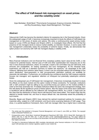
6. 353
In the next proposition we characterise the optimal consumption paths and terminal wealth profiles for
both groups of agents:
Proposition 1
For any state price density following the process (3), the optimal intertemporal consumption policies
t
c*
1 and terminal wealth profiles
T
Wi
*
of both groups of agents i = 1, 2 are
g
-
*
x
=
x
=
1
1
1
1
1 t
y
t
y
I
t
c , (13)
g
-
*
x
=
x
=
1
2
2
2
2 t
y
t
y
I
t
c ,
g
-
*
r
x
=
1
1
1
1 T
y
T
W ,
2
2
2 H
N T
y
I for x
x T
=
*
T
W2 W for x
£
x
£
x T
2
2
2 H
N T
y
I for
T
x
£
x
where Ii(z) denotes the inverse of the marginal utility function
x
U
z i
'
= , 2
'
2
2 y
W
U
r
=
x , x is such
that
[ ] a
=
x
x T
P and 0
³
i
y is a Lagrange multiplier that satisfies
0
0
0 i
T
i
i W
T
W
T
ds
s
c
s
E x
=
ú
û
ù
ê
ë
é x
+
x
ò
*
*
, for i = 1, 2. (14)
In order to facilitate the derivation of equilibrium prices in the following sections, we additionally use the
following proposition proved by Karatzas et al (1990) and Basak (1995). It provides a different
representation of the equilibrium conditions by applying the martingale methodology.
Proposition 2
If there exists a state price density process ξ(t) satisfying
t
y
I
t
y
I
t x
l
-
+
x
l
=
d 2
2
1
1 1 , (15)
where y1 and y2 are Lagrange multipliers defined in (14), then the equilibrium conditions (10) are
satisfied by the corresponding optimal consumption and investment policies.
Before we actually derive the equilibrium prices, we will first discuss the optimal investment strategies
in partial equilibrium of the unrestricted agents (benchmark agents), the regulated agents (the VaR risk
managers) and the portfolio insurers. Portfolio insurers are VaR risk managers that do not tolerate any
losses below W, ie they represent the extreme case α = 0.
8
It is noteworthy that portfolio insurers fully
insure against all states of nature at the minimal wealth level W, whereas VaR risk managers with α 0
only partially insure. VaR risk managers with α 0 do not necessarily insure in expensive states that
occur with very low probability.
In Figure 1, we display the optimal terminal wealth profiles for the three types of agents. All agents
have initial endowment of W(0) = 1 and power utility over consumption and over terminal wealth with
risk aversion parameter g = 1, which is in limit equivalent to log utility. We set the trade-off between
consumption and terminal wealth at ρ1 = ρ2 = 10, to avoid excessive consumption. The maximum loss
probability α of the risk managers and the portfolio insurers is equal to 1% and 0 respectively. The
critical wealth W at time T = 1 is 0.95. The interest rate and the Sharpe ratio are given by 5% and 0.4.
Endogenous thresholds, x and x , are then calculated.
8
See Basak (1995), Basak and Shapiro (1999), Grossman and Vila (1989) and Grossman and Zhou (1996).
ï
ï
î
ï
ï
í
ì

7. 354
To be more specific, throughout the paper, states of the world are roughly classified into three ranges.
First, good states are the states in which the VaR constraint is not binding since the optimal (terminal)
wealth, as a consequence of individual optimisation, is likely to be above or equal to the minimal wealth
threshold. Second, intermediate states ]
x
x, are the states in which the unrestricted individual’s wealth
is likely to end up below the threshold. Thus, VaR risk management becomes binding in these states.
Last, extremely bad states are the small area of worst cases with a total probability mass of α. In these
states the VaR managers will no longer try to keep wealth above W. Note that sizes of these ranges
depend on the minimal wealth threshold W and the probability of loss α for the VaR managers.
Figure 1 shows that the optimal terminal wealth function of the benchmark agents is decreasing
smoothly from good states of the world (low
T
x ) to bad states (high
T
x ), whereas the partial
insurers and full insurers behave differently. In the good states region (low
T
x ), they all have
smoothly decreasing curves. However, for the portfolio insurers to guarantee terminal wealth in
intermediate and extreme states, from x onwards, they have to pay based on the pricing kernel, ie the
worse the state implies the higher the price to obtain a fixed amount of wealth in that particular state.
Therefore, the portfolio insurers consume relatively less in good states in order to pay for the insurance
in bad states.
Unlike the portfolio insurers, the VaR-based risk managers are not obligated to insure in the most
expensive states (high
T
x ). In very bad states, from x onwards, terminal wealth dramatically drops
and remains lower than the benchmark level. In terms of probability, the VaR managers have high
probability of achieving the critical wealth threshold that they insure in intermediate states. However,
lower payoff in bad states leads to a heavier tail in the lower quantiles of the wealth distribution,
compared to other types of investors. Note that the area on the right of x contains only α% of
probability mass. Hence, the area where the VaR risk manager tolerates losses is less probable than it
might seem in the figure.
Next we analyse the dynamic (state-varying) optimal investment policies of the VaR managers relative
to the benchmark agents and the portfolio insurers. In order to do so, we assume for now Geometric
Brownian motions for the dividend rate and the stock price with constant interest rate r = 5% and
constant market price of risk κ = 0.4. Later on we will see that in the general equilibrium framework the
interest rate and the market price of risk are indeed constant. As in the previous example, initial wealth
is W(0) = 1 and T = 1, while the current time is t = 0.75.
In Figure 2, the optimal wealth of three kinds of investors is shown at an intermediate point in time
(t = 0.75). The figure demonstrates the common feature of a steeply decreasing wealth function, with a
slower descent as the states are worsening. As in Figure 1, the benchmark agent’s wealth is a
decreasing convex function, while the portfolio insurers always keep their wealth above the level
exp(–r(T – t))W. The time-t wealth profile of the VaR risk manager with α = 1% lies in between these
two extremes. It looks like a smoothed version of the terminal wealth profile at the horizon T, without
the abrupt jump at x .
Figure 3 displays the optimal portfolio weight of stocks relative to the benchmark. It reveals how
VaR-based investors change their investment strategy to insure their terminal wealth. In good states
the VaR risk-managing agents follow the benchmark behaviour. In the middle range, when the state
price is relatively low they replicate the portfolio insurers’ strategy, which is to invest in riskless assets.
In bad states the VaR agents greatly increase their exposure to the risky asset, as they try to maximise
the probability of their wealth staying above the critical threshold W. However, to avoid bankruptcy, the
risk managers eventually reduce their risk exposure again.
9
Concluding: the VaR restriction reduces the exposure to risky assets in good states relative to the
benchmark, while in extremely bad states it stimulates risky-asset holding in a desperate attempt to
make up for low wealth (gambling). Thus, outside the area where the VaR constraint is binding,
logically the VaR agents’ wealth is always lower than in the benchmark case. In the following section,
9
Please note that states with a pricing kernel higher than three in Figure 3 have almost no probability of occurring and are
only shown for illustrative purposes.

8. 355
we will investigate the impact of this investment strategy on market risk, the equilibrium asset prices
and the total return distribution. The usefulness of VaR regulation, implicitly or explicitly, will be
discussed in Section 5.
3. General equilibrium with VaR risk managers
3.1 Closed-form solutions
In this section, we expand the individual optimisation problem of the previous section to a Lucas
general equilibrium model, based on the market clearing conditions (10). In the economy, there is a
fraction l of agents, who are unrestricted, and the remaining fraction 1 – l , who apply VaR-based risk
management. Our economy is formulated such that, in some subperiod, agents maximise their utility
from intermediate consumption, [ ]
T
t ,
0
Î , and from terminal wealth at the horizon T. The VaR
restriction is imposed on the risk managers at time T, coinciding with their planning horizon.
As a first step in solving the equilibrium model, it is convenient to derive the equilibrium state price
density as a function of aggregate dividends by inverting equation (15). Given the stochastic process
for the state price density in (3), as a second step we can infer the equilibrium interest rate and market
price of risk. The following proposition summarises these general results:
Proposition 3
In any economy with 1
0 £
l
£ equilibrium exists and the state price density is given by
g
-
d
=
x t
y
y
v
t 2
1, , (16)
where
1
1
2
1
1
2
1 1
,
-
g
-
g
-
l
-
+
l
= y
y
y
y
v . (17)
The equilibrium interest rate and market price of risk processes are constant:
2
1
2
1 @
@ s
g
+
-
m
g
=
t
r , (18)
@
gs
=
t
k .
An important conclusion from proposition (3) is that the interest rate r and the market price of risk k are
constant in equilibrium. Furthermore, the fraction of risk managers in the economy does not affect the
interest rate and the market price of risk. Hence, in our setup the presence of risk managers will only
have an impact on the price level of the stock, on its drift rate µ and volatility σ. Note, however, that the
mean and volatility always have to move in lockstep due to the constant market price of risk. In
addition, based on the assumption of a Geometric Brownian for the dividend process, equation (16)
implies a log-normal state price density.
The constant interest rate and market price of risk arise due to the assumption that both groups of
agents share an identical power utility function over intertemporal consumption. Although this economic
setup leads to some inflexibility, a major advantage is that we can derive closed-form solutions for the
equilibrium prices and hence fully analyse the economic problem at hand. Basak (1995) and Basak
and Shapiro (2001) also impose equivalent assumptions in order to study equilibrium with portfolio
insurers and value-at-risk regulation respectively. Without an identical utility function over consumption
for both groups of agents, we would have to resort to numerical techniques as in Grossman and Zhou
(1996).
10
10
The same holds if we leave out consumption and only assume utility over terminal wealth.

9. 356
Given the state price density of proposition (3), we can derive the equilibrium stock price from the
equilibrium conditions (10). Once a closed-form expression has been obtained, the drift rate µ and
volatility σ of the stock price process follow straightforwardly from Ito’s lemma. Below we first present
the equilibrium price in a benchmark economy with unrestricted investors only ( l = 1), before we
consider our general results in the presence of risk managers:
Proposition 4
The equilibrium price of the risky asset in an economy with unregulated agents only ( l = 1) is
t
T
e
t
a
t
t
S -
h
g
r
+
d
= 1
1
1 , (19)
with
1
1
-
h
= -
h t
T
e
t
a , 2
1
2
1
1 d
d s
g
-
g
-
m
g
-
=
h . (20)
The stock price follows a Geometric Brownian motion with constant drift rate and volatility given by
2
1
2
1 @
@ s
g
-
+
m
g
=
m t , @
s
=
s t . (21)
In the case of unregulated agents with power utility, the interest rate is constant and the stock price
follows a Geometric Brownian motion, resembling the familiar Black-Scholes assumptions for option
pricing. As a result, it has a log-normal (Gaussian-class) distribution. If we additionally introduce
VaR-based risk managers ( l 1), then the equilibrium stock price process changes quite drastically:
Proposition 5
The equilibrium price of the risky asset in an economy with both unregulated agents and VaR risk
managers is
t
e
y
y
v
y
t
t
a
t
S t
T
d
r
l
+
d
= -
h
g
-
2
1
1
1
1
1 , (22)
x
d
-
+
x
d
-
-
d
r
l
-
+ G
g
-
,
,
,
,
1
,
1 2
1
1
2
2 t
t
d
N
t
t
d
N
t
e
y
y
v
y t
x
d
-
-
x
d
-
l
-
+ -
-
,
,
,
,
1 t
t
f
N
t
t
f
N
e
W t
T
r
with
t
T
t
T
r
y
y
v
t
x
x
t
f
-
k
-
k
-
+
+
d
g
+
=
d
2
2
1
2
1,
log
log
log
,
, , (23)
t
T
x
t
f
x
t
d -
k
g
+
d
=
d
1
,
,
,
, (24)
t
T
t
T
r
t -
k
÷
÷
ø
ö
ç
ç
è
æ
g
g
-
+
-
÷
ø
ö
ç
è
æ
k
+
g
g
-
=
G 2
2
2 1
2
1
2
1
1
(25)
and N(·) is the standard-normal cumulative distribution function.
In an economy with VaR-regulated investors, the drift rate µt and the volatility σt of the stock price
process are no longer constant, which can be easily verified by applying Ito’s lemma to the stock price
formula (22). Figures 4 and 5 show that at a point in time the expected drift rate and the volatility can
be either high or low relative to the benchmark case, depending on the state of the world. In the next
section we will analyse these drift rates and the volatility processes. Moreover, the impact of
VaR-based risk management on the equilibrium stock price, its total return distribution and the
equilibrium option prices will be examined respectively.

10. 357
3.2 Drift rate, volatility and prices in equilibrium
For the numerical examples, we set the parameters of the dividend process as 056
.
0
=
m@ and
115
.
0
=
s@ , based on monthly SP 500 index data from 1980 up to 1999. All agents have initial wealth
W(0) = 1 and maximise a power utility over intertemporal consumption and terminal wealth with risk
aversion g = 1. We set the trade-off between consumption and terminal wealth at ρ1 = ρ2 = 10. The
maximum loss probability α is 100%, 1% and 0 respectively for the unregulated agents, the risk
managers and the portfolio insurers. The critical wealth W threshold at the planning horizon T = 1
is 0.95, while the current time is t = 0.75. The insurer economy and the risk manager economy both
contain 50% of the benchmark agents and 50% of their own population (ie l = 1/2).
In order to take a closer look at the stock price process, first we present the expected drift rate and the
volatility of the stock returns as functions of the pricing kernel. In Figures 4 and 5, one can see that in
all three types of economies the market volatility and the drift rate move in lockstep as a consequence
of the constant market price of risk. In the benchmark economy, the mean and the volatility of the stock
price are constant in every state at all times, corresponding to the Black-Scholes assumptions for
option pricing. In the portfolio insurance economy, the expected returns and the volatility are lower in
most states, compared to the benchmark. Intuitively, the portfolio insurers want to hold less equity. In
order to clear the market, the attractiveness of stocks has to be increased and, hence, the equilibrium
volatility is reduced. The portfolio insurance strategy therefore reduces volatility and stabilises the
economy.
For exactly the same reasons, the volatility is reduced in intermediate states in the partially insured
VaR economy. However, in bad states the VaR agents abandon the portfolio insurance strategy and
instead they start to increase their demand for risky assets, as can been seen in Figure 3.
11
The
overwhelming demand caused by this gambling policy leads to a relatively high volatility and drift rate,
in order to clear the market. Eventually, in very bad states, the portfolio weight of the VaR agents
returns to normal levels in order to avoid bankruptcy. As a result, the equilibrium volatility and drift rate
are then pulled back to the benchmark level.
We will now analyse the consequences of the presence of VaR risk managers on the equilibrium stock
price. Figure 6 displays the equilibrium price of the risky asset in different states of nature, ranging from
good to bad, for the benchmark economy with l = 1 and the mixed economies with l = 1/2, at the
intermediate time t = 0.75. For all economies, the price of the risky asset is generally high in good
states of the world (low
t
x ) and low in bad states (high
t
x ). This follows from the inverse relation
between the state price density and aggregate dividends in proposition 3, namely a higher pricing
kernel level implies lower aggregate dividends and consequently a lower stock price.
We start by explaining the price function in the portfolio insurance economy (the dotted line). In good
states the price function in the economy with portfolio insurers has a similar shape as in the benchmark
case; however, it lies at a lower level. This follows from the fact that the constrained agents have less
wealth and therefore they demand less stocks: the equilibrium price has to be lower in order to clear
the market. In intermediate and bad states, the prices in the portfolio insurance economy are higher
than in the benchmark economy. In these states the equilibrium volatility in the portfolio insurance
economy is considerably lower than in the benchmark case. The low volatility increases the demand for
stocks and hence also increase the equilibrium price.
The price function in the economy with VaR risk managers is similar to the pattern in the portfolio
insurance economy in good and intermediate states. However, in bad states, the VaR risk managers
switch from the portfolio insurance strategy to a risky gambling strategy and this alters the shape of the
price function. Due to the increased demand for stocks in bad states, the volatility increases in order to
clear the market. While volatility increases and makes the stock less attractive, the price function drops
rather fast and ends up below the benchmark case. Finally, in extremely bad states, the VaR agents
reduce their risk exposure to avoid bankruptcy, volatility returns to regular levels and the shape of the
price function becomes similar to the benchmark case again.
11
Note that Figure 3 is not used for a quantitative analysis but for qualitative interpretation only, since the drift rate and volatility
do not coincide with the equilibrium case in Figures 4 and 5.

11. 358
3.3 The return distribution and option prices in equilibrium
Figures 7, 8 and 9 show the annualised total return distribution of the stock, including the estimated
divided yield. As the dividend payout rate changes stochastically through time, an exact calculation of
the total dividend payments would require extensive simulation. Instead we approximate the stochastic
dividend payout
ò @
t
dz
z
0
between time zero and t by
t
t 0
d
-
d . As the dividend process is the same
in each economy, we do not think that the error inherent in this approximation will have a serious
impact on our analysis or conclusions.
In the benchmark economy, the returns are log-normally distributed with slight positive skewness and
kurtosis close to three, as the stock price follows a Geometric Brownian motion. Figure 7 shows the
effect on the stock return distribution of a VaR constraint applied to 50% of the investors (ie l = 50%),
with critical wealth level W = 0.95 and maximum loss probability α = 0%, 1% and 5%. In an economy
with VaR risk managers or portfolio insurers, the volatility of the stock return distribution is clearly
lower. Moreover, the probability of negative returns up to –25% has also decreased substantially.
Hence, the VaR restriction seems to stabilise the economy. Note, however, that the probability of
negative returns in excess of –25% has increased in the case of a loose VaR constraint with α = 5%,
due to increased risk-taking at lower levels of wealth.
Figure 8 shows the return distribution in economies with a VaR constraint with α = 1%, at different
critical wealth levels W = 0.90, 0.95 and 0.99. The volatility of the stock returns tends to decrease as
the critical wealth level becomes higher and hence the VaR constraint becomes tighter. Note that in the
case of a very tight constraint, with W = 0.99, the left tail of the distribution becomes thicker and
extreme returns below –30% are more likely than in the unregulated economy. In general, though, the
economies with a VaR constraint are less volatile and the regulation has the intended effect.
Another important parameter affecting the economy is ρi, which determines the trade-off between the
utility of intertemporal consumption and the utility of terminal wealth. The previous computations were
made with ρ1 = ρ2 = 10, putting emphasis on terminal wealth. Figure 9 shows the return distribution in
an economy where intertemporal consumption is more important, with ρ1 = ρ2 = 1. In this case the left
tail of the distribution in the VaR economy becomes quite thick. The investors consume a large share
of their wealth and therefore have more difficulties meeting the VaR constraint in case of losses: this
leads to a more risky investment strategy and hence a heavy left tail.
So far, we have found that the presence of risk managers has a profound impact on the equilibrium
stock price and its return distribution. Now we will concentrate on the option market for European call
and put contracts. The prices of these options can be computed easily by discounting the payoffs at
maturity with the pricing kernel, as in no-arbitrage equation (4). The option payoffs are a function of the
equilibrium stock price, which we have derived in closed form. We only have to compute the
expectation in equation (4), which can be implemented straightforwardly as the pricing kernel follows a
Geometric Brownian motion. Once we have calculated the option prices for a wide range of strike
prices, we transform them into implied volatilities with the Black-Scholes formula, in order to facilitate
interpretation and comparisons.
Figure 10 shows the implied volatility in economies with a VaR constraint (α = 0%, 1% and 5%) and in
the benchmark economy. In the benchmark case we observe a constant implied volatility, following
from the Geometric Brownian motion of the stock price and the constant interest rate. In the economies
with a VaR constraint a remarkable option smile can be recognised, as often observed in practice. Note
that the implied volatility in economies with a VaR constraint is lower than in the benchmark case most
of the time. Moreover, as the VaR constraint becomes more strict (ie from α = 5% to α = 0%), the
implied volatility decreases. Similar volatility smiles can be observed if we change other parameters of
the VaR economy such as W and ρ2. Option prices are generally lower in VaR economies, as a result
of the reduced volatility of the stock return distribution.
4. VaR risk management and loss aversion
The equilibrium analysis in the previous section shows that, in general, VaR-based risk management
reduces the volatility of stock returns. However, in some cases the VaR constraint adversely increases
the probability of extreme losses. The negative consequences of VaR-based risk management are
mainly due to the “all or nothing” gambling attitude of the optimal investment strategy in case of losses,

12. 359
which might seem rather unnatural. In this section our aim is to demonstrate that the gambling strategy
of a VaR risk manager might not be that unnatural for many investors, as it is closely related to the
optimal strategy of loss-agents with the utility function of prospect theory.
Prospect theory was proposed by Kahneman and Tversky (1979) as a descriptive model for decision-
making under uncertainty, given the strong violations of the traditional utility paradigm observed in
practice. In experiments, Kahneman and Tversky (1979) found that people are concerned about
changes in wealth, rather than the level of wealth itself. Moreover, individuals treat gains and losses
relative to their reference point differently: the pain of a loss is felt much more strongly than the payoff
of an equivalent gain. Furthermore, in the domain of gains people are risk-averse, while they become
risk-seeking in the domain of losses.
Kahneman and Tversky (1979) quantified these empirical findings in prospect theory: individuals
maximise an S-shaped value function (26), which is convex for losses and concave for gains relative to
the reference point θ:
for q
£
x (26)
for q
x ,
where A 0 and B 0 to ensure that ULA(·) is an increasing function and 1
0 £
g
L , 1
0 £
g
G .
Moreover, A B holds in the case of loss aversion. The parameters of the loss-averse utility function
were estimated by Tversky and Kahneman (1992) as g L = g G = 0.88 and A/B = 2.25, based on
experiments. An illustration of the value function can be found in Figure 11. We denote agents who
maximise this value function with A B as “loss-averse”.
Berkelaar and Kouwenberg (2001a) derive the optimal wealth profile of a loss-averse investor, in a
similar dynamic economy as in Section 2 of this paper:
Proposition 6
For any state price density following the process (3), the optimal intertemporal consumption policy
t
cLA
*
and terminal wealth profiles
T
WLA
*
of a loss-averse agent are
1
1 -
g
*
x
=
x
= t
y
t
y
I
t
c LA
LA
LA , (27)
for LA
y
T x
x (28)
for LA
y
T x
³
x ,
where I(z) denotes the inverse of the marginal utility function over consumption z = U’(x), and N solves
0
=
x
f with
L
LA
G
LA
G
G
A
x
B
x
x
f G
G
G
g
g
-
g
-
g
q
r
+
q
-
g
r
÷
ø
ö
ç
è
æ
g
g
-
=
1
1
1
1
1
(29)
and 0
³
LA
y is a Lagrange multiplier, satisfying
0
0 LA
T
t LA
LA W
T
W
T
ds
s
c
s
E x
=
ú
û
ù
ê
ë
é x
+
x
ò
*
*
. (30)
Figure 12 shows the portfolio weights corresponding to this optimal wealth profile for a loss-averse
investor that puts more emphasis on terminal wealth than on consumption (ρLA = 100), assuming a
constant interest rate r = 5% and a constant Sharpe ratio κ = 0.4. Note that the investment strategy of
the loss-averse agent is qualitatively similar to the optimal policy of a VaR constrained agent. The
strategy is cautious in good states of the world with a low pricing kernel, and more risky in bad states of
ï
î
ï
í
ì
q
-
+
-
q
-
= C
C
,
,
G
L
LA
x
B
x
A
x
U
ï
î
ï
í
ì
÷
÷
ø
ö
ç
ç
è
æ
g
r
x
+
q
=
-
g
*
0
1
1 G
G
LA
LA
LA B
T
y
T
W

13. 360
the world with a high pricing kernel. Loss-averse agents dislike losses, even if they are very small, and
therefore their optimal investment strategy tries to keep wealth above the reference point in good
states of the world by investing more wealth in the riskless asset.
12
Once a loss-averse investor’s wealth drops below the reference point, he tries to make up his losses by
following a risky investment strategy. The risk-seeking behaviour stems from the convex shape of the
utility function of prospect theory below the reference point. Hence, similar to a VaR agent, a
loss-averse agent tries to limit losses most of the time, but starts taking risky bets once his wealth
drops below the reference point. The optimal investment strategy under a VaR constraint might
therefore seem rather natural for loss-averse investors. Or, conversely, one could argue that a VaR
constraint imposes a minimum level of “loss aversion” on all investors affected by the regulation.
Not surprisingly, loss-averse agents have a similar impact on asset prices in equilibrium as
VaR-constrained agents. We refer to Berkelaar and Kouwenberg (2001b) for a closed-form solution of
the asset price in a dynamic economy with loss-averse agents. Figure 13 compares the stock return
distribution in an economy with 50% loss-averse agents to an economy with 50% VaR-constrained
agents, while Figure 14 shows the volatility smile in the economies. Both figures demonstrate a clear
resemblance in prices. We conclude that asset prices in an economy with a VaR constraint correspond
qualitatively to prices in an economy with loss-averse investors who put emphasis on terminal wealth.
5. Conclusions
In order to investigate the effect of VaR-based risk management on asset prices in equilibrium, we
adopted the continuous-time equilibrium model of Basak and Shapiro (2001). The asset pricing model
is modified such that agents maximise their expected utility from intermediate consumption and
terminal wealth at the planning horizon. While dynamically optimising their consumption-investment
plan, the VaR restriction is imposed on the investors at the planning horizon. The VaR horizon thus
coincides with the investment horizon and can be interpreted as a subperiod of the investor’s lifetime
(eg an official reporting period of 10 days or one year). Within this setup we can ignore two unrealistic
price movements that occur in the model of Basak and Shapiro (2001); (1) a jump in prices just after
the VaR horizon, and (2) prices dropping to zero at the planning horizon.
We derived the closed-form equilibrium solutions for the asset prices in the model. Our main findings
are as follows: the presence of VaR risk managers generally reduces market volatility. However, in
very bad states the optimal investment strategy of VaR risk managers is to take a large exposure to
stocks, pushing up market risk and creating a hump in the equilibrium price function. In some special
cases this strategy can adversely increase the probability of extreme negative returns. This effect is
amplified in economies where investors consume a large share of their wealth, in economies where the
VaR constraint has a high maximum loss probability α and in economies with a high VaR threshold W.
We also derived the prices of European options in our economy and found that implied volatility is
typically lower in the presence of VaR risk managers. Moreover, VaR risk management creates an
implied volatility smile in our economy, as often observed in practice. As a final conclusion, we would
like to stress that VaR-based risk management has a stabilising effect on the economy as a whole for
most parameter settings in our model. However, it is important to note that the VaR restriction in some
cases might worsen catastrophic states that occur with a very small chance, due to the gambling
strategy of the VaR risk managers in bad states of the world.
The gambling strategy of VaR-based risk managers in bad states of the world is optimal within a
standard dynamic investment model, but might seem rather unnatural for investors in the real world. In
the last section of the paper we demonstrated that this gambling strategy in bad states is shared by
loss-averse investors, who maximise the utility function of prospect theory (Kahneman and
Tversky (1979)). As the optimal investment strategies of loss-averse agents and VaR risk managers
are quite similar, it might be relatively easy for the group of loss-averse investors to adopt VaR-based
risk management.
12
See footnote 4.

14. 361
Appendix
Proof of proposition 1
We refer to Cox and Huang (1989), Karatzas et al (1987) and Pliska (1986) for the optimal
consumption and investment policies for agents with power utility. Basak and Shapiro (2001) derive the
optimal policies for the portfolio choice problem with an additional VaR constraint.
Proof of proposition 2
This proof can be found in Karatzas et al (1990) and Basak (1995).
Proof of proposition 3
If we substitute the optimal consumption policies (13) into equilibrium relationship (15), then we find:
g
-
g
-
g
-
g
-
g
-
x
l
-
+
l
=
x
l
-
+
x
l
=
d
1
1
2
/
1
1
1
2
1
1 1
1 t
y
y
t
y
t
y
t , (31)
and hence the state price density in equilibrium is
g
-
g
-
g
g
-
g
-
d
=
d
l
-
+
l
=
x t
y
y
v
t
y
y
t 2
1
/
1
2
/
1
1 ,
1 . (32)
By applying Ito’s lemma, we can derive that ξ(t) follows the stochastic process below:
t
dN
t
dB
t
y
y
v
dt
t
y
y
v
g
-
d
g
-
d
d d
gs
-
d
s
+
g
g
-
gm
-
= 2
1
2
1
2
,
,
1
2
1 (33)
t
dB
t
dt
t x
gs
-
x
s
+
g
g
-
gm
-
= d
d
d
2
1
2
1 .
Equating the processes (3) and (33), we can determine the constant interest rate r and the constant
market price of risk κ.
Proof of proposition 4
The equilibrium stock price in an economy with unregulated agents is a special case of proposition 5
with l = 1 (see proof below). The drift rate µ(t) and volatility σ(t) of the process can be derived by
applying Ito’s lemma to the stock price.
Proof of proposition 5
The price of the risky asset can be derived from the third equilibrium condition in (10):
t
W
t
W
t
S *
*
l
-
+
l
= 2
1
1 1 . (34)
Given the optimal policies of a normal agent and the process for
t
d , we can derive:
t
W *
1
ú
û
ù
ê
ë
é x
+
x
x
= ò
*
*
T
t
t T
W
T
ds
s
c
s
E
t
1
1
1
(35)
[ ]÷
ø
ö
ç
è
æ r
x
x
+
ú
û
ù
ê
ë
é x
x
x
=
g
-
g
-
ò
1
1
1
1
1
1
T
y
T
E
ds
s
y
s
E
t
t
T
t
t
[ ]÷
ø
ö
ç
è
æ d
r
+
ú
û
ù
ê
ë
é d
x
=
g
-
g
g
-
g
-
g
-
ò
1
1
1
1
1
2
1
/
1
1 ,
1
T
E
ds
t
E
y
y
v
y
t
t
T
t
t
g
-
-
h
g
g
-
g
g
-
d
r
+
d
d
=
1
1
1
1
2
1
/
1
1 , t
e
t
t
a
t
y
y
v
y t
T
t
e
t
a
y
y
v
y t
T
d
r
+
= -
h
g
g
- 1
1
2
1
/
1
1 , .

15. 362
Similarly, we find for the VaR constrained agents:
t
W *
2
ú
û
ù
ê
ë
é x
+
x
x
= ò
*
*
T
t
t T
W
T
ds
s
c
s
E
t
2
2
1
(36)
[ ]
T
W
T
E
t
t
t
a
y
y
v
y t
*
g
-
x
x
+
d
= 2
2
1
/
1
2
1
,
t
t
a
y
y
v
y d
= g
-
2
1
/
1
2 , (37)
{ }
{ }
[ ]
x
x
£
x
x
³
x
È
x
x
g
-
x
+
r
x
x
x
+ T
T
T
t W
T
T
y
T
E
t
1
1
1 1
2
2
t
t
a
y
y
v
y d
= g
-
2
1
1
2 ,
x
d
-
+
x
d
-
-
d
r
+ G
g
-
,
,
,
,
1
,
, 2
1
1
2
2 t
t
d
N
t
t
d
N
t
e
y
y
v
y t
(38)
x
d
-
-
x
d
-
+ -
-
,
,
,
, t
t
f
N
t
t
f
N
e
W t
T
r
,
where
{ }
x
³
x T
1 denotes the indicator function. Finally, by substituting (35) and (36) into (34), we obtain
the equilibrium price.
Proof of proposition 6
This proof can be found in Berkelaar and Kouwenberg (2001b).

16. 363
Figure 1
Wealth at time T = 1
0 0.5 1 1.5 2 2.5 3
0
0.5
1
1.5
2
2.5
3
pricing kernel
wealth
This figure shows the optimal wealth at time T = 1, for the unregulated agent (solid line), the VaR risk manager (dashed line) and
the portfolio insurer (dotted line).
Figure 2
Wealth at time t = 0.75
0 0.5 1 1.5 2 2.5 3
0
0.5
1
1.5
2
2.5
3
pricing kernel
wealth
This figure shows the optimal wealth at time t = 0.75, for the unregulated agent (solid line), the VaR risk manager (dashed line)
and the portfolio insurer (dotted line).

17. 364
Figure 3
Relative portfolio weight of stocks
0 1 2 3 4 5
0
0.5
1
1.5
2
2.5
3
pricing kernel
relative
portfolio
weight
This figure shows the portfolio weight of stocks relative to the unregulated agent at time t = 0.75, for the unregulated agent (solid
line), the VaR risk manager (dashed line) and the portfolio insurer (dotted line).
Figure 4
Volatility in equilibrium
0.5 1 1.5
0
0.05
0.1
0.15
0.2
0.25
pricing kernel
volatility
This figure shows the volatility of the stock price process in equilibrium at time t = 0.75, for the economy with unregulated agents
(solid line), the economy with 50% VaR risk managers (dashed line) and the economy with 50% portfolio insurers (dotted line).

18. 365
Figure 5
Drift rate in equilibrium
0.5 1 1.5
0.045
0.05
0.055
0.06
0.065
0.07
pricing kernel
drift
rate
This figure shows the drift rate of the stock price process in equilibrium at time t = 0.75, for the economy with unregulated agents
(solid line), the economy with 50% VaR risk managers (dashed line) and the economy with 50% portfolio insurers (dotted line).
Figure 6
Stock price in equilibrium
0.5 1 1.5
0.5
1
1.5
2
pricing kernel
stock
price
This figure shows the stock price in equilibrium at time t = 0.75, for the economy with unregulated agents (solid line), the
economy with 50% VaR risk managers (dashed line) and the economy with 50% portfolio insurers (dotted line).

19. 366
Figure 7
Stock return distribution in equilibrium
−0.5 0 0.5
0
2
4
6
8
10
12
14
16
18
x 10
−3
stock return
density
This figure shows the return distribution of stocks in equilibrium at time t = 0.75, for the economy with unregulated agents (solid
line), the economy with 50% VaR risk managers with α = 5% (dashed line), the economy with 50% VaR risk managers with
α = 1% (dashed-dotted line), and the economy with 50% portfolio insurers (dotted line).
Figure 8
Stock return distribution in equilibrium
−0.5 0 0.5
0
2
4
6
8
10
12
14
16
18
x 10
−3
stock return
density
This figure shows the return distribution of stocks in equilibrium at time t = 0.75, for the economy with unregulated agents (solid
line), the economy with 50% VaR risk managers with W = 0.90% (dashed line), the economy with 50% VaR risk managers with
W = 0.95% (dashed-dotted line), and the economy with 50% VaR risk managers with W = 0.99% (dotted line).

20. 367
Figure 9
Stock return distribution in equilibrium
−0.5 0 0.5
0
2
4
6
8
10
12
14
16
18
x 10
−3
stock return
density
This figure shows the return distribution of stocks in equilibrium at time t = 0.75, for the economy with unregulated agents (solid
line), the economy with 50% VaR risk managers with ρ1 = ρ2 = 20 (dashed line), the economy with 50% VaR risk managers with
ρ1 = ρ2 = 10 (dashed-dotted line), and the economy with 50% VaR risk managers with ρ1 = ρ2 = 1 (dotted line).
Figure 10
Implied volatility of equilibrium option prices
0.8 0.9 1 1.1 1.2
0
0.02
0.04
0.06
0.08
0.1
0.12
0.14
ratio of strike price and stock price (K/S)
implied
volatility
This figure shows the implied volatility of option prices at time t = 0. The call and put options are of the European type, with
maturity at time t = 0.75. The figure displays equilibrium implied volatilities in the economy with unregulated agents (solid line),
the economy with 50% VaR risk managers with α = 5% (dashed line), the economy with 50% VaR risk managers with α = 1%
(dashed-dotted line), and the economy with 50% portfolio insurers (dotted line).

21. 368
Figure 11
Utility function of prospect theory
0 0.2 0.4 0.6 0.8 1 1.2 1.4 1.6 1.8 2
−2.5
−2
−1.5
−1
−0.5
0
0.5
1
1.5
Wealth
Utility
θ
Losses
Gains
This figure shows the utility function of prospect theory, with parameter values C 1 = C 2 = 0.88, A = 2.25, B = 1.0 and θ = 1.0.
Figure 12
Relative portfolio weight of stocks
0 1 2 3 4 5
0
0.2
0.4
0.6
0.8
1
1.2
1.4
1.6
1.8
pricing kernel
relative
portfolio
weight
This figure shows the portfolio weight of stocks relative to an unregulated agent with C = 0.88 at time t = 0.75 (solid line), for a
loss-averse agent with ρLA = 100 (dashed line) and for an unregulated agent with C = 0 (dotted line).

22. 369
Figure 13
Stock return distribution in equilibrium
−0.5 0 0.5
0
2
4
6
8
10
12
14
16
18
x 10
−3
stock return
density
This figure shows the return distribution of stocks in equilibrium at time t = 0.75, for the economy with unregulated agents (solid
line), the economy with 50% VaR risk managers with α = 1% (dashed line), and the economy with 50% loss-averse agents with
ρLA = 100 (dotted line).
Figure 14
Implied volatility of equilibrium option prices
0.8 0.9 1 1.1 1.2
0
0.02
0.04
0.06
0.08
0.1
0.12
0.14
ratio of strike price and stock price (K/S)
implied
volatility
This figure shows the implied volatility of option prices at time t = 0. The call and put options are of the European type, with
maturity at time 0.75. The figure displays equilibrium implied volatilities in the economy with unregulated agents (solid line), the
economy with 50% VaR risk managers with α = 1% (dashed line), and the economy with 50% loss-averse agents with ρLA = 100
(dotted line).

23. 370
Bibliography
Artzner, P, F Delbaen, J-M Eber and D Heath (1999): “Coherent measures of risk”, Mathematical
Finance 9, 203-28.
Basak, S (1995): “A general equilibrium model of portfolio insurance”, Review of Financial Studies 8,
1059-90.
Basak, S and A Shapiro (2001): “Value-at-risk based risk management: optimal policies and asset
prices”, Review of Financial Studies 14, 371-405.
Berkelaar, A and R Kouwenberg (2001a): “Optimal portfolio choice under loss aversion”, Working
Paper.
——— (2001b): “From boom til bust: how loss aversion affects asset prices”, Working Paper.
Black, F and M Scholes (1973): “The pricing of options and corporate liabilities”, Journal of Political
Economy 3, 637-54.
Cox, J and C Huang (1989): “Optimum consumption and portfolio policies when asset prices follow a
diffusion process”, Journal of Economic Theory 49, 33-83.
DeMarzo, P M (1988): “An extension of the Modigliani-Miller theorem to stochastic economies with
incomplete markets and interdependent securities”, Journal of Economic Theory 45, 353-69.
Grossman, S J and J-L Vila (1989): “Portfolio insurance in complete markets: a note”, Journal of
Business 62, 473-6.
Grossman, S J and Z Zhou (1996): “Equilibrium analysis of portfolio insurance”, Journal of Finance 51,
1379-403.
Kahneman, D H and A Tversky (1979): “Prospect theory: an analysis of decision under risk”,
Econometrica 47, 263-90.
Karatzas, I, J Lehoczky and S Shreve (1987): “Optimal portfolio and consumption decisions for a small
investor on a finite horizon”, SIAM Journal on Control and Optimization 25, 1157-86.
——— (1990): “Existence and uniqueness of multi-agent equilibrium in a stochastic, dynamic
consumption/investment model”, Mathematics of Operations Research 15, 80-128.
Karatzas, I and S Shreve (1998): Methods of mathematical finance, Springer Verlag, New York.
Leland, H (1998): “Agency costs, risk management, and capital structure”, Journal of Finance 53,
1213-44.
Lucas, R E Jr (1978): “Asset pricing in an exchange economy”, Econometrica 46, 1429-45.
Merton, R (1969): “Lifetime portfolio selection under uncertainty: the continuous-time case”, Review of
Economics and Statistics 51, 247-57.
Modigliani, F and M H Miller (1958): “The cost of capital, corporation finance, and the theory of
investment: Reply”, American Economic Review 49, 655-69.
Pliska, S R (1986): “A Stochastic Calculus model of continuous trading: optimal portfolios”,
Mathematics of Operations Research 11, 371-82.
Stiglitz, J E (1969a): “Theory of innovation: discussion”, American Economic Review 59, 46-9.
——— (1969b): “A re-examination of the Modigliani-Miller theorem”, American Economic Review 59,
784-93.
——— (1974): “On the irrelevance of corporate financial policy”, American Economic Review 64,
851-66.
Tversky, A and D H Kahneman (1992): “Advances in prospect theory: cumulative representation of
uncertainty”, Journal of Risk and Uncertainty 5, 297-323.