Hypothesis Testing
In doing research, one of the most common activities is testing hypotheses. The Afrobarometer data set below is a survey of African citizens’ attitudes on democracy, governance, the economy, and other related topics (www.afrobarometer.org). Using this data set, you might want to examine hypotheses related to whether rural and urban citizens differ, on average, in how much they trust the government. The tables below present results from an independent samples t-test to examine these hypotheses using a random sample of 44 participants from the complete data set. Each respondent’s score is a value between 0 and 15 with a higher score indicating greater trust. You can see that the mean for the urban group is 7.00 ( SD = 4.17) and the mean for the rural group is 7.74 ( SD = 4.38). The observed value of the t-statistic is -.564 and the p-value equals 0.576 (see the column labeled “Sig. (2-tailed)”).
African Citizens' Attitudes on Democracy
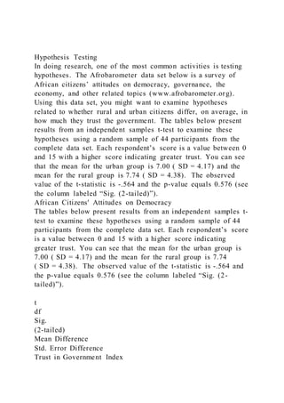
The tables below present results from an independent samples t-test to examine these hypotheses using a random sample of 44 participants from the complete data set. Each respondent’s score is a value between 0 and 15 with a higher score indicating greater trust. You can see that the mean for the urban group is 7.00 ( SD = 4.17) and the mean for the rural group is 7.74 ( SD = 4.38). The observed value of the t-statistic is -.564 and the p-value equals 0.576 (see the column labeled “Sig. (2-tailed)”).
t
df
Sig.
(2-tailed)
Mean Difference
Std. Error Difference
Trust in Government Index
(higher scores = more trust)
-.564
41
.576
-.73913
1.30978
Group Statistics
Urban or Rural Primary
Sampling Unit
N
Mean
Std. Deviation
Std. Error Mean
Trust in Government Index
(higher scores = more trust)
Urban
20
7.000
4.16754
.93189
Rural
30
7.7391
4.38196
.91370
The p-value is the probability of obtaining a value more extreme than .564 (less than -.564 or greater than +.564) if you were to repeat the test with a new sample of data and if the null hypothesis is true. You will see in this Skill Builder that the p-valuecan easily be used to make statistical decisions in hypothesis testing. However, while the p-valueis important in determining statistical significance, it does not tell the whole story.
Steps of Hypothesis Testing
To interpret p-values, let's review the key steps in hypothesis testing. Use the < and > icons to navigate between the steps.
Step 1
State the null and alternative hypotheses
Recall that hypotheses are statements about population parameters. For the Trust in Government example from the Afrobarometer data set, the null (HO) and alternative hypotheses (HA) is seen in the above image.
The Greek letter, µ, indicates a population mean, and the subscripts indicate levels of the independent variable (“urban” and “rural”). Here the null is saying that the mean for the urban population on the Trust In Government variable is the same as the mean for the rural population. The alternative hypothe ...
Hypothesis TestingIn doing research, one of the most common acti
1. Hypothesis Testing
In doing research, one of the most common activities is testing
hypotheses. The Afrobarometer data set below is a survey of
African citizens’ attitudes on democracy, governance, the
economy, and other related topics (www.afrobarometer.org).
Using this data set, you might want to examine hypotheses
related to whether rural and urban citizens differ, on average, in
how much they trust the government. The tables below present
results from an independent samples t-test to examine these
hypotheses using a random sample of 44 participants from the
complete data set. Each respondent’s score is a value between 0
and 15 with a higher score indicating greater trust. You can see
that the mean for the urban group is 7.00 ( SD = 4.17) and the
mean for the rural group is 7.74 ( SD = 4.38). The observed
value of the t-statistic is -.564 and the p-value equals 0.576 (see
the column labeled “Sig. (2-tailed)”).
African Citizens' Attitudes on Democracy
The tables below present results from an independent samples t-
test to examine these hypotheses using a random sample of 44
participants from the complete data set. Each respondent’s score
is a value between 0 and 15 with a higher score indicating
greater trust. You can see that the mean for the urban group is
7.00 ( SD = 4.17) and the mean for the rural group is 7.74
( SD = 4.38). The observed value of the t-statistic is -.564 and
the p-value equals 0.576 (see the column labeled “Sig. (2-
tailed)”).
t
df
Sig.
(2-tailed)
Mean Difference
Std. Error Difference
Trust in Government Index
2. (higher scores = more trust)
-.564
41
.576
-.73913
1.30978
Group Statistics
Urban or Rural Primary
Sampling Unit
N
Mean
Std. Deviation
Std. Error Mean
Trust in Government Index
(higher scores = more trust)
Urban
20
7.000
4.16754
.93189
Rural
30
7.7391
4.38196
.91370
The p-value is the probability of obtaining a value more
extreme than .564 (less than -.564 or greater than +.564) if you
were to repeat the test with a new sample of data and if the null
hypothesis is true. You will see in this Skill Builder that the p-
valuecan easily be used to make statistical decisions in
hypothesis testing. However, while the p-valueis important in
determining statistical significance, it does not tell the whole
story.
Steps of Hypothesis Testing
3. To interpret p-values, let's review the key steps in hypothesis
testing. Use the < and > icons to navigate between the steps.
Step 1
State the null and alternative hypotheses
Recall that hypotheses are statements about population
parameters. For the Trust in Government example from the
Afrobarometer data set, the null (HO) and alternative
hypotheses (HA) is seen in the above image.
The Greek letter, µ, indicates a population mean, and the
subscripts indicate levels of the independent variable (“urban”
and “rural”). Here the null is saying that the mean for the urban
population on the Trust In Government variable is the same as
the mean for the rural population. The alternative hypothesis
states that these means are not the same.
One-tailed vs. Two-tailed Tests
One important factor to be aware of is whether the test you are
conducting is one-tailed or two-tailed. So far, the hypotheses
have been written for a two-tailed test, which means that the
alternative hypothesis stated simply that there was a difference
between the means, without specifying the direction of the
difference. In a one-tailed test, the alternative hypothesis does
specify the direction of the difference; that is, it specifies that
one of the means (e.g., urban or rural) is expected to be larger
than the other.
In a one-tailed test, the p-value will be the area in the test
statistic distribution to the right of the observed value if the
alternative hypothesis has an “is greater than” sign, and to the
left of the observed value if the alternative hypothesis has an
“is less than” sign. For example, suppose we had the following
hypothesis test:
In this hypothesis test, the alternative hypothesis HA states that
the mean for the urban population will be greater than the mean
4. for the rural population. The p-value would, therefore, be
determined by the area to the right of the observed value of the
test statistic using the sampling distribution for the test
statistic.
For a two-tailed test, as is being illustrated with the
Afrobarometer data file, the area beyond the observed value is
doubled to obtain the p-value. The reason for doubling is related
to setting the rejection region for a two-tailed test. For a two-
tailed test, alpha is divided in half (α/2), and the “half-areas”
are used to identify rejection regions in both the upper and
lower tails of the test statistic’s sampling distribution.
The doubling of the area beyond the observed value allows
the p-value to be compared to alpha to test the null hypothesis.
Figure 1
Figure 1 shows the p-value determination for the Afrobarometer
hypothesis test. In the SPSS output, the observed value for
the t-statistic is -0.564. Because the value of t is negative, the
more extreme values of t are considered to be to the left of -
0.564. As shown in Figure 1, the area under the t curve and less
than -0.564 is .288. Because of the two-tailed test, however, the
area is doubled to account for the probability of the test statistic
taking on a value greater than +0.564. Hence the p-value for the
hypothesis test is .576.
Again, if alpha had been set equal to .05, the null hypothesis
would be retained (fail to reject) because .576 is greater than
.05. That is, the data support the position that in the populations
of urban and rural citizens, there is no difference in average
levels of trust in government.
Keep in mind the following important points related to making a
statistical decision and interpreting your p-value:
· bullet
By definition, the p-value is the probability of obtaining a value
for the test statistic as extreme or more extreme than the
observed value if the null hypothesis is true.
· bullet
5. If the p-value is less than alpha, the null is rejected, and the
result is said to be statistically significant.
· bullet
If the p-value is greater than alpha, then researchers would fail
to reject the null hypothesis.
Statistically Significant Results
The final step in conducting a hypothesis test is to link the
statistical result to the real-world. That is, you need to examine
the practical significance or the meaningfulness of the
statistical result.
If the result of the hypothesis test is to retain the null —that is,
obtain a non-significant result—the researcher has clearly not
identified a meaningful effect. In most hypothesis tests,
retaining the null is not what the researcher is hoping to do.
On the other hand, if you reject the null hypothesis, you will
have a statistically significant result. You are, in essence,
saying that the result is so unlikely under the assumption of the
null being true that the null appears to be false. A false null
hypothesis does not mean, however, that the result is
scientifically or socially important. When a researcher finds a
statistically significant result, knowledge of the research area is
used to decide whether the result is important and meaningful.
Large effects are more often meaningful than small effects, but
there are times when small effects can be important.
Knowledge of the research area is key in making the decision.
Probably the most frequent concern with meaningless
statistically significant results has to do with sample size. With
extremely large sample sizes, hypothesis tests can result in
rejecting the null even though the effect is small and
unimportant from an applied perspective. To understand how
this works, let’s take another look at the Afrobarometer data
set. Participants in the survey were asked whether they agreed
or disagreed with the statement, “People must obey the law.”
Responses were made using a five-point Likert scale:
6. 1
2
3
4
5
strongly disagree
disagree
neither agree nor disagree
agree
strongly agree
Suppose a researcher had wanted to compare the urban and rural
populations and tested the null hypothesis
Ho : μurban = μrural using alpha equal to .05. Unlike the
example above that used a sample of 43 participants, the
following results are based on over 50,000 respondents. As
shown in the following table, the p-value ( Sig (2-tailed)) for
this test is .004.
t
df
Sig (2-tailed)
Mean Difference
Q48b. People must obey the law
Equal variances assumed
-.2892
50125
.004
-.029
Using APA style, the researcher could report that, on average,
the urban population agrees less with the statement than does
the rural population, t (50125) = -2.892, p = .004, d = .027,
95% CI [-.039, -.019].
· bullet
The statement says the t-test was conducted with 50,125 degrees
of freedom or 50,127 participants.
7. · bullet
The p-value of .004 is less than alpha, so the null hypothesis is
rejected.
· bullet
The d statistic is Cohen’s d, a common measure of effect size.
· bullet
The 95% confidence interval for the difference in population
means does not contain zero, which is consistent with having
rejected the null hypothesis.
There is no doubt the result is statistically significant, but how
meaningful is it? The d-statistic is quite useful because it
compares the difference in sample means to an average of the
standard deviations for the two groups. (The average standard
deviation is based on a weighted average of the two sample
variances.) According to Cohen, d = .2 is generally considered a
small effect, d = .5 a medium effect, and d = .8 a large effect.
The value of .027 is little more than 10% of a small effect. The
statistically significant result that was obtained is therefore not
likely to be important.
Statistical Power
Statistical power is the probability of rejecting a null hypothesis
if the null is false (i.e., the alternative is true). It is the degree
to which the researcher is able to detect an effect if there
actually is one. With low statistical power, a researcher may
struggle to detect an effect (to reject the null), even if an effect
actually occurs in the population.
Suppose you are planning an experiment involving stereotype
threat. Stereotype threat is defined as a tendency to behave in a
manner consistent with negative beliefs that others have about a
racial or gender group. For example, if some black test takers
are told that as a group, black test takers do not perform well on
math tests, performance among those black test-takers is worse
than for black test takers for whom the stereotype is not evoked.
One question you will need to answer is how many participants
8. should you include in your study to be confident in identifying
the effect? In other words, how many participants do you need
in order to have adequate statistical power in your study?
The Affect of Statistical Power
Understanding how several factors affect the statistical power
of a study will help you to understand and critique research
findings and will also lead to greater satisfaction with your own
research. When conducting your own research studies, you
should do a power analysis prior to collecting data to make sure
you have a good chance of demonstrating the effect you are
looking for.
There are three main factors that affect how much statistical
power you have in your study:
· 1
1
Alpha (i.e., the probability of a type I error)
· 2
2
Effect size (i.e., the difference between the population means
for the experimental and control groups)
· 3
3
Sample size (i.e., n )
As a researcher, you have control over alpha and sample size.
The effect size, however, is not under your control and is
predetermined. What will be important to you is having an idea
about how great the effect may be. This Skill Builder is
concerned with how alpha, effect size, and sample size are
related to statistical power.
A Review of Hypothesis Testing
Before discussing power, let’s review the basics of hypothesis
testing:
· bullet
The null hypothesis is the statement of no effect.
· bullet
The alternative hypothesis is a statement that an effect exists in
9. the population.
· bullet
Obtaining a significant result means that you have rejected the
null hypothesis and have concluded that it’s likely that
there is an effect in the population.
· bullet
A type I error happens when the null hypothesis is true but you
reject it erroneously. This is referred to as a false positive.
· bullet
A type II error happens when the null hypothesis is false but
you fail to reject it. This is referred to as a false negative.
Reviewing Type I and Type II Errors
Type I and type II errors and their probabilities are important
concepts when thinking about hypothesis testing. These error
events are called “conditional,” meaning that the events can
only occur under certain conditions.
The following is the language that is used to talk about these
conditional events:
· Alpha (α) = P(type I error) = P(Reject H 0 |H 0 is true) which
is read as the probability of a type I error equals the probability
of rejecting the null hypothesis given the null is true.
· Beta (β) = P(type II error) = P(Retain H 0 |H A is true) which
is read as the probability of a type II error equals the
probability of retaining the null hypothesis given the alternative
hypothesis is true.
Table 1 shows the possible outcomes for a hypothesis test.
Table 1: Possible Outcomes for a Hypothesis Test
D
True State of Nature
Decision
Ho is true
Ho is false
Retain Ho
Correct decision
Type II error
Reject Ho
10. Type 1 error
Correct decision
Power Analysis
Power analysis is the process of examining a test of the null
hypothesis to determine the chances of rejecting it and placing
belief in the alternative hypothesis.
Researchers typically want to get a sense of how much
statistical power they will have in their study before coll ecting
data. In order to do so, they usually conduct a power analysis.
Suppose you design a study, and a part of it is to demonstrate
stereotype threat involving females. Nguyen and Ryan (2008)
provide results that indicate the average Cohen’s d in previous
studies of gender-based stereotype threat for cognitive tests is
about .21. This means that over many studies, females who are
NOT made aware of a gender stereotype (NOT primed) score
about 0.2 standard deviations higher on cognitive tests than
females who are made aware of a gender effect (primed). To
demonstrate this effect in your study, you will test the
following null hypothesis:
HA : μNOT primed − μprimed ≤ 0
If you reject the null, you will place your confidence in the
following alternative hypothesis:
HA : μNOT primed − μprimed > 0
μNOT primed
Indicates the population mean for the “not primed” condition.
μprimed
Indicates the population mean for the “primed” condition.
HA : μNOT primed − μprimed > 0
The alternative hypothesis specifies that the “not primed”
condition will score higher than the “primed” condition.
To test this null hypothesis, you would examine a test statistic
distribution and note the area in the upper tail of the
distribution equal to alpha. Suppose you plan to test this
hypothesis with a t-test with 50 participants in each condition
(primed or NOT primed).
11. Figure 1 sampling distribution shows what you should expect
for the values of the test statistic if the null hypothesis is true.
In order to reject the null hypothesis, the t value would need to
be greater than 1.66055.
Figure 1
Because the test statistic is a continuous variable, the curve
shows probability density, and probability is found by
determining the area under the curve.
The entire area under the curve, between - ∞and+ ∞, is 1.00.
To find the probability of a statistic taking on a value within a
certain range, you need to find the area under the curve within
the range. For example, there are tables that will tell you that
the area under the curve between t = 0 and t = +1 corresponds to
a probability of about .34. Most importantly, because alpha has
been set equal to .05, the area beyond 1.66 corresponds to a
probability of .05. Fortunately, statistical programs calculate
the areas for you, and you do not need to do the calculations
yourself.
Nevertheless, the essence of hypothesis testing is that if you
obtain a value of t greater than 1.66, you will say, “This is not a
very likely event if the null is true. Thus, the null hypothesis is
probably not true because the alternative hypothesis provides a
more likely explanation.” In making the decision to reject the
null, however, you recognize that if the null is, in fact, true, you
are making a type I error.
While alpha provides assurance that the researcher has a small
chance of making a type I error, you are also interested in what
will happen if the null hypothesis is false—the real world
expectation that is driving you to do the study.
Figure 2
Now, in Figure 2, switch your focus from the curve on the left
and attend to the curve on the right formed by the dashed line.
This curve is based on the alternative hypothesis (i.e., that the
unprimed group performs better than the primed group).
12. To construct this curve based on the alternative hypothesis, a
specific value for the difference in means had to be specified; in
this case, the value of d = .21, the overall gender effect that
Nguyen and Ryan (2008) found. Note, again, that the vertical
line with t = 1.66 separates the values of the test statistic that
lead to rejecting versus retaining the null hypothesis, and that
the line is based on the null hypothesis. The statistical power of
the test, (1-β), is the area under the curve with the dashed lines
and to the right of the vertical line for t = 1.69. The area
designated by beta (β), to the left of the vertical line,
corresponds to the probability of a type II error, retaining the
null if the null is actually false.
In this example, note that the area corresponding to power (1-β)
is less than the area corresponding to β. Hence, you can
conclude that the power is less than 0.5 because the sum of the
two areas is 1.0. Almost always, you would like statistical
power to be greater than beta for the important hypothesis tests
in your study. In this example, a plan to do an experiment with
50 participants in each group may be doomed. The statistical
power of the test (.27) is relatively low, and the risk of making
a type II error is relatively high. In other words, the statistical
power of the test, as currently constructed, limits your ability to
detect a gender effect of priming versus not priming if there is
one.
Numbered divider 1
Consider the following scenario when answering the question
below.
You are planning a study of stereotype threat and are concerned
you may not be able to detect a significant result, even though
you believe your experimental procedures should induce the
stereotype threat effect.
Hint: A type I error happens when the null hypothesis is true
and you reject it.
Which of the following errors are you concerned about?
Type I error
Type II error
13. TAKE AGAIN
The Relationship Between Power and Sample Size
Prior discussions have focused on testing hypotheses about
population means, but you can also do hypothesis tests
involving population proportions. In general, larger sample
sizes give you more information to pin down the true nature of
the population. You can, therefore, expect the sample mean
and sample proportion obtained from a larger sample to be
closer to the population mean and proportion, respectively.
As a result, for the same level of confidence, you can report a
smaller margin of error, and get a narrower confidence interval.
In other words, larger sample sizes increase how much you trust
your sample results. In the two scenarios below, you will see
that a larger sample size results in a greater ability to reject the
null when an effect actually exists in the population.
Scenario: Examining Marijuana Use
Imagine you are a researcher examining marijuana use at a
certain liberal arts college and read through the scenario below.
Step 1
You believe that marijuana use at the college is greater than the
national average, for which large-scale studies have shown that
about 15.7% of college students use marijuana (reported by the
Harvard School of Public Health). Based on this belief, you
perform the hypothesis test shown in Figure 9 below.
· Note that p in this figure means population proportion
and pˆ means sample proportion. On the other hand, p-value
continues to have the same meaning as defined in the glossary.
Because the p-value is greater than .05, the customary alpha
level, the data do not provide enough evidence that the
proportion of marijuana users at the college is higher than the
proportion among all U.S. college students, which is .157.
Step 2
Let’s make some small changes to the above problem. Suppose
that in a simple random sample of 400 students from the
14. college, 76 admitted to marijuana use as seen in Figure 8 below.
Do the data provide enough evidence to conclude that the
proportion of marijuana users among the students in the college
(p) is higher than the national proportion, which is .157?
Step 3
You now have a larger sample (400 instead of 100), and also the
number of marijuana users is 76 instead of 19. The question of
interest did not change, so if you carry out the test in this case,
you are testing the same hypotheses seen below.
Step 4
You select a random sample of size 400 and find that 76 are
marijuana users, and the formula seen below. This is the same
sample proportion as in the original problem, so it seems that
the data give the same evidence.
Step 5
However, when you calculate the test statistic, you see that
actually this is not the case as seen in the formula below.
Even though the sample proportion is the same (.19), because
here it is based on a larger sample (400 instead of 100), it is
1.81 standard deviations above the null value of .157 (as
opposed to .91 standard deviations in the original problem). The
sampling distribution for the sample proportion has a smaller
standard error because of the larger sample size.
Step 6
The p-value here is .035, as opposed to .182 in the original
problem. In other words, when Ho is true (i.e., if p = .157 at the
certain college), it is quite unlikely (probability of .035) to get
a sample proportion of .19 or higher based on a sample of size
400. When the sample size is 100, the probability of having a
sample proportion greater than .19 is more likely (probability
.182).
15. The results here are important. With n = 400, the data provide
enough evidence to reject Ho and conclude that the proportion
of marijuana users at the college is higher than among all U.S.
students. With n = 100, however, the evidence is insufficient to
reject the null. Figure 9 summarizes these findings.
You can see that results that are based on a larger sample carry
more weight. A sample proportion of .19 based on a sample of
size of 100 was not enough evidence that the proportion of
marijuana users in the college is higher than .157. Recall that
this conclusion (not having enough evidence to reject the null
hypothesis) doesn't mean the null hypothesis is necessarily true;
it only means that the particular study did not yield sufficient
evidence to reject the null. It might be that the sample size was
simply too small to detect a statistically significant difference,
and a type II error was made.
To summarize, you saw that when the sample proportion of .19
is obtained from a sample of size 400, it carries much more
weight, and in particular, provides enough evidence that the
proportion of marijuana users in the college is higher than .157
(the national figure). In this case, the sample size of
400 was large enough to detect a statistically significant
difference.
The following graphs show the power of the two tests if the
population mean proportion p for the certain college is actually
.19. Use the < and > icon to navigate between slides.
· 1
· 2
Figure 10
Figure 11
17. classes offered at
the same university (n = 69). Students reported their level of
satisfaction on a five-
point scale, with higher values indicating higher levels of
satisfaction. Since the
study was exploratory in nature, levels of significance were
relaxed to the .10 level.
The test was significant t(132) = 1.8, p = .074, wherein students
in the face-to-face
class reported lower levels of satisfaction (M = 3.39, SD = 1.8)
than did those in the
online sections (M = 3.89, SD = 1.4). We therefore conclude
that on average,
students in online quantitative reasoning classes have higher
levels of satisfaction.
The results of this study are significant because they provide
educators with
evidence of what medium works better in producing
quantitatively knowledgeable
practitioners.
2. A results report that does not find any effect and also has
small sample size
(possibly no effect detected due to lack of power).
A one-way analysis of variance was used to test whether a
relationship exists
between educational attainment and race. The dependent
variable of education
was measured as number of years of education completed. The
race factor had
three attributes of European American (n = 36), African
American (n = 23) and
Hispanic (n = 18). Descriptive statistics indicate that on
average, European
Americans have higher levels of education (M = 16.4, SD =
19. levels of cultural competency. The descriptive statistics indicate
women have
higher levels of cultural competency (M = 9.2, SD = 3.2) than
men (M = 8.9, SD =
2.1). The results were significant t (1311) = 2.0, p <.05,
indicating that women are
more culturally competent than are men. These results tell us
that gender-specific
interventions targeted toward men may assist in bolstering
cultural competency.
4. A study has results that seem fine, but there is no clear
association to social
change. What is missing?
A correlation test was conducted to determine whether a
relationship exists
between level of income and job satisfaction. The sample
consisted of 432
employees equally represented across public, private, and non-
profit sectors. The
results of the test demonstrate a strong positive correlation
between the two
variables, r =.87, p < .01, showing that as level of income
increases, job
satisfaction increases as well.
Assignment: Evaluating Significance of Findings
Part of your task as a scholar-practitioner is to act as a critical
consumer of research and ask informed questions of published
material. Sometimes, claims are made that do not match the
results of the analysis. Unfortunately, this is why statistics is
sometimes unfairly associated with telling lies. These
misalignments might not be solely attributable to statistical
20. nonsense, but also “user error.” One of the greatest areas of user
error is within the practice of hypothesis testing and
interpreting statistical significance. As you continue to consume
research, be sure and read everything with a critical eye and call
out statements that do not match the results.
For this Assignment, you will examine statistical significance
and meaningfulness based on sample statements.
To prepare for this Assignment:
· Review the Week 5 Scenarios found in this week’s Learning
Resources and select two of the four scenarios for this
Assignment.
· For additional support, review the Skill Builder: Evaluating P
Values and the Skill Builder: Statistical Power, which you can
find by navigating back to your Blackboard Course Home Page.
From there, locate the Skill Builder link in the left navigation
pane.
For this Assignment:
Critically evaluate the two scenarios you selected based upon
the following points:
· Critically evaluate the sample size.
· Critically evaluate the statements for meaningfulness.
· Critically evaluate the statements for statistical significance.
· Based on your evaluation, provide an explanation of the
implications for social change.
Use proper APA format and citations, and referencing.
https://www.amstat.org/asa/files/pdfs/p-valuestatement.pdf
Frankfort-Nachmias, C., Leon-Guerrero, A., & Davis, G.
(2020). Social statistics for a diverse society (9th ed.).
Thousand Oaks, CA: Sage Publications.
· Chapter 8, “Testing Hypothesis: Assumptions of Statistical
Hypothesis Testing” (pp. 241-242)
21. Wagner, III, W. E. (2020). Using IBM® SPSS® statistics for
research methods and social science statistics (7th ed.) .
Thousand Oaks, CA: Sage Publications.
· Chapter 6, “Testing Hypotheses Using Means and Cross-
Tabulation”
https://content.waldenu.edu/content/dam/laureate/laureate-
academics/wal/xx-rsch/rsch-
8210/readings/USW1_RSCH_8210_Week05_Warner_chapter03.
pdf
Walden University, LLC. (Producer). (2016f). Meaningfulness
vs. statistical significance [Video file]. Baltimore, MD: Author.
Note: The approximate length of this media piece is 4 minutes.
In this media program, Dr. Matt Jones discusses the differences
in meaningfulness and statistical significance. Focus on how
this information will inform your Discussion and Assignment
for this week.
Skill builder: Evaluating P Values
Hypothesis Testing
In doing research, one of the most common activities is testing
hypotheses. The Afrobarometer data set below is a survey of
African citizens’ attitudes on democracy, governance, the
economy, and other related topics (www.afrobarometer.org).
Using this data set, you might want to examine hypotheses
related to whether rural and urban citizens differ, on average, in
how much they trust the government. The tables below present
results from an independent samples t-test to examine these
hypotheses using a random sample of 44 participants from the
22. complete data set. Each respondent’s score is a value between 0
and 15 with a higher score indicating greater trust. You can see
that the mean for the urban group is 7.00 ( SD = 4.17) and the
mean for the rural group is 7.74 ( SD = 4.38). The observed
value of the t-statistic is -.564 and the p-value equals 0.576 (see
the column labeled “Sig. (2-tailed)”).
African Citizens' Attitudes on Democracy
The tables below present results from an independent samples t-
test to examine these hypotheses using a random sample of 44
participants from the complete data set. Each respondent’s score
is a value between 0 and 15 with a higher score indicating
greater trust. You can see that the mean for the urban group is
7.00 ( SD = 4.17) and the mean for the rural group is 7.74
( SD = 4.38). The observed value of the t-statistic is -.564 and
the p-value equals 0.576 (see the column labeled “Sig. (2-
tailed)”).
t
df
Sig.
(2-tailed)
Mean Difference
Std. Error Difference
Trust in Government Index
(higher scores = more trust)
-.564
41
.576
-.73913
1.30978
Group Statistics
Urban or Rural Primary
Sampling Unit
N
Mean
23. Std. Deviation
Std. Error Mean
Trust in Government Index
(higher scores = more trust)
Urban
20
7.000
4.16754
.93189
Rural
30
7.7391
4.38196
.91370
The p-value is the probability of obtaining a value more
extreme than .564 (less than -.564 or greater than +.564) if you
were to repeat the test with a new sample of data and if the null
hypothesis is true. You will see in this Skill Builder that the p-
valuecan easily be used to make statistical decisions in
hypothesis testing. However, while the p-valueis important in
determining statistical significance, it does not tell the whole
story.
Steps of Hypothesis Testing
To interpret p-values, let's review the key steps in hypothesis
testing. Use the < and > icons to navigate between the steps.
Step 1
State the null and alternative hypotheses
Recall that hypotheses are statements about population
parameters. For the Trust in Government example from the
Afrobarometer data set, the null (HO) and alternative
hypotheses (HA) is seen in the above image.
The Greek letter, µ, indicates a population mean, and the
subscripts indicate levels of the independent variable (“urban”
and “rural”). Here the null is saying that the mean for the urban
24. population on the Trust In Government variable is the same as
the mean for the rural population. The alternative hypothesis
states that these means are not the same.
Step 2
Set alpha , the probability of a type I error
Frequently, the value of alpha is set equal to 0.05, although
researchers are free to use other values. If using an alpha of .05,
then researchers are specifying that there is a 5% chance that
they will reject the null when, in fact, it should not be rejected.
Setting alpha at .05 is popular because there is relatively
minimal risk of making a type I error, and alpha is not so small
that researchers greatly increase their risk of not rejecting the
null when they actually should (a type II error). So in setting
alpha, researchers have to be aware of both the risk of r ejecting
the null erroneously and of not rejecting it when they actually
should. For our Afrobarometer example, we will set alpha at
.05.
Step 1
State the null and alternative hypotheses
Recall that hypotheses are statements about population
parameters. For the Trust in Government example from the
Afrobarometer data set, the null (HO) and alternative
hypotheses (HA) is seen in the above image.
The Greek letter, µ, indicates a population mean, and the
subscripts indicate levels of the independent variabl e (“urban”
and “rural”). Here the null is saying that the mean for the urban
population on the Trust In Government variable is the same as
the mean for the rural population. The alternative hypothesis
states that these means are not the same.
Step 2
Set alpha , the probability of a type I error
25. Frequently, the value of alpha is set equal to 0.05, although
researchers are free to use other values. If using an alpha of .05,
then researchers are specifying that there is a 5% chance that
they will reject the null when, in fact, it should not be rejected.
Setting alpha at .05 is popular because there is relatively
minimal risk of making a type I error, and alpha is not so small
that researchers greatly increase their risk of not rejecting the
null when they actually should (a type II error). So in setting
alpha, researchers have to be aware of both the risk of rejecting
the null erroneously and of not rejecting it when they actually
should. For our Afrobarometer example, we will set alpha at
.05.
Step 3
Decide on a test statistic
Because of a desire to compare two groups (rural and urban),
a t-test for two independent samples is being used.
Step 1
State the null and alternative hypotheses
Recall that hypotheses are statements about population
parameters. For the Trust in Government example from the
Afrobarometer data set, the null (HO) and alternative
hypotheses (HA) is seen in the above image.
The Greek letter, µ, indicates a population mean, and the
subscripts indicate levels of the independent variable (“urban”
and “rural”). Here the null is saying that the mean for the urban
population on the Trust In Government variable is the same as
the mean for the rural population. The alternative hypothesis
states that these means are not the same.
Step 2
Set alpha , the probability of a type I error
Frequently, the value of alpha is set equal to 0.05, although
researchers are free to use other values. If using an alpha of .05,
26. then researchers are specifying that there is a 5% chance that
they will reject the null when, in fact, it should not be rejected.
Setting alpha at .05 is popular because there is relatively
minimal risk of making a type I error, and alpha is not so small
that researchers greatly increase their risk of not rejecting the
null when they actually should (a type II error). So in setting
alpha, researchers have to be aware of both the risk of rejecting
the null erroneously and of not rejecting it when they actually
should. For our Afrobarometer example, we will set alpha at
.05.
Step 3
Decide on a test statistic
Because of a desire to compare two groups (rural and urban),
a t-test for two independent samples is being used.
7
Step 4
Collect the data and examine the model assumptions
Before calculating the value for your test statistic, be sure you
have checked assumptions, like homogeneity of variance and
the absence of outliers.
Step 5
Calculate the observed value of the test statistic
Once the data have been collected, the observed value of the
test statistic will be used to make a statistical decision. In the
Afrobarometer example, the observed value of the test statistic
is -.564, sometimes written as tobserved(41)= −.564 where the
41 is the number of degrees of freedom associated with the test.
Step 1
State the null and alternative hypotheses
Recall that hypotheses are statements about population
parameters. For the Trust in Government example from the
27. Afrobarometer data set, the null (HO) and alternative
hypotheses (HA) is seen in the above image.
The Greek letter, µ, indicates a population mean, and the
subscripts indicate levels of the independent variable (“urban”
and “rural”). Here the null is saying that the mean for the urban
population on the Trust In Government variable is the same as
the mean for the rural population. The alternative hypothesis
states that these means are not the same.
Step 2
Set alpha , the probability of a type I error
Frequently, the value of alpha is set equal to 0.05, although
researchers are free to use other values. If using an alpha of .05,
then researchers are specifying that there is a 5% chance that
they will reject the null when, in fact, it should not be rejected.
Setting alpha at .05 is popular because there is relatively
minimal risk of making a type I error, and alpha is not so small
that researchers greatly increase their risk of not rejecting the
null when they actually should (a type II error). So in setting
alpha, researchers have to be aware of both the risk of rejecting
the null erroneously and of not rejecting it when they actually
should. For our Afrobarometer example, we will set alpha at
.05.
Step 3
Decide on a test statistic
Because of a desire to compare two groups (rural and urban),
a t-test for two independent samples is being used.
Step 4
Collect the data and examine the model assumptions
Before calculating the value for your test statistic, be sure you
have checked assumptions, like homogeneity of variance and
the absence of outliers.
Step 5
Calculate the observed value of the test statistic
Once the data have been collected, the observed value of the
test statistic will be used to make a statistical decision. In the
Afrobarometer example, the observed value of the test statistic
28. is -.564, sometimes written as tobserved(41)= −.564 where the
41 is the number of degrees of freedom associated with the test.
Step 6
Make a statistical decision using the observed value
This decision requires examining the distribution of the test
statistic under the assumption the null hypothesis is true.
Practically, the area in the tail of the distribution beyond the
observed value of the test statistic, called the p-value, needs to
be determined (see the figure above). Fortunately, computer
programs can do the calculation of the area quickly and easily.
If the probability is less than alpha (e.g., .05), we will reje ct the
null hypothesis. Thus, if you set alpha equal to .05 and the p-
value for your test statistic is any value less than .05, you will
reject the null hypothesis. Otherwise, retain the null.
Step 7
Make a real-world decision
The statistical decision is focused on the abstract hypothesis
test. The final step is to examine the implications of the
statistical decision in the real world. You will need to consider
whether your results are practically significant. It turns out that
not all statistically significant results are important in the real
world. We will discuss more about this later in the Skill
Builder.
Skill Builder: Statistical Power,
Statistical Power
Statistical power is the probability of rejecting a null hypothesis
if the null is false (i.e., the alternative is true). It is the degree
to which the researcher is able to detect an effect if there
actually is one. With low statistical power, a researcher may
struggle to detect an effect (to reject the null), even if an effect
actually occurs in the population.
29. Suppose you are planning an experiment involving stereotype
threat. Stereotype threat is defined as a tendency to behave in a
manner consistent with negative beliefs that others have about a
racial or gender group. For example, if some black test takers
are told that as a group, black test takers do not perform well on
math tests, performance among those black test-takers is worse
than for black test takers for whom the stereotype is not evoked.
One question you will need to answer is how many participants
should you include in your study to be confident in identifying
the effect? In other words, how many participants do you need
in order to have adequate statistical power in your study?
The Affect of Statistical Power
Understanding how several factors affect the statistical power
of a study will help you to understand and critique research
findings and will also lead to greater satisfaction with your own
research. When conducting your own research studies, you
should do a power analysis prior to collecting data to make sure
you have a good chance of demonstrating the effect you are
looking for.
There are three main factors that affect how much statistical
power you have in your study:
· 1
1
Alpha (i.e., the probability of a type I error)
· 2
2
Effect size (i.e., the difference between the population means
for the experimental and control groups)
· 3
3
Sample size (i.e., n )
As a researcher, you have control over alpha and sample size.
The effect size, however, is not under your control and is
predetermined. What will be important to you is having an idea
about how great the effect may be. This Skill Builder is
concerned with how alpha, effect size, and sample size are
30. related to statistical power.
A Review of Hypothesis Testing
Before discussing power, let’s review the basics of hypothesis
testing:
· bullet
The null hypothesis is the statement of no effect.
· bullet
The alternative hypothesis is a statement that an effect exists in
the population.
· bullet
Obtaining a significant result means that you have rejected the
null hypothesis and have concluded that it’s likely that
there is an effect in the population.
· bullet
A type I error happens when the null hypothesis is true but you
reject it erroneously. This is referred to as a false positive.
· bullet
A type II error happens when the null hypothesis is false but
you fail to reject it. This is referred to as a false negative.
Reviewing Type I and Type II Errors
Type I and type II errors and their probabilities are important
concepts when thinking about hypothesis testing. These error
events are called “conditional,” meaning that the events can
only occur under certain conditions.
The following is the language that is used to talk about these
conditional events:
· Alpha (α) = P(type I error) = P(Reject H 0 |H 0 is true) which
is read as the probability of a type I error equals the probability
of rejecting the null hypothesis given the null is true.
· Beta (β) = P(type II error) = P(Retain H 0 |H A is true) which
is read as the probability of a type II error equals the
probability of retaining the null hypothesis given the alternative
hypothesis is true.
Table 1 shows the possible outcomes for a hypothesis test.
31. Table 1: Possible Outcomes for a Hypothesis Test
D
True State of Nature
Decision
Ho is true
Ho is false
Retain Ho
Correct decision
Type II error
Reject Ho
Type 1 error
Correct decision
Power Analysis
Power analysis is the process of examining a test of the null
hypothesis to determine the chances of rejecting it and placing
belief in the alternative hypothesis.
Researchers typically want to get a sense of how much
statistical power they will have in their study before collecting
data. In order to do so, they usually conduct a power analysis.
Suppose you design a study, and a part of it is to demonstrate
stereotype threat involving females. Nguyen and Ryan (2008)
provide results that indicate the average Cohen’s d in previous
studies of gender-based stereotype threat for cognitive tests is
about .21. This means that over many studies, females who are
NOT made aware of a gender stereotype (NOT primed) score
about 0.2 standard deviations higher on cognitive tests than
females who are made aware of a gender effect (primed). To
demonstrate this effect in your study, you will test the
following null hypothesis:
HA : μNOT primed − μprimed ≤ 0
If you reject the null, you will place your confidence in the
following alternative hypothesis:
HA : μNOT primed − μprimed > 0
μNOT primed
Indicates the population mean for the “not primed” condition.
32. μprimed
Indicates the population mean for the “primed” condition.
HA : μNOT primed − μprimed > 0
The alternative hypothesis specifies that the “not primed”
condition will score higher than the “primed” condition.
To test this null hypothesis, you would examine a test statistic
distribution and note the area in the upper tail of the
distribution equal to alpha. Suppose you plan to test this
hypothesis with a t-test with 50 participants in each condition
(primed or NOT primed).
Figure 1 sampling distribution shows what you should expect
for the values of the test statistic if the null hypothesis is true.
In order to reject the null hypothesis, the t value would need to
be greater than 1.66055.
Figure 1
Because the test statistic is a continuous variable, the cur ve
shows probability density, and probability is found by
determining the area under the curve.
The entire area under the curve, between - ∞and+ ∞, is 1.00.
To find the probability of a statistic taking on a value within a
certain range, you need to find the area under the curve within
the range. For example, there are tables that will tell you that
the area under the curve between t = 0 and t = +1 corresponds to
a probability of about .34. Most importantly, because alpha has
been set equal to .05, the area beyond 1.66 corresponds to a
probability of .05. Fortunately, statistical programs calculate
the areas for you, and you do not need to do the calculations
yourself.
Nevertheless, the essence of hypothesis testing is that if you
obtain a value of t greater than 1.66, you will say, “This is not a
very likely event if the null is true. Thus, the null hypothesis is
probably not true because the alternative hypothesis provides a
more likely explanation.” In making the decision to reject the
null, however, you recognize that if the null is, in fact, true, you
are making a type I error.
33. While alpha provides assurance that the researcher has a small
chance of making a type I error, you are also interested in what
will happen if the null hypothesis is false—the real world
expectation that is driving you to do the study.
Figure 2
Now, in Figure 2, switch your focus from the curve on the left
and attend to the curve on the right formed by the dashed line.
This curve is based on the alternative hypothesis (i.e., that the
unprimed group performs better than the primed group).
To construct this curve based on the alternative hypothesis, a
specific value for the difference in means had to be specified; in
this case, the value of d = .21, the overall gender effect that
Nguyen and Ryan (2008) found. Note, again, that the vertical
line with t = 1.66 separates the values of the test statistic that
lead to rejecting versus retaining the null hypothesis, and that
the line is based on the null hypothesis. The statistical power of
the test, (1-β), is the area under the curve with the dashed lines
and to the right of the vertical line for t = 1.69. The area
designated by beta (β), to the left of the vertical line,
corresponds to the probability of a type II error, retaining the
null if the null is actually false.
In this example, note that the area corresponding to power (1-β)
is less than the area corresponding to β. Hence, you can
conclude that the power is less than 0.5 because the sum of the
two areas is 1.0. Almost always, you would like statistical
power to be greater than beta for the important hypothesis tests
in your study. In this example, a plan to do an experiment with
50 participants in each group may be doomed. The statistical
power of the test (.27) is relatively low, and the risk of making
a type II error is relatively high. In other words, the statistical
power of the test, as currently constructed, limits your ability to
detect a gender effect of priming versus not priming if there is
one.
Power Analysis
34. As the researcher, you have control of alpha, and you will set
alpha when you are planning your study. Continuing with the
example from the previous page, Figure 4 below shows what
would happen to power if you change alpha, the probability of a
type I error, to .15.
Figure 2
Figure 2
Compare the curves in Figure 3 to the ones above in Figure 2; in
that figure, alpha (α) was equal to .05. Notice that β becomes
smaller, and power, (1-β), becomes larger. If you change α to
.01, a relatively small value for the probability of a type I error,
beta (β) becomes larger, and power becomes less. See Figure 4
below.
Figure 3
Figure 3
Figure 4
Figure 4
· bullet
In general, making alpha (α) smaller results in a decrease in the
power of the statistical test, and making alpha larger results in
greater power. This is because if you set a more stringent alpha
(e.g., .01 instead of .05), it becomes more difficult to reject the
null hypothesis. While .05 is a typical value for α, the decision
of which value to use for α is up to the researcher. Letting alpha
(α) equal .05 is certainly common practice.
· bullet
Many journal editors expect alpha (α) to equal .05. There are
other times, however, when the researcher may wish to use a
different value for alpha (α) depending on the severity of the
consequences for making a type I error. For example, if you are
studying whether or not a drug has serious side effects, with the
null specifying that there are no serious side effects, you may
35. want to have a more stringent alpha to lower your risk of saying
that there aren’t side effects when there actually are; you may
opt for a .01 alpha instead of a .05 alpha.
Power and Effect Size
A second factor that is related to the statistical power of a test
is the effect size. There are several measures of effect size.
With a comparison of two populations, Cohen’s d is often used.
The value of d is the difference in population means between
two groups in standard deviation units. According to Cohen’s
rule of thumb, a value of d = .2 is considered a small effect, d =
.5 is considered a medium sized effect, and d = .8 is considered
a large effect.
Let’s revisit the earlier example about planning a study to
demonstrate race-based stereotype threat. Nguyen and Ryan
(2008) note that overall race-based stereotype threat studies
have resulted in an average d equal to about .32. Figure 5 below
shows what you can expect if you induced a general racial
stereotype threat in a rather typical way so that in the
population d = .32, there are 50 participants in each group, and
alpha = .05. Note that power has increased noticeably compared
to the study examined in Figure 2. This is due to the effect size
( d = .32) in this figure being larger than the effect size ( d =
.21) in Figure 2.
Figure 5
Figure 5
There are instances in which stereotype effects as large as d =
.64 have been identified in the samples being studied. If the
population d is .64, the hypothesis test with alpha = .05 and 50
participants in each group will result in power equal to .93 as
shown in Figure 6. This is a high value for statistical power,
meaning that the researchers are very likely to detect an effect
if d = .64 in the population.
Figure 6
36. Figure 6
Most researchers prefer to have the estimate of power be at least
.80 before they are willing to conduct a study. So planning to do
a study with 50 participants in each group may be a bad
decision if the effect size in the population is small or
moderate, as it was above in Figures 2 and 5. On the other hand,
with a large effect (e.g., d = .64), a sample of 50 participants in
each condition provides more than sufficient statistical power
for most researchers.
The Relationship Between Power and Sample Size
Prior discussions have focused on testing hypotheses about
population means, but you can also do hypothesis tests
involving population proportions. In general, larger sample
sizes give you more information to pin down the true nature of
the population. You can, therefore, expect the sample mean
and sample proportion obtained from a larger sample to be
closer to the population mean and proportion, respectively.
As a result, for the same level of confidence, you can report a
smaller margin of error, and get a narrower confidence interval.
In other words, larger sample sizes increase how much you trust
your sample results. In the two scenarios below, you will see
that a larger sample size results in a greater ability to reject the
null when an effect actually exists in the population.
Scenario: Examining Marijuana Use
Imagine you are a researcher examining marijuana use at a
certain liberal arts college and read through the scenario below.
Step 1
You believe that marijuana use at the college is greater than the
national average, for which large-scale studies have shown that
about 15.7% of college students use marijuana (reported by the
Harvard School of Public Health). Based on this belief, you
perform the hypothesis test shown in Figure 9 below.
· Note that p in this figure means population proportion
37. and pˆ means sample proportion. On the other hand, p-value
continues to have the same meaning as defined in the glossary.
Because the p-value is greater than .05, the customary alpha
level, the data do not provide enough evidence that the
proportion of marijuana users at the college is higher than the
proportion among all U.S. college students, which is .157.
Step 2
Let’s make some small changes to the above problem. Suppose
that in a simple random sample of 400 students from the
college, 76 admitted to marijuana use as seen in Figure 8 below.
Do the data provide enough evidence to conclude that the
proportion of marijuana users among the students in the college
(p) is higher than the national proportion, which is .157?
Step 3
You now have a larger sample (400 instead of 100), and also the
number of marijuana users is 76 instead of 19. The question of
interest did not change, so if you carry out the test in this case,
you are testing the same hypotheses seen below.
Step 4
You select a random sample of size 400 and find that 76 are
marijuana users, and the formula seen below. This is the same
sample proportion as in the original problem, so it seems that
the data give the same evidence.
Step 5
However, when you calculate the test statistic, you see that
actually this is not the case as seen in the formula below.
Even though the sample proportion is the same (.19), because
here it is based on a larger sample (400 instead of 100), it is
1.81 standard deviations above the null value of .157 (as
opposed to .91 standard deviations in the original problem). The
sampling distribution for the sample proportion has a smaller
38. standard error because of the larger sample size.
Step 6
The p-value here is .035, as opposed to .182 in the original
problem. In other words, when Ho is true (i.e., if p = .157 at the
certain college), it is quite unlikely (probability of .035) to get
a sample proportion of .19 or higher based on a sample of size
400. When the sample size is 100, the probability of having a
sample proportion greater than .19 is more likely (probability
.182).
The results here are important. With n = 400, the data provide
enough evidence to reject Ho and conclude that the proportion
of marijuana users at the college is higher than among all U.S.
students. With n = 100, however, the evidence is insufficie nt to
reject the null. Figure 9 summarizes these findings.
You can see that results that are based on a larger sample carry
more weight. A sample proportion of .19 based on a sample of
size of 100 was not enough evidence that the proportion of
marijuana users in the college is higher than .157. Recall that
this conclusion (not having enough evidence to reject the null
hypothesis) doesn't mean the null hypothesis is necessarily true;
it only means that the particular study did not yield sufficient
evidence to reject the null. It might be that the sample size was
simply too small to detect a statistically significant difference,
and a type II error was made.
To summarize, you saw that when the sample proportion of .19
is obtained from a sample of size 400, it carries much more
weight, and in particular, provides enough evidence that the
proportion of marijuana users in the college is higher than .157
(the national figure). In this case, the sample size of
400 was large enough to detect a statistically significant
difference.
The following graphs show the power of the two tests if the
population mean proportion p for the certain college is actually
39. .19. Use the < and > icon to navigate between slides.
· 1
· 2
Figure 10
Figure 11
Figure 12
Finally, Figure 12 shows how sample size affects the test for
proportions concerning marijuana use at the liberal arts college.
The graph is based on a hypothesis test with alpha = .05, the
proportion for the null hypothesis equal to .157, and the
population proportion for the liberal arts college = .19.
In general, whether you are testing hypotheses about
proportions, means, or other parameters, the larger the sample
size, the greater the statistical power. Because of your interest
in rejecting the null, you need to pay attention to how large
your sample size will be prior to collecting data.