PRESENTATION ON COST OF PRODUCTION

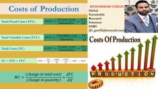
1. MUHAMMAD USMAN
Global
Sustainable
Research
Solutions
GSRS
(E: gsrs92@hotmail.com)
Costs of Production
Fixed cost
Quantity
FC
AFC
Q
= =
Variable cost
Quantity
VC
AVC
Q
= =
Total cost
Quantity
TC
ATC
Q
= =
𝑀𝐶 =
ሺchange in total cost)
ሺchange in quantity)
=
𝛥𝑇𝐶
𝛥𝑄
Total Fixed Costs (TFC)
Total Variable Costs (TVC)
Total Costs (TC)
TC = TFC + TVC

2. Costs as Opportunity Costs
• A firm’s cost of production includes all the opportunity costs of making its output of goods and services.
• A firm’s cost of production include explicit costs and implicit costs.
• Explicit Costs
• Explicit costs are input costs that require a direct outlay of money by the firm.
• A firm’s explicit costs are the monetary payments (or cash expenditures) it makes to those who
supply labor services, materials, fuel, transportation services, and the like. Such money payments
are for the use of resources owned by others.
• Implicit Costs
• Implicit costs are input costs that do not require an outlay of money by the firm.
• A firm’s implicit costs are the opportunity costs of using its self-owned, self-employed resources. To the
firm, implicit costs are the money payments that self-employed resources could have earned in their
best alternative use.
Economic Costs = Explicit Costs + Implicit Costs

3. Total Revenue, Total Cost, and Profit
• Total Revenue
• The amount a firm receives for the sale of its output.
TR = P × Q
• Total Cost
• The market value of the inputs a firm uses in production.
• Profit is the firm’s total revenue minus its total cost.
• Profit = Total Revenue - Total Cost

4. Economic Profit versus Accounting Profit
• Economists measure a firm’s economic profit as total revenue minus total cost, including
both explicit and implicit costs.
• Accountants measure the accounting profit as the firm’s total revenue minus only the firm’s
explicit costs.
• When total revenue exceeds both explicit and implicit costs, the firm earns economic profit.
• Economic profit is smaller than accounting profit.
Accounting Profit = Total Revenue – Explicit Costs

5. Economists versus Accountants

6. Example: Economists versus Accountants
Economic profit is equal to total revenue less economic costs. Economic costs are the sum of explicit and implicit costs and
include a normal profit to the entrepreneur. Accounting profit is equal to total revenue less accounting (explicit) costs.

7. Short and Long Run
Short Run: Fixed Plant
▪ The short run is a period too brief for a firm to alter its plant capacity, yet long enough to
permit a change in the degree to which the fixed plant is used.
▪ The firm’s plant capacity is fixed in the short run.
▪ However, the firm can vary its output by applying larger or smaller amounts of labor,
materials, and other resources to that plant.
▪ It can use its existing plant capacity more or less intensively in the short run .
Long Run: Variable Plant
▪ From the viewpoint of an existing firm, the long run is a period long enough for it to
adjust the quantities of all the resources that it employs, including plant capacity.
▪ From the industry’s viewpoint, the long run also includes enough time for existing firms
to dissolve and leave the industry or for new firms to be created and enter the industry.

8. Short-Run Production Relationships
Production Function
The production function shows the relationship between quantity of inputs used to
make a good and the quantity of output of that good.
Total Product (TP)
It is the total quantity, or total output, of a particular good or service produced .
Marginal Product (MP)
It is the extra output or added product associated with adding a unit of a variable
resource, in this case labor, to the production process.
Average Product (AP)
It is also called labor productivity.
It is output per unit of labor input

9. Law of Diminishing Returns
▪ This law assumes that technology is fixed and thus the techniques of production do
not change.
▪ It states that as successive units of a variable resource (say, labor) are added to a
fixed resource (say, capital or land), beyond some point the extra, or marginal,
product that can be attributed to each additional unit of the variable resource will
decline.
▪ Example
If additional workers are hired to work with a constant amount of capital
equipment, output will eventually rise by smaller and smaller amounts as more
workers are hired.

10. Tabular Example: Total, Marginal, and Average Product: The Law of Diminishing Returns

11. Graphical Portrayal: Total, Marginal, and Average Product: The Law of Diminishing Returns
The Law of Diminishing Returns
(a)
As a variable resource (labor) is added to fixed
amounts of other resources (land or capital), the
total product that results will eventually increase
by diminishing amounts, reach a maximum, and
then decline.
(b)
Marginal product is the change in total product
associated with each new unit of labor.
Average product is simply output per labor unit.
Marginal product intersects average product at
the maximum average product.

12. THE VARIOUS MEASURES OF SHORT-RUN COST
Costs of production may be divided into fixed costs and variable costs.
Fixed Costs
• These are those costs that do not vary with the quantity of output produced.
• Fixed costs are associated with the very existence of a firm’s plant and therefore must be paid even if its
output is zero.
• Fixed costs do not increase even if a firm produces more.
• Example: Rental payments, interest on a firm’s debts, a portion of depreciation on equipment and
buildings, and insurance premiums are generally fixed costs.
Variable Costs
• Variable costs are those costs that do vary with the quantity of output produced.
• Example: Payments for materials, fuel, power, transportation services, most labor, and similar variable
resources.
Total Cost
• Total cost is the sum of fixed cost and variable cost at each level of output TC = TFC + TVC

13. Example: Fixed, Variable and Total Costs for an Individual Firm in the Short Run

14. Total Cost Curves
o Total cost is the sum of fixed cost and
variable cost.
o Total variable cost (TVC) changes with
output.
o Total fixed cost (TFC) is independent of the
level of output.
o The total cost (TC) at any output is the
vertical sum of the fixed cost and variable
cost at that output.

15. Per-Unit, or Average, Costs
• Average Fixed Cost
AFC = TFC/Q
• Average Variable Cost
AVC = TVC/Q
• Average Total Cost
ATC = TC/Q = TFC/Q + TVC/Q
ATC = AFC+AVC
• Marginal Cost
MC = change in TC/change in Q

16. Example: Total-, Average-, and Marginal-Cost Schedules for an Individual Firm in the Short Run

17. Average-cost Curves
▪ AFC falls as a given amount of
fixed costs is apportioned over a
lar ger and larger output.
▪ AVC initially falls because of
increasing marginal returns but
then rises because of diminishing
marginal returns.
▪ Average total cost (ATC) is the
vertical sum of average variable
cost (AVC) and average fixed
cost (AFC).

18. The relationship of the marginal-cost curve to the
average-total-cost and average-variable-cost curves
➢ Marginal cost (MC) curve cuts through
the average-total-cost (ATC) curve and
the average variable cost (AVC) curve
at their minimum points.
➢ When MC is below average total cost,
ATC falls.
➢ When MC is above average total cost,
ATC rises.
➢ When MC is below average variable
cost, AVC falls
➢ When MC is above average variable
cost, AVC rises .

19. Relationship between Productivity Curves and Cost Curves
▪ The marginal cost (MC) curve and
the average variable cost (AVC)
curve in (b) are mirror images of the
marginal product (MP) and average
product (AP) curves in (a).
▪ Assuming that labor is the only
variable input and that its price (the
wage rate) is constant, then:
▪ When MP is rising, MC is falling
▪ When MP is falling, MC is rising.
▪ Under the same assumptions, when
AP is rising, AVC is falling
▪ And when AP is falling, AVC is
rising.

20. Shifts of the Cost Curves
Changes in either resource prices or technology will
cause costs to change and cost curves to shift.

21. Long-Run Production Costs
▪ In the long run an industry and the individual firms it comprises can undertake all
desired resource adjustments.
▪ That is, they can change the amount of all inputs used.
▪ The firm can alter its plant capacity.
▪ It can build a larger plant or revert to a smaller plant.
▪ The industry also can change its overall capacity.
▪ Long run allows sufficient time for new firms to enter or for existing firms to leave an
industry.
▪ All costs, are variable in the long run.
▪ The long-run ATC curve just “envelopes” the short run ATCs

22. The long-run average-total-cost curve: five possible plant sizes
▪ The long-run average total cost
curve is made up of segments of the
short-run cost curves (ATC-1, ATC-
2, etc.) of the various-size plants
from which the firm might choose.
▪ Each point on the bumpy planning
curve shows the lowest unit cost
attainable for any output when the
firm has had time to make all
desired changes in its plant size.
▪ Long-run ATC curve is often
called, the firm’s planning curve.

23. The long-run average-total-cost curve: unlimited number of plant sizes
▪ If the number of possible plant
sizes is very large, the long-run
average total cost curve
approximates a smooth curve.
▪ Economies of scale, followed by
diseconomies of scale, cause the
curve to be U-shaped.

24. Economies and Diseconomies of Scale
• Economies of scale refer to the property whereby long-run average total cost falls as the
quantity of output increases.
• Labor Specialization, Managerial Specialization, Efficient Capital etc., leads to Economies
of scale
• Diseconomies of scale refer to the property whereby long-run average total cost rises as
the quantity of output increases.
• Difficulty of efficiently controlling and coordinating a firm’s operations as it becomes a
large-scale producer; in massive production facilities workers may feel alienated from
their employers and care little about working efficiently leads to Diseconomies of scale .
• Constant returns to scale refers to the property whereby long-run average total cost stays
the same as the quantity of output increases.

25. Long-Run ATC Shapes
▪ Economies of scale are rather
rapidly obtained as plant size
rises, and diseconomies of scale
are not encountered until a
considerably large scale of output
has been achieved.
▪ Thus, long-run average total cost
is constant over a wide range of
output.

26. Long-Run ATC Shapes
▪ Economies of scale are extensive,
and diseconomies of scale occur
only at very large outputs.
▪ Average total cost therefore
declines over a broad range of
output.

27. Long-Run ATC Shapes
▪ Economies of scale are exhausted
quickly, followed immediately by
diseconomies of scale.
▪ Minimum ATC thus occurs at a
relatively low output.

28. ▪ Minimum efficient scale is the lowest level of output at which a firm’s long-run
average total cost is at a minimum.
▪ In some industries, MES occurs at such low levels of output that numerous
firms can populate the industry.
▪ In other industries, MES occurs at such high output levels that only a few firms
can exist in the long run.
Minimum Efficient Scale (MES)

29. Practice Question
Q1. Complete the below table by calculating
marginal product and average product. Also
draw their curves.

30. Practice Question
Q.2:
▪ A firm has fixed costs of $90 and
variable costs as indicated in the
table.
▪ Complete the table.
▪ Graph total fixed cost, total
variable cost, and total cost.
▪ Explain how the law of diminishing
returns influences the shapes of the
variable-cost and total-cost curves.
▪ Graph AFC, AVC, ATC, and MC.
▪ Explain the derivation and shape of
each of these four curves and their
relationships to one another.
▪ Specifically, explain in nontechnical
terms why the MC curve intersects
both the AVC and the ATC curves at
their minimum points.

31. Practice Question
Q.3
Mooez runs a small pottery firm. He hires one helper at $12,000 per year, pays annual
rent of $5000 for his shop, and spends $20,000 per year on materials. He has $40,000
of his own funds invested in equipment (pottery wheels, kilns, and so forth) that could
earn him $4000 per year if alternatively invested. He has been offered $15,000 per year
to work as a potter for a competitor. He estimates his entrepreneurial talents are worth
$3000 per year. Total annual revenue from pottery sales is $72,000. Calculate the
accounting profit and the economic profit for Mooez’s pottery firm.