Artificial neural network

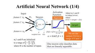
1. 1
Artificial Neural Network (1/4)
…
feature 1 𝑥1
feature 2 𝑥2
feature n 𝑥 𝑛
Input
Neuron
Activation
Function
𝑓 𝑡 = 𝛽 ×
1
1 + 𝑒−𝛼𝑡
𝑤 𝑛
𝑤1
𝑤2
𝑖=1
𝑛
𝑥𝑖 𝑤𝑖 + 𝜃
𝑡
Adjust 𝑤𝑖’s and 𝜃
to reduce 𝑒𝑟𝑟𝑜𝑟,
where
𝑒𝑟𝑟𝑜𝑟 = 𝑡𝑎𝑟𝑔𝑒𝑡 − 𝑓(𝑡)
𝑡𝑎𝑟𝑔𝑒𝑡
𝛼 = 0.667, 𝛽 = 1
𝑤𝑖’s and 𝜃 are initialized
to a range of −
2.4
𝑁
,
2.4
𝑁
,
where 𝑁 is the number of inputs
One neuron only classifies data
that are linearly separable.
We set the
output 𝑓 𝑡 in a
range of 0 and 1
Sigmoid
weighted sum bias

2. 2
Artificial Neural Network (2/4)
feature 1 𝑥1
feature 2 𝑥2
feature 3 𝑥3
feature m 𝑥 𝑚
𝑤𝑖𝑗 𝑝 + 1 = 𝑤𝑖𝑗 𝑝 + 𝛥𝑤𝑖𝑗 𝑝 ,
𝛥𝑤𝑖𝑗 𝑝 = 𝛼𝑥𝑖 𝑝 𝛿𝑗 𝑝 ,
𝛿𝑗 𝑝 = 𝑦𝑗 𝑝 1 − 𝑦𝑗 𝑝 𝑒𝑗(𝑝
𝑒𝑗 𝑝 =
𝑘=1
𝑙
𝛿 𝑘 𝑝 𝑤𝑗𝑘(𝑝
)𝛿 𝑘 𝑝 = 𝑦 𝑘 𝑝 1 − 𝑦 𝑘 𝑝 𝑒 𝑘(𝑝
𝑒 𝑘 𝑝 = 𝑦 𝑑,𝑘 𝑝 − 𝑦 𝑘 𝑝
Error back-propagation
To update 𝑤𝑖𝑗
at iteration 𝑝,
𝑤𝑖𝑗 𝑤𝑗𝑘
𝑥𝑖 𝑦𝑗 𝑦 𝑘
𝛼 is the learning rate,
often set to 0.1~0.5
𝑦1
𝑦2
𝑦3
𝑦𝑙
Input
Layer
Hidden
Layer
Output
Layer
𝑦 𝑑,1
𝑦 𝑑,2
𝑦 𝑑,3
𝑦 𝑑,𝑙
Predicted Actual
…
…
…
…
…
…
…

3. 3
Artificial Neural Network (3/4)
feature 1 𝑥1
feature 2 𝑥2
feature 3 𝑥3
feature m 𝑥 𝑚
𝑤𝑗𝑘 𝑝 + 1 = 𝑤𝑗𝑘 𝑝 + 𝛥𝑤𝑗𝑘 𝑝
)𝛿 𝑘 𝑝 = 𝑦 𝑘 𝑝 1 − 𝑦 𝑘 𝑝 𝑒 𝑘(𝑝
𝑒 𝑘 𝑝 = 𝑦 𝑑,𝑘 𝑝 − 𝑦 𝑘 𝑝
To update 𝑤𝑗𝑘 at iteration 𝑝,
𝑤𝑖𝑗 𝑤𝑗𝑘
𝑥𝑖 𝑦𝑗 𝑦 𝑘
𝑦1
𝑦2
𝑦3
𝑦𝑙
Input
Layer
Hidden
Layer
Output
Layer
𝑦 𝑑,1
𝑦 𝑑,2
𝑦 𝑑,3
𝑦 𝑑,𝑙
Predicted Actual
…
…
…
…
…
…
…
How many iterations required?
𝐸 =
1
2
𝑝=1
𝑁 𝑇
𝑘=1
𝑙
(𝑦 𝑑,𝑘 𝑝 − 𝑦 𝑘(𝑝))2
where 𝐸 is the iteration required, and
𝑁 𝑇 is the number of training samples.

4. 4
Artificial Neural Network (4/4)
Neural
Network
…
…
feature 1
feature 2
feature m
class 1
class 2
class 3
class n
Input Layer
Hidden Layer
Output Layer
Let the output of the activation function
be in a range of 0 and 1
𝑠𝑖𝑔𝑚𝑜𝑖𝑑 𝑥 = 𝛽 ×
1
1 + 𝑒−𝛼𝑥
Sum of the values in
output layer is 1.00

5. 5
𝐼𝑛𝑓𝑜 𝑓𝑛
𝐷 =
𝑗=1
𝑣
𝐷𝑗
𝐷
× 𝐼𝑛𝑓𝑜 𝐷𝑗
𝐼𝑛𝑓𝑜 𝐷 = −
𝑖=1
𝑚
𝑝𝑖 𝑙𝑜𝑔2 𝑝𝑖 ,
𝐼𝑛𝑓𝑜𝑟𝑚𝑎𝑡𝑖𝑛𝐺𝑎𝑖𝑛 𝑓𝑛 = 𝐼𝑛𝑓𝑜 𝐷 − 𝐼𝑛𝑓𝑜 𝑓𝑛
(𝐷
To build a node in the tree, choose a
combination of feature and split value
with the most information gain.
𝑓𝑛 is a chosen feature.
𝐷 is the dataset to be split.
𝐷𝑗 is the 𝑗𝑡ℎ split dataset.
𝑚 is the number of classes
𝑝𝑖 is the percentage of class 𝑖 in
all of the data
≤ 𝑘 𝑡ℎ
𝑠𝑝𝑙𝑖𝑡 𝑣𝑎𝑙𝑢𝑒
> 𝑘 𝑡ℎ
𝑠𝑝𝑙𝑖𝑡 𝑣𝑎𝑙𝑢𝑒
𝑑𝑎𝑡𝑎𝑠𝑒𝑡 𝑜𝑓 𝑚 𝑐𝑙𝑎𝑠𝑠𝑒𝑠
Split into 𝑣 partitions, with 𝑣 − 1 split values.
𝑣 is always 2 for generating a binary tree.
𝑓𝑛
subset
To build a decision tree,
first, calculate the entropy of class in
the dataset.
subset
Decision Tree (1/7)

6. 6
≤ 𝑘 𝑡ℎ
𝑠𝑝𝑙𝑖𝑡 𝑣𝑎𝑙𝑢𝑒
> 𝑘 𝑡ℎ
𝑠𝑝𝑙𝑖𝑡 𝑣𝑎𝑙𝑢𝑒
𝑑𝑎𝑡𝑎𝑠𝑒𝑡 𝑜𝑓 𝑚 𝑐𝑙𝑎𝑠𝑠𝑒𝑠
𝑓𝑛
subsetsubset
Information gain bias towards attributes
with a large number of values
Use GainRatio to overcome the problem
𝑆𝑝𝑙𝑖𝑡𝐼𝑛𝑓𝑜 𝑓 𝑛
𝐷 = −
𝑗=1
𝑣
𝐷𝑗
𝐷
× 𝑙𝑜𝑔2(
𝐷𝑗
𝐷
)
𝐺𝑎𝑖𝑛𝑅𝑎𝑡𝑖𝑜 𝑓𝑛 =
𝐼𝑛𝑓𝑜𝑟𝑚𝑎𝑡𝑖𝑜𝑛𝐺𝑎𝑖𝑛 𝑓𝑛
𝑆𝑝𝑙𝑖𝑡𝐼𝑛𝑓𝑜 𝑓𝑛
𝐷
Decision Tree (2/7)

7. Red Green Blue Cyan Magenta Yellow Achromatic Contrast Saturation Sharpness HarmonicBrightness Class
64.99 19.92 9.25 10.02 5.98 81.39 0.39 67.9 61.01 31.41 57.09 17.23 Good
32.81 7.74 13.88 7.08 11.25 35.6 42.39 37.85 23.87 43.91 53.52 80.97 Bad
90.96 2.56 5.25 11.63 2.4 83.18 0.17 44.93 53.37 34.84 56.08 40.51 Good
13.79 5.4 77.53 4.05 82.54 11.9 0.28 34.91 17.75 44.38 68.3 58.62 Good
81.17 1.94 12.79 21.16 6.3 67.74 1.86 45.63 29.33 19.06 38.86 51.09 Good
55.81 40.33 0.99 0.01 1.21 98.71 0.01 54.35 36.97 41.88 88.76 42.03 Bad
67.49 11.35 17.67 5.36 18.85 73.78 0.68 20.41 31.02 10.47 60.48 59.4 Good
57.01 11.56 2.63 3.54 4.84 65.64 25.25 17.67 23.4 56.72 70.52 93.99 Good
12.89 20.86 62.69 5.18 72.89 19.96 0.12 18.73 28.24 50.94 67.25 75.99 Good
42.34 32.27 17.81 2.61 19.06 73.36 2.15 54.9 31.48 73.59 63.34 53.19 Bad
78.73 3.8 4.4 2.03 6.25 90.78 0.26 47.63 31.74 8.13 74.3 41.43 Good
88.94 0.42 6.57 87.64 0.29 8.7 2.22 45.06 45.37 30.78 55.03 25.35 Good
41.3 0.96 54.24 20.59 47.91 27.33 1.79 33.47 32.16 42.66 48.92 58.08 Good
30.36 29.77 28.48 0.43 46.37 47.34 4.16 25.52 10.42 16.41 62.87 64.71 Good
49.18 1.83 1.83 4.12 0.92 50.38 41.91 52.31 9.73 21.25 72.46 60.26 Good
Red Green Blue Cyan Magenta Yellow Achromatic Contrast Saturation Sharpness HarmonicBrightness Class
11.61 3.07 85 35.65 57.84 2.2 0 81.92 79.27 38.59 74.88 29.51 Bad
16.88 1.78 1.21 7.41 2.12 7.2 78.47 83.21 7.46 19.22 71.61 46.43 Bad
2.48 40.71 1.78 1.75 39.6 0.84 53.84 128.39 24.34 12.5 58.9 23.45 Bad
0 0 0 0 0 0 100 59.11 0 17.03 100 44.58 Bad
Split 1 : If Yellow > 7.2?
Yellow
> 7.2
B
Subtree
Input
< 7.2
7
Decision Tree (3/7)

8. 8
Red Green Blue Cyan Magenta Yellow Achromatic Contrast Saturation Sharpness HarmonicBrightness Class
55.81 40.33 0.99 0.01 1.21 98.71 0.01 54.35 36.97 41.88 88.76 42.03 Bad
42.34 32.27 17.81 2.61 19.06 73.36 2.15 54.9 31.48 73.59 63.34 53.19 Bad
30.36 29.77 28.48 0.43 46.37 47.34 4.16 25.52 10.42 16.41 62.87 64.71 Good
Red Green Blue Cyan Magenta Yellow Achromatic Contrast Saturation Sharpness HarmonicBrightness Class
11.61 3.07 85 35.65 57.84 2.2 0 81.92 79.27 38.59 74.88 29.51 Bad
16.88 1.78 1.21 7.41 2.12 7.2 78.47 83.21 7.46 19.22 71.61 46.43 Bad
2.48 40.71 1.78 1.75 39.6 0.84 53.84 128.39 24.34 12.5 58.9 23.45 Bad
0 0 0 0 0 0 100 59.11 0 17.03 100 44.58 Bad
Red Green Blue Cyan Magenta Yellow Achromatic Contrast Saturation Sharpness HarmonicBrightness Class
64.99 19.92 9.25 10.02 5.98 81.39 0.39 67.9 61.01 31.41 57.09 17.23 Good
32.81 7.74 13.88 7.08 11.25 35.6 42.39 37.85 23.87 43.91 53.52 80.97 Bad
90.96 2.56 5.25 11.63 2.4 83.18 0.17 44.93 53.37 34.84 56.08 40.51 Good
13.79 5.4 77.53 4.05 82.54 11.9 0.28 34.91 17.75 44.38 68.3 58.62 Good
81.17 1.94 12.79 21.16 6.3 67.74 1.86 45.63 29.33 19.06 38.86 51.09 Good
67.49 11.35 17.67 5.36 18.85 73.78 0.68 20.41 31.02 10.47 60.48 59.4 Good
57.01 11.56 2.63 3.54 4.84 65.64 25.25 17.67 23.4 56.72 70.52 93.99 Good
12.89 20.86 62.69 5.18 72.89 19.96 0.12 18.73 28.24 50.94 67.25 75.99 Good
78.73 3.8 4.4 2.03 6.25 90.78 0.26 47.63 31.74 8.13 74.3 41.43 Good
88.94 0.42 6.57 87.64 0.29 8.7 2.22 45.06 45.37 30.78 55.03 25.35 Good
41.3 0.96 54.24 20.59 47.91 27.33 1.79 33.47 32.16 42.66 48.92 58.08 Good
49.18 1.83 1.83 4.12 0.92 50.38 41.91 52.31 9.73 21.25 72.46 60.26 Good
Split 2 : If Green > 29.77?
Yellow
B
Green
Input
> 7.2 > 29.77
≤ 29.77
Subtree
Subtree
≤ 7.2
8
Decision Tree (4/7)

9. 9
Red Green Blue Cyan Magenta Yellow Achromatic Contrast Saturation Sharpness HarmonicBrightness Class
55.81 40.33 0.99 0.01 1.21 98.71 0.01 54.35 36.97 41.88 88.76 42.03 Bad
42.34 32.27 17.81 2.61 19.06 73.36 2.15 54.9 31.48 73.59 63.34 53.19 Bad
Red Green Blue Cyan Magenta Yellow Achromatic Contrast Saturation Sharpness HarmonicBrightness Class
11.61 3.07 85 35.65 57.84 2.2 0 81.92 79.27 38.59 74.88 29.51 Bad
16.88 1.78 1.21 7.41 2.12 7.2 78.47 83.21 7.46 19.22 71.61 46.43 Bad
2.48 40.71 1.78 1.75 39.6 0.84 53.84 128.39 24.34 12.5 58.9 23.45 Bad
0 0 0 0 0 0 100 59.11 0 17.03 100 44.58 Bad
Red Green Blue Cyan Magenta Yellow Achromatic Contrast Saturation Sharpness HarmonicBrightness Class
64.99 19.92 9.25 10.02 5.98 81.39 0.39 67.9 61.01 31.41 57.09 17.23 Good
32.81 7.74 13.88 7.08 11.25 35.6 42.39 37.85 23.87 43.91 53.52 80.97 Bad
90.96 2.56 5.25 11.63 2.4 83.18 0.17 44.93 53.37 34.84 56.08 40.51 Good
13.79 5.4 77.53 4.05 82.54 11.9 0.28 34.91 17.75 44.38 68.3 58.62 Good
81.17 1.94 12.79 21.16 6.3 67.74 1.86 45.63 29.33 19.06 38.86 51.09 Good
67.49 11.35 17.67 5.36 18.85 73.78 0.68 20.41 31.02 10.47 60.48 59.4 Good
57.01 11.56 2.63 3.54 4.84 65.64 25.25 17.67 23.4 56.72 70.52 93.99 Good
12.89 20.86 62.69 5.18 72.89 19.96 0.12 18.73 28.24 50.94 67.25 75.99 Good
78.73 3.8 4.4 2.03 6.25 90.78 0.26 47.63 31.74 8.13 74.3 41.43 Good
88.94 0.42 6.57 87.64 0.29 8.7 2.22 45.06 45.37 30.78 55.03 25.35 Good
41.3 0.96 54.24 20.59 47.91 27.33 1.79 33.47 32.16 42.66 48.92 58.08 Good
49.18 1.83 1.83 4.12 0.92 50.38 41.91 52.31 9.73 21.25 72.46 60.26 Good
Red Green Blue Cyan Magenta Yellow Achromatic Contrast Saturation Sharpness HarmonicBrightness Class
30.36 29.77 28.48 0.43 46.37 47.34 4.16 25.52 10.42 16.41 62.87 64.71 Good
Split 3 : If Red > 30.36?
Yellow
B
Green
Input
> 7.2
≤ 7.2
> 29.77
≤ 29.77
Subtree
Red
G
B
> 29.77
≤ 29.77
9
Decision Tree (5/7)

10. 10
Red Green Blue Cyan Magenta Yellow Achromatic Contrast Saturation Sharpness HarmonicBrightness Class
55.81 40.33 0.99 0.01 1.21 98.71 0.01 54.35 36.97 41.88 88.76 42.03 Bad
42.34 32.27 17.81 2.61 19.06 73.36 2.15 54.9 31.48 73.59 63.34 53.19 Bad
Red Green Blue Cyan Magenta Yellow Achromatic Contrast Saturation Sharpness HarmonicBrightness Class
11.61 3.07 85 35.65 57.84 2.2 0 81.92 79.27 38.59 74.88 29.51 Bad
16.88 1.78 1.21 7.41 2.12 7.2 78.47 83.21 7.46 19.22 71.61 46.43 Bad
2.48 40.71 1.78 1.75 39.6 0.84 53.84 128.39 24.34 12.5 58.9 23.45 Bad
0 0 0 0 0 0 100 59.11 0 17.03 100 44.58 Bad
Red Green Blue Cyan Magenta Yellow Achromatic Contrast Saturation Sharpness HarmonicBrightness Class
30.36 29.77 28.48 0.43 46.37 47.34 4.16 25.52 10.42 16.41 62.87 64.71 Good
Yellow
B
Green
Input
> 7.2
≤ 7.2
> 29.77
≤ 29.77
Achromatic
Red
G
B
> 29.77
≤ 29.77
≥ 41.91
B
G
Split 4 : If Achromatic <41.91?
Red Green Blue Cyan Magenta Yellow Achromatic Contrast Saturation Sharpness Harmonic Brightness Class
64.99 19.92 9.25 10.02 5.98 81.39 0.39 67.9 61.01 31.41 57.09 17.23 Good
90.96 2.56 5.25 11.63 2.4 83.18 0.17 44.93 53.37 34.84 56.08 40.51 Good
13.79 5.4 77.53 4.05 82.54 11.9 0.28 34.91 17.75 44.38 68.3 58.62 Good
81.17 1.94 12.79 21.16 6.3 67.74 1.86 45.63 29.33 19.06 38.86 51.09 Good
67.49 11.35 17.67 5.36 18.85 73.78 0.68 20.41 31.02 10.47 60.48 59.4 Good
57.01 11.56 2.63 3.54 4.84 65.64 25.25 17.67 23.4 56.72 70.52 93.99 Good
12.89 20.86 62.69 5.18 72.89 19.96 0.12 18.73 28.24 50.94 67.25 75.99 Good
78.73 3.8 4.4 2.03 6.25 90.78 0.26 47.63 31.74 8.13 74.3 41.43 Good
88.94 0.42 6.57 87.64 0.29 8.7 2.22 45.06 45.37 30.78 55.03 25.35 Good
41.3 0.96 54.24 20.59 47.91 27.33 1.79 33.47 32.16 42.66 48.92 58.08 Good
49.18 1.83 1.83 4.12 0.92 50.38 41.91 52.31 9.73 21.25 72.46 60.26 Good
Red Green Blue Cyan Magenta Yellow Achromatic Contrast Saturation Sharpness Harmonic Brightness Class
32.81 7.74 13.88 7.08 11.25 35.6 42.39 37.85 23.87 43.91 53.52 80.97 Bad
10
Decision Tree
(6/7)

11. Decision Tree (7/7) - Pruning
• A problem for decision tree is overfitting
• Pruning helps the tree classify unseen data more accurately
• We apply post-pruning to solve the overfitting problem
• For compare the accuracy of class prediction before and after pruning each
sub-tree
• If the accuracy is higher after pruning, accept the pruning
• Otherwise, keep the original sub-tree
Before pruning After pruning
(Replacing the sub-tree with a class leaf)

12. 12
Decision Tree
class
●, 𝑥 + 0.5 ≤ 𝑦
●, 𝑥 + 0.5 > 𝑦
Easily classified by
linear regression
But decision tree is
axis-aligned!
Input sample data
with two classes
We want to separate
the data efficiently

13. 13
Decision Tree
Principal
Component
Analysis
(PCA)
1st component
2nd component
Input data
(not axis-aligned)
Axis-aligned
(Linear transformations)
Principal Component Analysis (PCA) is often
used for dimension reduction, but is also
helpful for improving the performance of
decision tree.