heducation puspouse

1. An algorithm is a sequence of instructions followed to solve a problem.
A parallel algorithm is an algorithm that can execute several instructions simultaneously on
different processing devices and then combine all the individual outputs to produce the final
result.
The function of concurrent processing that can divide a complex task and process it multiple
systems to produce the output in quick time.
Concurrent processing is essential where the task involves processing a huge bulk of complex
data. Examples include − accessing large databases, aircraft testing, astronomical calculations,
atomic and nuclear physics, biomedical analysis, economic planning, image processing, robotics,
weather forecasting, web-based services, etc.
Model of Computation
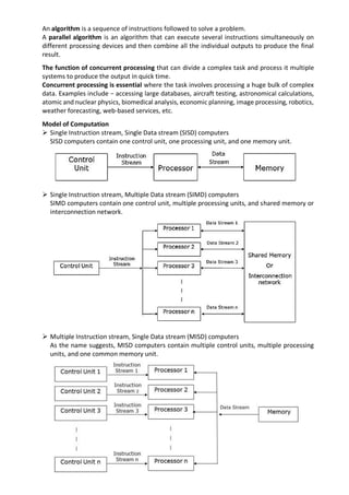
➢ Single Instruction stream, Single Data stream (SISD) computers
SISD computers contain one control unit, one processing unit, and one memory unit.
➢ Single Instruction stream, Multiple Data stream (SIMD) computers
SIMD computers contain one control unit, multiple processing units, and shared memory or
interconnection network.
➢ Multiple Instruction stream, Single Data stream (MISD) computers
As the name suggests, MISD computers contain multiple control units, multiple processing
units, and one common memory unit.

2. ➢ Multiple Instruction stream, Multiple Data stream (MIMD) computers
MIMD computers have multiple control units, multiple processing units, and a shared
memory or interconnection network.
Parallel Algorithm Models –
1. Data parallel model
- tasks are assigned to processes.
- consequence of single operations.
- being applied on multiple data items.
- disadvantage - increases with the size.
2. Task Graph Model
- quantity of data associated with the tasks.
- improve the cost of data movement.
- problems are divided into atomic tasks and implemented as a graph.

3. 3. Work Pool Model
- dynamically assigned to balancing load.
- used when the quantity of data associated with tasks is comparatively smaller than the
computation associated with the tasks.
- assigning of tasks is centralized.
4. Master-Slave Model
- one or more master processes generate task and allocate it to slave processes. Maybe
allocated it.
- master can estimate the volume of the tasks.
- a random assigning can do a satisfactory job of balancing load.
- slaves are assigned smaller pieces of task at different times.
5. Pipeline Model
- set of data is passed on through a series of processes, each of which performs some tasks
on it.
- arrival of new data generates the execution of a new task.
- chain of producers and consumers.
- process in the queue.

4. 6. Hybrid Models
- multiple models applied hierarchically
Example − Parallel quick sort
Time complexity is a measure of the amount of time required by an algorithm to run as a
function of the size of its input. It estimates the growth rate of the algorithm's running time
relative to the input size. In other words, time complexity provides an understanding of how
the algorithm's performance scales with the size of the problem.
Classify Time complexity
Worst-case complexity − When the amount of time required by an algorithm for a given
input is maximum.
Average-case complexity − When the amount of time required by an algorithm for a given
input is average.
Best-case complexity − When the amount of time required by an algorithm for a given input
is minimum.
Asymptotic notation is the easiest way to describe the fastest and slowest possible
execution time for an algorithm using high bounds and low bounds on speed. For this, we
use the asymptotic notation in Parallel algorithm.
Big O notation
In mathematics, Big O notation is used to represent the asymptotic characteristics of
functions. The function − f(n) = O(g(n))
If there exists positive constants c and n such that f(n) ≤ c * g(n) for all n where n ≥ n .
Omega notation
Omega notation is a method of representing the lower bound of an algorithm’s execution
time. The function − f(n) = Ω (g(n))
If there exists positive constants c and n such that f(n) ≥ c * g(n) for all n where n ≥ n .
Theta Notation
Theta notation is a method of representing both the lower bound and the upper bound of
an algorithm’s execution time. The function − f(n) = θ(g(n))
If there exists positive constants c ,c , and n such that c1 * g(n) ≤ f(n) ≤ c2 * g(n) for all n
where n ≥ n .