Advanced statistical approach to customer risk rating

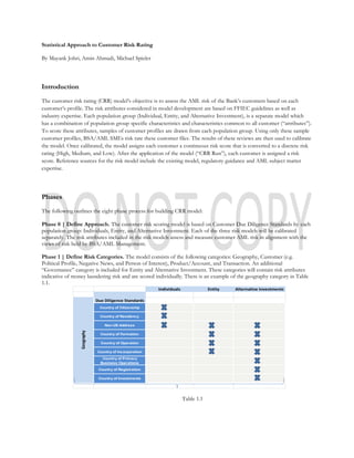
1. Statistical Approach to Customer Risk Rating
By Mayank Johri, Amin Ahmadi, Michael Spieler
Introduction
The customer risk rating (CRR) model’s objective is to assess the AML risk of the Bank’s customers based on each
customer’s profile. The risk attributes considered in model development are based on FFIEC guidelines as well as
industry expertise. Each population group (Individual, Entity, and Alternative Investment), is a separate model which
has a combination of population group specific characteristics and characteristics common to all customer (“attributes”).
To score these attributes, samples of customer profiles are drawn from each population group. Using only these sample
customer profiles, BSA/AML SMEs risk rate these customer files. The results of these reviews are then used to calibrate
the model. Once calibrated, the model assigns each customer a continuous risk score that is converted to a discrete risk
rating (High, Medium, and Low). After the application of the model (“CRR Run”), each customer is assigned a risk
score. Reference sources for the risk model include the existing model, regulatory guidance and AML subject matter
expertise.
Phases
The following outlines the eight phase process for building CRR model:
Phase 0 | Define Approach. The customer risk scoring model is based on Customer Due Diligence Standards by each
population group: Individuals, Entity, and Alternative Investment. Each of the three risk models will be calibrated
separately. The risk attributes included in the risk models assess and measure customer AML risk in alignment with the
views of risk held by BSA/AML Management.
Phase 1 | Define Risk Categories. The model consists of the following categories: Geography, Customer (e.g.
Political Profile, Negative News, and Person of Interest), Product/Account, and Transaction. An additional
“Governance” category is included for Entity and Alternative Investment. These categories will contain risk attributes
indicative of money laundering risk and are scored individually. There is an example of the geography category in Table
1.1.
Table 1.1
Individuals Entity Alternative Investments
Country of Citizenship
Country of Residency
Non-US Address
Country of Formation
Country of Operation
Country of Incorporation
Country of Primary
Business Operations
Country of Registration
Country of Investments
Geography
Due Diligence Standards

2. Phase 2 |Data Analysis. Determine the relevant risk attributes for each risk categories, by first conducting working
group sessions to conceptually agree on the risk attributes, then using existing customer data for the following:
 Assessing data completeness (% of non-null/blank values)
 Assessing variation within a given variable
Risk attributes that have low data completeness or low variation are removed. Low data completeness means a large
portion of the customers don’t have usable values, making it a meaningless attribute for the majority of customers. Low
variation means a large portion of the customers have the same value, complicating the model with additional attributes
that don’t help differentiate any one customer from the rest.
Phase 3 |Correlation Test. To give a preliminary understanding of the levels pairwise correlation between attributes,
test using various correlation coefficients based on the data types (e.g. binary, ordinal and continuous). Appropriate
pairwise correlation coefficients are as follows:
i. Binary - Binary: phi coefficient (mean square contingency coefficient)
ii. Binary - Continuous: ANOVA to evaluate how likely the correlation between two
variables is by chance
iii. Ordinal - Continuous: Kendall’s(τ)
iv. Ordinal – Ordinal: Spearman’s (rs)
A correlation study would entail quantifying the relationships among all the attributes (as opposed to pairwise) to
evaluate the relationship between one attribute relative to all of the others. This study can be directly used to decide
which attributes need to stay in the model, and whether their contribution is at the additive level or also needs to be
accounted at two-way (or three-way) interactive level (s). Highly pairwise correlated (> 90%) attributes suggest that one
might be eliminated without losing the accuracy of the model, but not if high multicollinearity, which can only be
quantified at the model level, also exists. Below is the interpretation of the correlation study.
 Highly pairwise correlated (> 90%) attributes: leave only one in the model. In order to
decide which one to remove one can calculate “coefficient of partial determination” and
eliminate the one with lower value
 Attributes with no or low (<5%) correlation: leave both in the model; there is strong
evidence that including the interaction term of these two attributes would not significantly
contribute to the accuracy of the model
 Attributes with some level of correlation: leave both in the model; interaction term should
be investigated at the model level analysis
Phase 3 |Sampling. For each population group, draw samples to cover all combinations of risks for SME risk rating.
The outcome of the SME risk rating is the labeled data (label being the ranking of the customer) which is used to “learn”
the regression model. The samples may be generated as follows:
 Organize data into a list with each row representing a specific combination and the last
column showing the frequency of the case
 Select the target sample size: n
 For each row, develop the binomial marginal distribution
 Determine expected value of each cell based on the selected sample size

3.  For rare event cases, augment to have size of at least N= 10k/p where k is the number of
covariates and p is the probability of the rare event case
Phase 4 |SME Rating. Reviewing one sampled (from phase 3) customer at a time, an AML SME looks at that
customer’s values for each risk attribute and ascertains a risk rating or high, medium, or low, based regulatory guidance
and the BSA/AML department’s risk tolerance.
Phase 5 |Model Calibration. Conduct statistical analysis using SME’s risk rating to calibrate the model. Model
calibration has the following steps:
The risk rating of samples, as labeled by SME, is fitted by ordinal logistic regression. The developed model is used to risk
rate the entire population. Ordinal logistic model assigns each customer, based on the customer’s attributes, to a
distribution interval (i.e., risk tier). Fig. 1.2 (typical result of ordinal logistic regression) shows a schematic representation
of the model result.
Figure 1.2
Phase 6 |Model Performance Evaluation. Given the structure of CRR data, a logistic regression is used to relate
selected attributes to customer risk ranks (as determined by an SME). An optimized model is developed based on the
performance of the selected attributes (i.e., how much does the attribute contribute toward the accuracy of the model?)
and how well the optimized model performs vis-à-vis the benchmark model.
 A Wald test is used to decide if an attribute needs to be included in the optimized model by
quantifying how far the estimated parameter is from zero. The Wald test can also be used for
multiple parameters simultaneously
 A log-likelihood ratio test is used to compare “reduced” (candidate optimized) models with
the benchmark model. The benchmark model, which includes all the attributes and their
second or/and higher level interaction terms, is also the most restrictive model. This means
that the benchmark model has the best performance within the current data, but has
diminished generalization capability. In general one tries to select the most simplified model
which still has acceptable performance
 McFadden pseudo-R2 is used to gauge how much the logistic regression model explains a
variation in the response. This is considered a similar measure to the ubiquitous R2 used in
linear regression. The value of pseudo- R2 ranges between 0 and 1; values close to 0 indicates
the model has no predictive capability

4.  Uncertainty of the final model is quantified to evaluate how well the model would apply to
future customers. The uncertainty may be characterized at two levels:
i. Uncertainty of the selected attributes represented by the variance of the regression
coefficients
ii. Residual uncertainty represented by the standard error of the model
Assess if the differences between model prediction and SME ratings are within acceptable model error rate. Confirm the
model output’s alignment with working group’s views and expectations. If it is not, go back to phase 5 and calibrate the
model again.
Phase 7 |Model Implementation. Once the evaluation is complete and the result is satisfactory, the model is
implemented and run on a regular schedule in an automated fashion. The outcome of the model can potentially drive
various processes, including periodic due diligence reviews and stratified transaction monitoring thresholds.