SlideShare a Scribd company logo
1 of 49
Review Parameters: Model Building & Interpretation and Model
Tuning
1. Model Building
a. Assessments and Rationale of Various Models Employed to
Predict Loan Defaults
The z-score formula model was employed by Altman (1968)
while envisaging bankruptcy. The model was utilized to forecast
the likelihood that an organization may fall into bankruptcy in a
period of two years. In addition, the Z-score model was
instrumental in predicting corporate defaults. The model makes
use of various organizational income and balance sheet data to
weigh the financial soundness of a firm. The Z-score involves a
Linear combination of five general financial ratios which are
assessed through coefficients. The author employed the
statistical technique of discriminant examination of data set
sourced from publically listed manufacturers. A research study
by Alexander (2012) made use of symmetric binary alternative
models, otherwise referred to as conditional probability models.
The study sought to establish the asymmetric binary options
models subject to the extreme value theory in better explicating
bankruptcy.
In their research study on the likelihood of default models
examining Russian banks, Anatoly et al. (2014) made use of
binary alternative models in predicting the likelihood of default.
The study established that preface specialist clustering or
mechanical clustering enhances the prediction capacity of the
models. Rajan et al. (2010) accentuated the statistical default
models as well as inducements. They postulated that purely
numerical models disregard the concept that an alteration in the
inducements of agents who produce the data may alter the very
nature of data. The study attempted to appraise statistical
models that unpretentiously pool resources on historical figures
devoid of modeling the behavior of driving forces that generates
these data. Goodhart (2011) sought to assess the likelihood of
small businesses to default on loans. Making use of data on
business loan assortment, the study established the particular
lender, loan, and borrower characteristics as well as
modifications in the economic environments that lead to a rise
in the probability of default. The results of the study form the
basis for the scoring model. Focusing on modeling default
possibility, Singhee & Rutenbar (2010) found the risk as the
uncertainty revolving around an enterprise’s capacity to service
its obligations and debts.
Using the logistic model to forecast the probability of bank loan
defaults, Adam et al. (2012) employed a data set with
demographic information on borrowers. The authors attempted
to establish the risk factors linked to borrowers are attributable
to default. The identified risk factors included marital status,
gender, occupation, age, and loan duration. Cababrese (2012)
employed three accepted data mining algorithms, naïve
Bayesian classifiers, artificial neural network decision trees
coupled with a logical regression model to formulate a
prediction model that employs a large data set. The study
concluded that naïve Bayesian classifiers proved to be superior
with an accuracy of prediction standing at 92.4 percent.
Focusing on the models of loan defaults in the case of SMEs as
rare action, Rafaella (n.d.) employed comprehensive acute
values degeneration. The study inferred that the logistic models
had some downsides such as underestimation of the likelihood
of loan default. Using binary GEV model to foresee the
probability of loan default and established to perform better as
compared to the logical regression model.
b. Model Building Problem and Variable Selection
An analyst is invariably faced with a wide spectrum of possible
prospective regressors when dealing with practical problems. Of
all these regressors only a small number are likely to be
significant. Determining the suitable division of regressors for
the model is referred to as the variable selection problem.
Normally, there are two conflicting goals involved in
formulating a regression model that encapsulates a subset of the
obtainable regressors. On one hand, the analysis necessitates the
model to contain as many regressors as feasible in an effort to
ensure that the data content in these aspects can influence the
predicted value (y). On the other hand, the model is expected to
encapsulate as a small number of regressors as possible since
the variance of the prediction rises as the number of regressors
enlarges.
Rubbing out variables potentially brings about prejudice into
the estimations of the coefficient of the maintained variables as
well as the retorts. Model over-fitting, which implies to
inclusion of variables with entirely zero regression coefficients
in the data population in the model, does not establish prejudice
when estimating population regression coefficient, in the event
that the usual regression assumptions are adhered to.
Nonetheless, there is need to ascertain that over-fitting does not
bring about adverse co-linearity.
Variable selection process involves the following fundamental
steps:
i. Indicating the maximum model in consideration
ii. Outlining the selection model criterion
iii. Specifying the strategy for variables selection
iv. Carrying out the indicated evaluation
v. Assessing the chosen model validity
I. Indicating the Maximum Model
The maximum model is considered to be the biggest model,
implying one with the largest number of predictor variables, and
is considered at every juncture of model selection process. The
choice of the maximum model has particular constraints
imposed on it ensuing from the certain data sample to be
assessed. The most fundamental constriction is the fact that
degrees of freedom errors ought to be positive. Consequently,
or unvaryingly, with being the number of observation while
represents the number of predictors, resulting to coefficient of
regression inclusive of the intercept. Generally, it is plausible
to obtain a large freedom of error degrees. This implies that as
the sample size becomes smaller, the maximum model gets
smaller. The biggest challenge is then is establishing the
number of degrees of freedom that are required. The feeblest
prerequisite is . An agreed thumb rule for regression is having
not less that 5 or 10 observations for each predictor. In this
case,
II. Criteria for Assessment of Subset Regression Models
There is availability of various criteria that can be employed in
the assessment of the subset regression models. The utilized
criterion is dependent on the intention of the model. Letting
and represent the sum of squares regression and sum of squares
residuals, correspondingly, for a model with terms, which
implies regressors as well as as intercept term:
a. F-Test Statistic
This represents another practical principle for outlining the best
model that is employed to compare the reduced and full models.
The F- Test statistic is obtained as below:
It is possible to compare this statistic to an F- distribution using
as well as freedom degrees. In the event that Fp is not
significant, smaller variables model is used.
b. Coefficient of Determination
This is the quantity of the sufficiency of the regression model
that has largely been utilized. Letting represent the coefficient
of determination for model subset of terms, then
amplifies as increases and obtains a maximum value when .
Subsequently, one employs this criterion through addition of
regressors to the model up until there is an further variable
generates a small increase in .
If we consider in that and the value of for the full mode is ,
any regressors variables subset that generates an larger than is
referred to as the - adequate () subset. This implies that is not
considerably dissimilar from the .
c. Mallow’s Cp Statistic
This approach is another candidate for selection criterion that
involves Mallow’s. In this case
The criterion aids in establishing the various variables that
need to be included in the best model, following the fact that it
attains a value just about if is approximately equivalent to .
d. PRESS
An analyst can choose the subset regression model subject to a
diminutive value of PRESS. Although PRESS has perceptive
application, certainly for the forecast problem, it is not an easy
function of the sum of squares residual, and formulating an
algorithm for variable selection on the basis of this criterion is
not clear-cut. This statistic, is nonetheless, potentially
instrumental, in discriminating between models.
e. Logic Regression Model
This model is invariable employed to categorical variables in
the model that assume only two probable outcomes implying
success or failure. The logistic regression assumes the following
form:
Computing the antilog of the above equation, an equation that
can be utilized in the probability of the occurrence of an event
is derived as follows:
represents the likelihood of the outcome desired or event. This
model will be instrumental in forecasting the probability of loan
default.
f. Lineal Regression Model
This model makes use of a statistical approach where the
desired value is represented as a linear combination of sets of
explanatory variables. In the event that the linear regression
makes use of one independent variable, it is referred to as a
simple linear regression. Denotation for a linear regression is as
shown below:
Where
= Dependent variable
= intercept parameter
= Coefficient of regression (slope parameter)
= Error term
= Independent variable
III. Specifying The Strategy For Variables Selection
a. Possible Regression Procedure
This procedure calls for fitting of every possible equation of
regression connected to each probable amalgamation of the
independent variables. Assuming to be the intercept term and it
is included in all equations, then the number of prospective
regressors is , and the total equations to be computed and
evaluated are . Consequently the number of equations to be
evaluated rises swiftly with an augment in the number of
prospective regressors.
b. Backward Elimination Procedure
This procedure starts with a model that encapsulates all the
prospective regressors. Accordingly, the F-statistic is calculated
for every regressor as if it were the final variable to be added to
the model. The minimum partial F-statistics is evaluated against
the pre-selected value (FOUT). As a way of illustration, if the
minimum value of partial F does not exceed the FOUT, the
regressor is eliminated from the model. At this point, a model
with regressors is fit, and the new partial F-statistic for the
resultant model is computed. The procedure is repeated until the
smallest F value is greater or equal to the pre-selected cutoff
value (FOUT).
c. Forward Selection Procedure
This process starts with assuming that there are no regressors in
the model except for the cut-off. An attempt is made to
determine the best possible subset through insertion into the
model one at a time. At every stage, the regressor that largely
partially correlates with, or the correspondingly highest F-
statistic provided the other regressors in the model, is added to
the model in the event its partial F- statistic is larger than the
pre-selected starting point FIN.
d. Stepwise Regression Procedure
This regression procedure is an adapted version of the forward
regression that allows the reevaluation, at every stage, of the
variables integrated in the model in the preceding steps. A
variable previously entered in the model may end up being
redundant at higher steps due to its connection with other
variables consequently incorporated to the model.
2. Model Performance Evaluation
Regression models, on one hand, involve prediction of incessant
values through observing from a number of independent
variables. Classification, otherwise known as regression
pipeline involves three basic steps. First, the initial
configuration of the model is carried out and the output is
predicted subject to certain input. Second, the predicted value is
evaluated against a target value as well as the model
performance quantity computed. Third, there is iterative fine-
tuning of the many model variables in an effort to obtain the
most favorable value of the performance metric. To attain the
optimal value of the standard involves different efforts and
tasks for different constant performance standard. Regression
deals with prediction of the aspect of the outcome variable at a
certain time aided by other correlated independent variables.
Unlike the classification action, the prediction task obtains
outputs that are continuous in value within a specified range.
a. Prediction
Prediction model types deal with ratio or interval dependent
variables, while classification types of models involve
categorical, either ordinal or nominal, dependent variables. For
loan defaults prediction models, the ratio dependent variables
include: customer’s revenue, acquisition cost of customers,
return on investment, and response time. Prediction models
make use of regression, neural networks, and decision trees
methods. Outline below are some of the evaluation methods for
prediction models.
i. MAE/ MAD
MAE or MAD refers to mean absolute error or deviation which
is obtained through the following expression:
ii. Average Error
This value is comparable to MAD apart from the fact that it
keeps the error sign, such that positive errors cancel out with
negative errors of similar magnitude. Average error provides an
indication if the predictions obtained are under-predicting,
average, or over-predicting the desired response. The Average
error is obtained as follows:
iii. MAPE
MAPE stands for Mean Absolute Percentage Error and
represents the measure that provides the score of how
predictions deviate from the actual values in percentage.
iv. RMSE
The root-mean-squared error (RMSE) is similar to the standard
error of prediction, apart from it is calculated on the validation
data as opposed to the training data. It attains the same units as
the predicted variable.
v. Total SSE
Total SSE is the total sum of the squared errors.
vi. Area Under the ROC Curve (AUC- ROC)
One of the popular metrics used in industries is the ROC curve
having the biggest advantage that it is independent of the
change in proportion of responders. Therefore, for each
sensitivity there is a different specificity with the two varying
as shown:
The plot between sensitivity and (1-specifity) indicates the ROC
curve. (1-specificity) is referred to as false positive rate as well
while sensitivity is also referred to as True Positive rate. For
the current case the ROC curve is as follows:
A single point in the ROC plot will indicate a model which
gives class as output. Since judgment needs to be taken on a
single metric and not using multiple metrics, such models
cannot be compared with each other. A model with parameters
(0.2, 0.8) and a model with parameter (0.8, 0.2) can be resulting
from the same model for instance hence these metrics should
not be compared directly.
We were lucky in the case of probabilistic model to get a single
number which was AUC-ROC. However a look at the whole is
needed to make a conclusive decision. It is also possible for one
model to perform better in one region and another better in
other. Of the response rate, the ROC curve is almost
independent on the other hand since it has two axes originating
from columnar calculations of confusion matrix. For both x and
y axis, the numerator and denominator will change on similar
scale of response rate shift.
b. Classification
i. Confusion Matrix
A confusion matrix refers to a square matrix of NxN nature,
where N represents the number of outcomes being predicted.
For a confusion matrix, accuracy is considered as the fraction of
the total predictions number that is accurate. Precision, also
referred to as Positive Predictive Value, represents the
percentage of the positive predictions that were identified
accurately. On the other hand, Negative Predictive Value is
considered to be the proportion of cases identified correctly that
are negative. Specificity is taken to be the fraction of the actual
negative outcomes that have been identified correctly. Below is
an illustration of a Confusion Matrix:
Confusion Matrix
Target
Model
Positive
a
b
Positive Predictive Value
a/(a+b)
Negative
c
d
Negative Predictive Value
d/(c+d)
Sensitivity
Specificity
Accuracy = (a+d)/(a+b+c+d)
a/(a+c)
d/(b+d)
ii. Sensitivity
Ensuing from confusion matrix, sensitivity is obtained through
the expression below
iii. Specificity
Also computed from the confusion matrix, the expression for
specificity is as show:
3. Best Model Interpretation
Bank loan defaults are a rare occurrence but when such
occurrence takes place it may result in incurring of loss. The
daily operations of the banks can be affected by such extreme
occurrences thus leading to adverse impacts on a country’s
economy. Statisticians and analysts have invariably focused on
this concern which has led to proposal of various models in
addressing the problem. Some of the popular models with load
defaults include standard discriminant model, the Z-score, and
logistic regression models. This study prefers the use of
logistic regression model in the assessment of bank loans
defaults. Logistic regression model has been instrumental in
credit risk evaluations in the financial setting. The primary
benefit of logistic regression model is attributable to the fact
that it is easily understood, easy implementation, and superior
performance (Gilli & KeIlezi, 2000). Additionally, the model
outmaneuvers linear regression due to the fact that it mitigates
multiple concerns. For instance, linear regression attains a
regression output that is negative or with a value greater than 1,
which is impossible to obtain likelihood (Goodhart, 2011).
Linear regression deals with this issue through provision of an
incessant spectrum of values between 0 and 1 that maintaining
the regression output to values between 0 and 1.
Previous studies have proposed models for the prediction of
loan defaults through the use of two dissimilar classifiers which
are Cox proportional hazard algorithm and logistic regression in
an effort to predict customers who are likely to default on bank
loans. This study relies on logistic regression coupled with
random forest classifier in predicting likelihood of load
defaulting.
a. Logistic Regression Model
Logistic regression (LR) model is a predictive technique that is
largely employed in forecast and classification phenomena. In
this model the desired variable is a non-linear function of
likelihood of being positive (Thomas, 2000). In addition, the
results of LR classification are sensitive to correlations that fall
between the independent variables. Subsequently, the variables
inserted in formulating the model ought not be sturdily
correlated. It is assumed that the non-linearity of credit data
diminishes the accuracy of the LR accuracy. It follows
therefore; the primary goal of the LR model of credit scoring is
to establish the conditional likelihood of every application
innate in a particular category (Yap et al., 2011). Customers
who are likely to default or those who are not likely to default
on loan are assessed subject to the values of the descriptive
variables of the loan application.
It is vital for every loan application to be allotted only one
category of dependent variable. Nonetheless, the LR model
restricts the attainment of the forecast values of dependent
outcome variable to occur in the range between 0 and 1.
Logistic regression is a popular technique of modeling that
categorizes the loan applicants into two classes, through the use
of a set of predictive variables (Akkoc, 2012). The following
expression is the general representation of LR model.
-representing the likelihood of a customer being “good” with
being the function of predictive variables (: age, : loan amount,
: loan amount, and : professional class) indicating the
characteristics of the loan applicant.
is the intercept, with = (1,….,4) indicating the coefficients
linked to the respective ( = 1,…, 4).
stands for the default occurrence ()
is the term for errors.
It is pertinent to note that multi-colinearity is an unfavorable
aspect of the logistic regression model. However, it is not a
substantial concern since the credit scoring model for loans is
formulated for purposes of prediction.
b. Discriminant Analysis (DA)
The discriminant analysis is aims at finding the discriminant
function and to classify items into one of two or more groups
having certain features describing those items. To maximize the
difference between two groups is the main purpose of the
discriminant analysis, while the differences among particular
members of the same group are minimized. One group consists
of good borrowers (non-defaulters - group A) and the other the
bad ones (already-defaulters – group B) in the sphere of credit
risks models. By means of the discriminant variable – score Z
the differences are measured. For a given borrower I, the score
is calculated as follows:
Where x represents a given character, y stands for the
coefficient within the estimated model and n denotes a number
of indicators.
A linear combination of the independent variables is what the
DA seeks to find. The purpose been to classify the observations
into equally exclusive groups as precisely as possible. This is
achieved by maximizing the variance of the two ratio of among-
groups to within groups. The discriminant function bears the
following form:
Where denotes the jth independent variable, represents the jth
independent variable and Z shows the discriminant score that
that maximizes the difference between the two.
In this study, four variables which are considered as the
discriminant variables were used. In the chosen sample, they
were applied to find out the fitted discriminant score which will
signify the discriminant criterion allowing distinguishing
between the default and the non-default borrowers.
c. Significance of the Model and Interpretation of the
Coefficients
Logistic regression is only practical for large samples; this
makes the checking of lacks of multi-collinearity among
variables/items essential. Due to the reduced number of
explanatory variables in our study, however this issue isn’t
raised. Before interpreting estimate coefficients, we can ask
ourselves of the quality or the general implication of the model
by adopting the R-square of Cox and Snell, which is can be
determined by use of the following formula:
The R-square stands for the explained variance of the
model. We find that the R-square of the Cox and Snell is
equivalent to 0.9592, indicating a right fitted model.
The table below presents the model summary.
Model Summary
Comparison criteria
Values
Deviance (dev)
44.49
Degree of freedom (df)
599
Chi-square test
661.236
Dispersion
0.39
From the table it is evident that the Chi-square value is higher
than the deviance (dev) this makes the model globally
significant.
d. Analysis of Sensitivity and Predictive Power of Model
The model in testing shows a specificity of 1.526% and a
sensitivity of 99.41%. The misclassification rate of the default
payment in the category of the non-defaults is represented of
0.586%. This proves the successful prediction of the quality of
borrowers by the model. From the finding s the model
categorizes 89% of the annotations of our sample. In terms of
the capacity of prediction, could be stronger, but we are to put
in mind the trial nature of this model.
The following table serves as an illustration that indicates the
model prediction power along with the analysis of sensitivity.
No. of Observed Borrowers
Total
Default Likelihood > 0.5 (y=1)
Non-Default Likelihood < 0.5 (y=0)
Default
364
4
368
Default prob. < 0.5 (y=1)
Non-default prob. > 0.5 (y=0)
Non-default
2
236
265
Total
366
267
633
4. Model Tuning and Validation
a. Relevance Weighed Ensemble Model for Anomaly Detection
Detection of anomaly is instrumental in online-data mining
processes. The main concern associated with detection of
incongruity is the dynamically evolving nature of the various
monitoring settings. This results in a challenge for conventional
anomaly detection techniques in data streams, which take up a
relatively static monitoring setting. In a setting that is
intermittently altering, referred to as the switching data streams,
static techniques result into large rate of error through false
positives (Yang et al., 2009). There need to take on a system
that can identify from the history of typical actions in streams
of data, to deal with the vibrant environments. This occurs
while taking into account the aspect that not all periods of time
in the past are significantly pertinent (Aggarwal, 2012).
Subsequently, a relevance-weighed ensemble model is projected
for identifying the typical actions revolving around credit rating
and it forms the foundation for incongruity detection technique.
This approach is instrumental in enhancing the uncovering
accuracy through employment of relevant history, while
maintaining computational efficiency. The relevance-weighed
ensemble model offers a pertinent contribution by utilization of
ensemble approaches for detecting anomaly in data steams used.
It is possible to achieve considerable enhancements through
artificial and real data steams as compared to other modern
detection algorithms of abnormality for streams of data.
b. Model Tuning
Most regression as well as classification models are largely
adjustable in that they have the capacity to model complex
relationships. There are tuning parameters that administer
adaptability of every model, ensuring that every model can
pinpoint predictive behaviors as well as frameworks within the
data. Nonetheless, these tuning attributes can establish
predictive outlines that are not reproducible. This aspect is
referred to as over-fitting. Over-fit models normally have
superior predictivity for the data samples on which they are
generated from, but show low predictivity for fresh samples
(Steyerberg, 2010).
Most of models have significant attributes that cannot be
unswervingly predicted from the data. For instance, in the K-
nearest neighbor categorization model, a fresh sample is
estimated subject to the K-closest data values in the default data
set. The challenge is on the number of neighbors that can be
utilized. Opting for too few neighbors leads to over-fitting of
the distinct values of the default set while on the other hand
using too many neighbors might not be responsive enough to
produce rational performance (Steyerberg, 2010. This form of
model parameter is called the tuning parameter since there is no
formula for assessment available to compute an appropriate
value.
Most models contain more than one tuning parameter. Poor
choosing of the values can lead to over-fitting since majority of
these parameters are attributed to the model complexity. There
are various techniques for looking for the finest parameters. A
general approach involves defining a range of prospective
values, generating reliable estimations of model utility across
the prospective values, and finally choosing the optimal
settings. Below is a flow chart that accentuates this approach.
c. Model Validation
The major benefit of employing logistic regression model is the
simplicity in the results interpretation through the use of odd
ratios (Han et al., 2018). Besides, logistic regression is a studier
technique for models that are dependent on binomial outcomes
that make use of numerous descriptive aspects. Furthermore,
since normal regression does not uphold the assumption of
ordinariness in the event of unqualified output variable, logistic
regression deals with this concern through provision of a model
that reflects the non-linear output in a linear manner within the
boundaries of 0 and 1. Since loan lending plays a critical role in
global finance, credit scoring is a vital technique of evaluating
the credit risk. Most previous researches made use of numerous
mechanical learning techniques which included Neural
Networks, Decision trees, logistic regression as well as support
vector machine. Every mechanical learning algorithm
demonstrated accuracy and instrumental in many environments.
While many studies emphasized on accurateness for the forecast
of loan default uncovering, it was evident that few researches
put focus on the consequences of false negatives which proves
to be considerably overwhelming to the lending banks.
Upon selecting a prospect range of parameters, a dependable
prediction of model performance is then attained. The
performance on the present samples is then amassed into
performance outlook which is subsequently employed in
establishing the final tuning parameters. The final model is then
formulated encapsulating all the default data through the tuning
parameters. The loan default data can then be re-sampled as
assessed numerous times for every tuning parameter point. The
resultant values are then amassed in an effort to obtain the
optimal value of K. The technique outlined in the flow chart
presented above makes use of prospect models that are subject
to the tuning parameters.
Mitchell (1998) has proposed another technique known as
genetic algorithms while Olsson & Nelson (1975) proposed the
simplex search method. These two techniques are useful in
determining the most favorable tuning parameters. These
approaches establish the apposite values for tuning parameters
algorithmically, and iterate up until they attain a parameter
situation with most advantageous performance. The approaches
lean towards assessing a huge number of prospect models and
offer superior results compared to an established range of
tuning parameters in the event that the model performance is
effectively computed
References
Aggarwal, C.C. (2012), A Segment-Based Framework For
Modeling And Mining Data Streams. Knowledge and inf. Sys.
30(1), 1–29
Akkoc, S., 2012. An Empirical Comparison of Conventional
Techniques, Neural Networks and the Three Stage Hybrid
Adaptive Neuro Fuzzy Inference System (Anfis) Model for
Credit Scoring Analysis: The Case of Turkish Credit Card Data.
European Journal of Operational Research, 222(1): 168–178.
Alexander B. (2012), Determinant of Bank Failures the Case of
Russia, Journal of Applied Statistics, 78 (32), 235-403.
Anatoly B. J (2014). The probability of default models of
Russian banks. Journal of Institute of Economics in Transition
21 (5), 203-278.
Altman E. (1968), Financial Ratios, Discriminant Analysis, and
Prediction of Corporate Bankruptcy, Journal of Finance 23 (4)
589-609.
Beirlant, (2004), Statistics of extremes, Hoboken, NJ: Wiley.
Calabrese, R. (2012). Modeling SME Loan Defaults as Rare
Events: The Generalized Extreme Value Regression, Journal of
Applied Statistics, 00 (00), 1-17.
Coles, S. (2001). An Introduction to Statistical Modeling of
Extreme Values, London: Springer.
Gilli, M., & KeÌllezi, E. (2000). Extreme Value Theory for Tail-
Related Risk Measures, Geneva: FAME.
Goodhart, C. (2011). The Basel Committee on Banking
Supervision, Cambridge: Cambridge University Press
Han, J.T., Choi, J.S., Kim, M.J. and Jeong, J., (2018).
Developing a Risk Group Predictive Model for Korean Students
Falling Into Bad Debt, Asian Economic Journal, 32(1), pp.3–14.
Thomas, L., 2000. A Survey of Credit And Behavioral Scoring:
Forecasting Financial Risk Of Lending To Consumers. Int. J.
Forecast, 16(2): 149–172.
Rafaella, C. Giampiero, M. (n.d.). Bankruptcy Prediction Of
Small And Medium Enterprises Using S Flexible Binary GEV
Extreme Value Model, American Journal of Theoretical and
Applied Statistics, 1307 (2), 3556-3798.
Singhee, A., & Rutenbar, R. (2010) Extreme Statistics In
Nanoscale Memory Design. New York: Springer.
Yap, P., S. Ong and N. Husain (2011). Using Data Mining to
Improve Assessment of Credit Worthiness via Credit Scoring
Models, Exp. Syst. Appl, 38(10): 1374–1383.
Yang, D., Rundensteiner, E.A., Ward, M.O. (2009). Neighbor-
Based Pattern Detection For Windows Over Streaming Data. In:
Advances in DB Tech., pp. 529–540. ACM
Defining Variables for Tuning Parameters
Data Re-sampling, Model Fitting, and Hold-outs Prediction
Aggregating Re-sampling into Performance Profiles
Final Tuning Parameters
Applying Final Tuning Parameters and Refitting the Model
Mass holder = 50.5 g
Lane = 30.5 cm
M1 = 15.5g
L1 = 48.1 cm
M2= 200.5 g
L2= 52.3 cm
M3= 250.5g
L3= 56.5cm
The Spring-Mass Oscillator
Goals and Introduction
In this experiment, we will examine and quantify the behavior
of the spring-mass oscillator. The
spring-mass oscillator consists of an object that is free to
oscillate up and down, suspended from
a spring (Figure 19.1). The periodic motion of the object
attached to the spring is an example of
harmonic motion – a motion for which the acceleration is
always directed oppositely from the
displacement of the object from an equilibrium position.
When an object with mass m is hung from a spring with spring
constant k, the spring stretches,
changing its length by an amount x. When motionless, the
spring-mass system is in equilibrium.
There is a gravitational force pulling down on the mass and the
spring restoring force pulling up
on the mass. The spring restoring force is given by
springF kx , (Eq. 1)
where the k is the spring constant in units of N/m and x is the
extension or compression of the
spring from its natural length. The displacement, x, could be
positive or negative depending on
whether the spring is compressed or stretched (we would need
to decide the direction of the
positive x-axis). The minus sign in Eq. 1 indicates that the
direction of the spring restoring force
always opposes the direction of the displacement from the
equilibrium position. We can say in
general, however, that when the spring-mass system is in
equilibrium,
spring gravityF F , or
kx mg .
In Figure 19.1, we see an example of a spring-mass system
where the equilibrium position above
the location of a detector is noted. It is displacement from this
equilibrium position that will then
cause the system to oscillate. If the object, or mass, is pulled
downwards a distance A from the
equilibrium position and then released, the spring restoring
force will initially cause the object to
accelerate upwards. This would continue until the object moves
above the equilibrium position,
and the spring compresses past that point. The spring is then
pushing downwards on the object to
try to get it back to the equilibrium position, and it begins to
slow down. You might say that
when the object is displaced from the equilibrium position and
released, it is always being
pushed or pulled by the spring in an effort to return it to the
equilibrium position.
In simple harmonic motion, the displacement of the object from
the equilibrium position will
behave sinusoidally. This means that when we graph the
position of the object over time while it
oscillates, we should see a curve that is similar to a sine or
cosine function. This is also true for
the velocity and the acceleration of the object over time. If the
positive x-axis points upwards in
Figure 19.1
our picture, the position of the object will first have a value less
than the equilibrium position,
begin to increase, reach some maximum value a distance A
above the equilibrium position, and
then decrease until it returns to the release point, a distance A
below the equilibrium position.
The motion is symmetric, as indicated in Figure 19.1.
One can find a similar oscillatory behavior for the velocity and
acceleration, but they are not in
sync with each other or with the position as a function of time.
In other words, just because the
position is increasing and “positive” (above the equilibrium
position) does not mean that the
velocity is also increasing and positive (above a velocity of 0).
There are some expected features of simple harmonic motion for
the spring-mass system that we
should verify in any data set before proceeding with further
analysis. A detector will be placed
below the spring-mass system and will be used to collect data
on the position, velocity and
acceleration of the mass as a function of time, while it is
oscillating. The data will be displayed
as three graphs and the following behaviors should be observed
in these graphs:
1) When the object reaches a maximum position (either above
or below the equilibrium
point), the velocity should be 0 at that instant.
2) When the object reaches a maximum position (either above
or below the equilibrium
point), the acceleration should be at an extreme. In other
words, the acceleration should
be at its maximum positive or maximum negative value
(depends on the direction of the
spring restoring force at that instant)
3) When the object is at the equilibrium position (moving
through it), the velocity should
be at a maximum. In other words, the velocity should be at its
maximum positive or
maximum negative value (depends on whether it is moving up
or down at that instant)
4) When the object is at the equilibrium position (moving
through it), the acceleration
should be 0 at that instant. This is because the spring is back to
a length where its
restoring force is equal to the gravitational force on the object.
It is also worth noting that once the spring-mass system is set
into motion, we expect that the
total mechanical energy, E, of the system should be conserved.
This is because the spring
restoring force is a conservative force, like the gravitational
force. For small oscillations, we can
ignore the gravitational potential energy and approximate the
total energy in the spring-mass
system as
2 21 1
2 2
springE KE PE mv kx (Eq. 2)
where x is the amount of compression or stretch of the spring
measured from the equilibrium
position. This means that during the motion, x will never be
bigger than A, the amplitude of the
motion.
Because the total mechanical energy should be conserved, it
should be the case that if we
calculate E at different moments in time, it should be the same.
Another interesting aspect of this simple harmonic motion can
be found by further examining the
relationship between the position and acceleration as functions
of time. The time it takes the
spring-mass to go through one complete oscillation (from one
extreme position to the other, and
then back to the starting extreme) is called the period, T.
Therefore, the period can be found
from the position vs. time (or x vs. t) graph. If we look at the
amount of time that has passed from
one peak to the next on the plot (remember it will look like a
sine function), this should be equal
to the period! The object is leaving a position and arriving there
again, moving in the same
direction, at a later time; one cycle has been completed.
An event that is periodic may also be described in terms of its
frequency, f, or how many times
the oscillation repeats per second. The period and frequency of
an oscillation are related:
1
f
T
. (Eq. 3)
Careful analysis suggests that the period, and thus the
frequency, is dependent upon the spring
constant, k, and the mass of the object, m. The prediction is that
the frequency for the simple
harmonic motion of a spring-mass system should be given by
1
2
k
f
m
. (Eq. 4)
Note that this frequency is independent of the amplitude of the
motion!
Here, we intend to measure the period of the spring-mass
system, the spring constant, and the
mass of the object in an effort to confirm the validity of the
relationship in Eq. 4. Along the way,
we also hope to verify the predicted sinusoidal behavior of the
three kinematic quantities
(position, velocity, and acceleration) and investigate the
conservation of energy that should be
evident during the motion.
Goals: (1) Measure and consider aspects of the spring-mass
oscillator.
(2) Test the validity of the Eq. 4 by measuring the period,
spring constant, and mass.
(3) Verify the sinusoidal behavior of the kinematic quantities
of the spring-mass
oscillator.
(4) Verify the conservation of energy during the motion of the
oscillator.
Procedure
Equipment – spring, mass holder with removable masses, meter
stick (or other distance-
measurement tool), balance, motion detector, computer with the
DataLogger interface and
LoggerPro software
The basic setup should be completed for you prior to lab, as
shown in Figure 19.1. We will need
to calibrate this using the following steps (if there is no setup,
your TA should aid the class in
getting to this calibration point). The motion detector should be
on the floor with a protective
shield over it. Above the detector, the mass holder will hang
from the spring.
1) Measure and record the mass of the mass holder, using the
balance. Label this as mholder.
2) If it is not already done, hang the spring from the support
that should be setup for you. Be sure
that the large end of the spring is on top. Measure and record
the length of the spring with
nothing attached to it. Be sure to measure from the first coil on
top to the last coil on the bottom.
Label this as Lspring.
3) Before starting, check to see that the motion detector cable is
connected to DIG/Sonic #1 of
the DataLogger interface box, and that the interface unit is
turned on. If you are unsure, check
with your TA.
4) Click on the link on the lab website to open LoggerPro. You
should see three graphs – x vs. t,
v vs. t, and a vs. t.
5) Position the motion detector on the floor directly under the
spring. Do this by sighting through
the spring from above to locate the appropriate position of the
detector on the floor. This is
important because the detector needs to “see” the mass you will
hang throughout the motion.
6) Attach the mass holder to the bottom end of the spring and
add a 100-g mass to the mass
holder.
7) One partner should operate the computer and the other should
pull the mass downwards about
10 cm.
8) As one partner releases the mass (do not push it – just let it
go), the other should hit the green
button on the top-center of the screen in LoggerPro (each time
you hit the green button, the
pervious plots are erased and new ones are created). Verify that
the graphs appear similar to sine
or cosine curves, so that the detector is “seeing” the object
clearly. You can stop the data
collection by hitting the red button (where the green button
was).
9) Take the time now to adjust the axes of any of the graphs so
the data appear clearly on each
graph. This can be accomplished by double-clicking on any of
the graphs and adjusting the max
or min range for the vertical axis. Click on “Axes Options”.
You should adjust the axes so the
data fills each graph as much as possible, but is still visible.
Upon completion of step 9, you should be calibrated. BE
CAREFUL not to bump the detector or
the table. If you do, realignment will likely be required.
Recall that when the system is in equilibrium, the gravitational
force on the mass will be equal to
the spring restoring force. We can use this fact to calculate the
value of the spring constant later,
using the following set of data:
10) You should currently have the mass holder on the spring
with a 100-g mass on its base.
Record the current total mass (mass plus the holder) and label it
as m1.
11) Be sure that the spring-mass system is in equilibrium and
not moving. When it is, measure
and record the length of the spring, consistent with the way you
measured in Step 2. Label this
as L1.
12) Place a 50-g mass on the mass holder, adding it to the 100-g
mass already there. Record the
new total mass (mass plus the holder) and label it as m2.
13) Be sure that the spring-mass system is in equilibrium. When
it is, measure and record the
length of the spring. Label this as L2.
14) Place another 50-g mass on the mass holder. Record the new
total mass (mass plus the
holder) and label it as m3.
15) Be sure that the spring-mass system is in equilibrium. When
it is, measure and record the
length of the spring. Label this as L3.
Now, we will create the graphs for the oscillation of this spring-
mass system. From these, we can
test for the four expected behaviors of this motion (see the Lab
Introduction), measure the
amplitude of the motion, and measure the period of the motion.
16) Again, have one partner operate the computer and the other
pull the mass. Pull the mass
downwards about 10 cm.
17) Create your three graphs for analysis. As one partner
releases the mass (do not push it – just
let it go), the other should hit the green button on the top-center
of the screen in LoggerPro.
Allow the data collection to run for several seconds so that you
get a decent number of cycles
recorded (at least four). When you are ready to stop the data
collection, hit the red button.
18) Be sure to adjust the axes again, if necessary, so that the
data fill each window without being
clipped. Also check and verify that the four expected behaviors
(see the Lab Introduction) are
evident in your data. If they are not, it is possible that the
detector “lost” the mass briefly, or
another significant source of error has interfered. Create a new
set of graphs in that case. When
you are happy with the appearance of your graphs, Print a copy
for each partner. Label your
graphs with “200 g” to note the additional mass that was on the
holder when you made these
graphs.
19) Remove two 50-g masses so the mass holder contains only
100 g of additional mass. Switch
partner positions (the mass operator should now operate the
computer, and vice versa) and repeat
steps 16-18 to produce another set of plots. Be sure to label the
plots made with “100 g” versus
the “200 g”, so you don’t confuse them with the plots you
created the first time.
As always, be sure to organize your data records for
presentation in your lab report, using tables
and labels where appropriate.
Data Analysis
Consider the stretched spring lengths L1, L2, and L3. Compute
the elongation of the spring in each
case: xi = Li - Lspring, where i = 1, 2, and 3.
In each case, there was an associated mass hanging on the
spring, m1, m2, or m3. Using the mass
for each case and the amount of stretch x you have calculated,
find a value for the spring constant
in each case. Recall from the introduction that in equilibrium,
spring gravityF F , or kx mg (g =
9.8 m/s
2
) . Label each of your results as k1, k2, and k3.
Average your results for k and label this as kavg. This is the
value of k we will use for the spring-
mass system for all further calculations.
Examine your graph for the position vs. time when there was
200 g of additional mass on the
mass holder. Use the graph to determine the amplitude, A, and
record your result. Consider
Figure 9.1 for aid in thinking about the measurement. The
amplitude is the greatest distance from
the equilibrium position the object had during the motion.
Question 1: Is your amplitude close to 10 cm? Why might we
expect this to be about 10 cm?
Examine each of your graphs for when there was 200 g of
additional mass on the mass holder
and, again, verify that the four expected behaviors of the motion
are represented.
Question 2: Identify examples of moments in time from your
graphs when each of the four
behaviors are evident (these will not all happen at the same
time, but a couple might!). Mark
these moments in time on your graphs using a “ ” along each
curve. In answering this question,
quote the relevant times you have chosen, describe what
behaviors are present at each time, and
explain why your results do or do not make sense. What is the
spring-mass system doing at these
moments in time?
Note that when you made these graphs the additional mass was
200 g. Also, we are using kavg as
our value for k, and the value for x in any of our equations is
the displacement of the mass from
the equilibrium position.
Choose a moment in time when the object is at a maximum
displacement. At this moment x = A.
What is v at this moment? Calculate the total energy at this
moment using Eq. 2. Label this
energy as E1.
Choose another moment in time when the object is moving at a
maximum velocity. What is the
displacement of the object from the equilibrium position at this
time? Is it zero like it should be?
Calculate the total energy at this moment using Eq. 2. Label this
energy as E2.
Choose another moment in time when the object is neither at its
maximum position nor its
maximum velocity. What is the velocity at this moment? What
is the displacement of the object
from the equilibrium position at this time? Calculate the total
energy at this moment using Eq. 2.
Label this energy as E3. Later we will evaluate these
conservation of energy calculations.
Examine your graph for the position vs. time again, when there
was 200 g of additional mass on
the mass holder. Use the graph to determine the period, T, and
record your result. Recall that the
period is the time it takes for the object to go through one
complete cycle of its motion. This is
represented by the time between peaks on the position vs. time
graph.
Calculate the frequency of the motion using your period and Eq.
3. Label this as factual200. Note
that the frequency will have units of 1/s, often called Hertz
(Hz).
Now, use Eq. 4, the kavg you calculated, and the mass of the
object when you made your graphs
(should have been m3) to calculate the predicted frequency.
Label your result as fpredict200.
Finally, consider the graphs that you made with 100 g of
additional mass on the mass holder.
From these graphs, determine the period of the oscillation, and
calculate its frequency using this
period and Eq. 3. Label this as factual100.
Question 3: Is the amplitude of the position graph with the 100
g on the mass holder similar to
that on the position graph using 200 g on the mass holder?
Should it be? Explain why or why
not. Then, compare the value of the frequencies you calculated
in the two cases. Are they the
same? Why or why not? Consider Eq. 4 when answering.
Error Analysis
Consider the total energies you calculated (E1, E2, and E3).
Find the percent difference between
each of these energies. You should have three results here – one
for each pair of energies. The
percent difference between any of the two energies is given by:
%diff 100%
( ) 2
i j
ij
i j
E E
E E
This is very similar to percent error except we are dividing by
the average of the two quantities
since we do not have an “accepted” value for comparison.
Question 4: Was energy conserved during the motion? Explain
your conclusion based on your
data.
Consider your results for the frequencies you found, factual200
and fpredict200. Find the percent error
of the measured frequency factual200 compared to the expected
frequency fpredict200.
Question 5: Remember that we found fpredict200 from Eq. 4.
Comment on the validity of Eq. 4,
given your measurements and comparison and explain your
conclusion.
Questions and Conclusions
Be sure to address Questions 1-5 and describe what has been
verified and tested by this
experiment. What are the likely sources of error? Where might
the physics principles
investigated in this lab manifest in everyday life, or in a job
setting?
Pre-Lab Questions
Please read through all the instructions for this experiment to
acquaint yourself with the
experimental setup and procedures, and develop any questions
you may want to discuss with
your lab partner or TA before you begin. Then answer the
following questions and type your
answers into the Canvas quiz tool for “The Spring-Mass
Oscillator,” and submit it before the
start of your lab section on the day this experiment is to be run.
PL-1) A spring that hangs vertically is 25 cm long when no
weight is attached to its lower end.
Steve adds 250 g of mass to the end of the spring, which
stretches to a new length of 37 cm.
What is the spring constant, k, in N/m?
PL-2) Students performing this experiment use Eq. 4 to
calculate the frequency of oscillation of
their mass to be 0.65 s
-1
(that is, 0.65 Hz). Predict the time, in seconds, between
successive peaks
in the position vs. time plot they should expect to obtain when
they measure the oscillation.
A mass and holder with a total mass of 350 g is hung at the
lower end of a spring with a spring
constant k of 53.0 N/m. The mass is pulled down 7.0 cm below
the equilibrium point and
released, setting the mass-spring system into simple harmonic.
[Use these data to answer
questions PL-3 through PL-5].
PL-3) What is the frequency of this motion in Hertz?
PL-4) What is the total mechanical energy in the spring-mass
system, in Joules, at the moment it
is released?
PL-5) After the mass is released, its position and velocity
change as the potential energy of the
system is converted into the kinetic energy of the mass. At some
point, all of the mechanical
energy is in the form of kinetic energy (the mass has its
maximum velocity), and the potential
energy of the spring-mass is zero. Now, imagine you stopped
the mass, then restarted the
oscillation by pulling the mass 9.0 cm below the equilibrium
point. The maximum velocity the
mass obtains will be
(A) larger, because more potential energy is stored in the
system so more kinetic energy results.
(B) larger, because the velocity of the initial pull adds to the
second pull.
(C) smaller, because more potential energy is stored in the
system so less kinetic energy results.
(D) smaller, because the mass starts at a lower position, so its
peak velocity will be lower.
(E) the same, because energy is conserved.
IMG-0250.pdf (p.1)IMG-0251.pdf (p.2)IMG-0252.pdf
(p.3)IMG-0253.pdf (p.4)IMG-0254.pdf (p.5)IMG-0255.pdf
(p.6)IMG-0256.pdf (p.7)IMG-0257.pdf (p.8)IMG-0258.pdf
(p.9)IMG-0259.pdf (p.10)IMG-0260.pdf (p.11)IMG-0261.pdf
(p.12)IMG-0262.pdf (p.13)IMG-0263.pdf (p.14)IMG-0264.pdf
(p.15)IMG-0265.pdf (p.16)IMG-0266.pdf (p.17)
1. Exploratory Analysis (45 Marks)
· Exploratory Analysis of data & an executive summary of your
top findings, supported by graphs. 15 Marks
· What kind of trends do you notice in terms of consumer
behavior over different times of the day and different days of
the week? Can you give concrete recommendations based on the
same? 10 Marks
· Are there certain menu items that can be taken off the
menu? 10 Marks
· Are there trends across months that you are able to
notice? 10 Marks
2. Menu Analysis- (45 Marks)
· Identify the most popular combos that can be suggested to the
restaurant chain after a thorough analysis of the most commonly
occurring sets of menu items in the customer orders. The
restaurant doesn’t have any combo meals. Can you suggest the
best combo meals? 45 Marks
Please note the following:
· Your submission:should be a PowerPoint Presentation (Deck
of 19- 20 slides). Appendices are not counted in the word limit.
· You must give the sources of data presented. Do not refer to
blogs; Wikipedia etc.
· Please ensure timely submission as post-deadline assignment
will not be accepted.
Scoring guide (Rubric) - Rubric (3)
Criteria
Points
Exploratory Analysis of data & executive summary of your top
findings, supported by graphs.f criterion
15
What kind of trends do you notice in terms of consumer
behavior over different times of the day and different days of
the week? Can you give concrete recommendations based on the
same? on
10
Are there certain menu items that can be taken off the menu?
10
Are there trends across months that you are able to notice?erion
10
Identify the most popular combos that can be suggested to the
restaurant chain after a thorough analysis of the most commonly
occurring sets of menu items in the customer orders. The
restaurant doesn’t have any combo meals. Can you suggest the
best combo meals?
45
Points
90

More Related Content

Similar to Review Parameters Model Building & Interpretation and Model Tunin.docx

Applications of regression analysis - Measurement of validity of relationship
Applications of regression analysis - Measurement of validity of relationshipApplications of regression analysis - Measurement of validity of relationship
Applications of regression analysis - Measurement of validity of relationshipRithish Kumar
 
Creating an Explainable Machine Learning Algorithm
Creating an Explainable Machine Learning AlgorithmCreating an Explainable Machine Learning Algorithm
Creating an Explainable Machine Learning AlgorithmBill Fite
 
Explainable Machine Learning
Explainable Machine LearningExplainable Machine Learning
Explainable Machine LearningBill Fite
 
Presentation1.pptx
Presentation1.pptxPresentation1.pptx
Presentation1.pptxVishalLabde
 
Simulation Study of Hurdle Model Performance on Zero Inflated Count Data
Simulation Study of Hurdle Model Performance on Zero Inflated Count DataSimulation Study of Hurdle Model Performance on Zero Inflated Count Data
Simulation Study of Hurdle Model Performance on Zero Inflated Count DataIan Camacho
 
SAS Analytics_Poster-Rafał Wojdan
SAS Analytics_Poster-Rafał WojdanSAS Analytics_Poster-Rafał Wojdan
SAS Analytics_Poster-Rafał WojdanRafal Wojdan
 
Instance Selection and Optimization of Neural Networks
Instance Selection and Optimization of Neural NetworksInstance Selection and Optimization of Neural Networks
Instance Selection and Optimization of Neural NetworksITIIIndustries
 
Pharmacokinetic pharmacodynamic modeling
Pharmacokinetic pharmacodynamic modelingPharmacokinetic pharmacodynamic modeling
Pharmacokinetic pharmacodynamic modelingMeghana Gowda
 
Evaluating competing predictive distributions
Evaluating competing predictive distributionsEvaluating competing predictive distributions
Evaluating competing predictive distributionsAndreas Collett
 
Real Estate Data Set
Real Estate Data SetReal Estate Data Set
Real Estate Data SetSarah Jimenez
 
COMPARISON OF BANKRUPTCY PREDICTION MODELS WITH PUBLIC RECORDS AND FIRMOGRAPHICS
COMPARISON OF BANKRUPTCY PREDICTION MODELS WITH PUBLIC RECORDS AND FIRMOGRAPHICSCOMPARISON OF BANKRUPTCY PREDICTION MODELS WITH PUBLIC RECORDS AND FIRMOGRAPHICS
COMPARISON OF BANKRUPTCY PREDICTION MODELS WITH PUBLIC RECORDS AND FIRMOGRAPHICScscpconf
 
Top 20 Data Science Interview Questions and Answers in 2023.pdf
Top 20 Data Science Interview Questions and Answers in 2023.pdfTop 20 Data Science Interview Questions and Answers in 2023.pdf
Top 20 Data Science Interview Questions and Answers in 2023.pdfAnanthReddy38
 
Bag Jacobs Ead Model Ccl Irmc 6 10
Bag Jacobs Ead Model Ccl Irmc 6 10Bag Jacobs Ead Model Ccl Irmc 6 10
Bag Jacobs Ead Model Ccl Irmc 6 10Michael Jacobs, Jr.
 
Predicting an Applicant Status Using Principal Component, Discriminant and Lo...
Predicting an Applicant Status Using Principal Component, Discriminant and Lo...Predicting an Applicant Status Using Principal Component, Discriminant and Lo...
Predicting an Applicant Status Using Principal Component, Discriminant and Lo...inventionjournals
 
Financial Risk Mgt - Lec 11 by Dr. Syed Muhammad Ali Tirmizi
Financial Risk Mgt - Lec 11 by Dr. Syed Muhammad Ali TirmiziFinancial Risk Mgt - Lec 11 by Dr. Syed Muhammad Ali Tirmizi
Financial Risk Mgt - Lec 11 by Dr. Syed Muhammad Ali TirmiziDr. Muhammad Ali Tirmizi., Ph.D.
 
Model validation strategies ftc 2018
Model validation strategies ftc 2018Model validation strategies ftc 2018
Model validation strategies ftc 2018Philip Ramsey
 

Similar to Review Parameters Model Building & Interpretation and Model Tunin.docx (20)

Applications of regression analysis - Measurement of validity of relationship
Applications of regression analysis - Measurement of validity of relationshipApplications of regression analysis - Measurement of validity of relationship
Applications of regression analysis - Measurement of validity of relationship
 
Creating an Explainable Machine Learning Algorithm
Creating an Explainable Machine Learning AlgorithmCreating an Explainable Machine Learning Algorithm
Creating an Explainable Machine Learning Algorithm
 
Explainable Machine Learning
Explainable Machine LearningExplainable Machine Learning
Explainable Machine Learning
 
Presentation1.pptx
Presentation1.pptxPresentation1.pptx
Presentation1.pptx
 
Simulation Study of Hurdle Model Performance on Zero Inflated Count Data
Simulation Study of Hurdle Model Performance on Zero Inflated Count DataSimulation Study of Hurdle Model Performance on Zero Inflated Count Data
Simulation Study of Hurdle Model Performance on Zero Inflated Count Data
 
SAS Analytics_Poster-Rafał Wojdan
SAS Analytics_Poster-Rafał WojdanSAS Analytics_Poster-Rafał Wojdan
SAS Analytics_Poster-Rafał Wojdan
 
Instance Selection and Optimization of Neural Networks
Instance Selection and Optimization of Neural NetworksInstance Selection and Optimization of Neural Networks
Instance Selection and Optimization of Neural Networks
 
Pharmacokinetic pharmacodynamic modeling
Pharmacokinetic pharmacodynamic modelingPharmacokinetic pharmacodynamic modeling
Pharmacokinetic pharmacodynamic modeling
 
Evaluating competing predictive distributions
Evaluating competing predictive distributionsEvaluating competing predictive distributions
Evaluating competing predictive distributions
 
Real Estate Data Set
Real Estate Data SetReal Estate Data Set
Real Estate Data Set
 
COMPARISON OF BANKRUPTCY PREDICTION MODELS WITH PUBLIC RECORDS AND FIRMOGRAPHICS
COMPARISON OF BANKRUPTCY PREDICTION MODELS WITH PUBLIC RECORDS AND FIRMOGRAPHICSCOMPARISON OF BANKRUPTCY PREDICTION MODELS WITH PUBLIC RECORDS AND FIRMOGRAPHICS
COMPARISON OF BANKRUPTCY PREDICTION MODELS WITH PUBLIC RECORDS AND FIRMOGRAPHICS
 
Top 20 Data Science Interview Questions and Answers in 2023.pdf
Top 20 Data Science Interview Questions and Answers in 2023.pdfTop 20 Data Science Interview Questions and Answers in 2023.pdf
Top 20 Data Science Interview Questions and Answers in 2023.pdf
 
03_AJMS_298_21.pdf
03_AJMS_298_21.pdf03_AJMS_298_21.pdf
03_AJMS_298_21.pdf
 
Manuscript dss
Manuscript dssManuscript dss
Manuscript dss
 
Bag Jacobs Ead Model Ccl Irmc 6 10
Bag Jacobs Ead Model Ccl Irmc 6 10Bag Jacobs Ead Model Ccl Irmc 6 10
Bag Jacobs Ead Model Ccl Irmc 6 10
 
FSRM 582 Project
FSRM 582 ProjectFSRM 582 Project
FSRM 582 Project
 
Predicting an Applicant Status Using Principal Component, Discriminant and Lo...
Predicting an Applicant Status Using Principal Component, Discriminant and Lo...Predicting an Applicant Status Using Principal Component, Discriminant and Lo...
Predicting an Applicant Status Using Principal Component, Discriminant and Lo...
 
Qt unit i
Qt unit   iQt unit   i
Qt unit i
 
Financial Risk Mgt - Lec 11 by Dr. Syed Muhammad Ali Tirmizi
Financial Risk Mgt - Lec 11 by Dr. Syed Muhammad Ali TirmiziFinancial Risk Mgt - Lec 11 by Dr. Syed Muhammad Ali Tirmizi
Financial Risk Mgt - Lec 11 by Dr. Syed Muhammad Ali Tirmizi
 
Model validation strategies ftc 2018
Model validation strategies ftc 2018Model validation strategies ftc 2018
Model validation strategies ftc 2018
 

More from carlstromcurtis

1. Explain James Q. Wilsons three types of policing.  2. What.docx
1. Explain James Q. Wilsons three types of policing.  2. What.docx1. Explain James Q. Wilsons three types of policing.  2. What.docx
1. Explain James Q. Wilsons three types of policing.  2. What.docxcarlstromcurtis
 
1. What is the underlying problem in this case from CEO Brian Niccol.docx
1. What is the underlying problem in this case from CEO Brian Niccol.docx1. What is the underlying problem in this case from CEO Brian Niccol.docx
1. What is the underlying problem in this case from CEO Brian Niccol.docxcarlstromcurtis
 
1. List and discuss the heat sources identified by the NFPA as being.docx
1. List and discuss the heat sources identified by the NFPA as being.docx1. List and discuss the heat sources identified by the NFPA as being.docx
1. List and discuss the heat sources identified by the NFPA as being.docxcarlstromcurtis
 
1. What is kinesics2. What is the difference between using time.docx
1. What is kinesics2. What is the difference between using time.docx1. What is kinesics2. What is the difference between using time.docx
1. What is kinesics2. What is the difference between using time.docxcarlstromcurtis
 
1. List two (2) gender related listening differences that have been .docx
1. List two (2) gender related listening differences that have been .docx1. List two (2) gender related listening differences that have been .docx
1. List two (2) gender related listening differences that have been .docxcarlstromcurtis
 
1. In some places, technology has reached the point where a tria.docx
1. In some places, technology has reached the point where a tria.docx1. In some places, technology has reached the point where a tria.docx
1. In some places, technology has reached the point where a tria.docxcarlstromcurtis
 
1. Describe Digital Literacy (how to know what is real on the web). .docx
1. Describe Digital Literacy (how to know what is real on the web). .docx1. Describe Digital Literacy (how to know what is real on the web). .docx
1. Describe Digital Literacy (how to know what is real on the web). .docxcarlstromcurtis
 
1. Define the following terms  poster session, conference proce.docx
1. Define the following terms  poster session, conference proce.docx1. Define the following terms  poster session, conference proce.docx
1. Define the following terms  poster session, conference proce.docxcarlstromcurtis
 
1.  What is disparate-impact discrimination under Title VII an.docx
1.  What is disparate-impact discrimination under Title VII an.docx1.  What is disparate-impact discrimination under Title VII an.docx
1.  What is disparate-impact discrimination under Title VII an.docxcarlstromcurtis
 
1.  What are your 5 favorite apps and why.   Be specific and det.docx
1.  What are your 5 favorite apps and why.   Be specific and det.docx1.  What are your 5 favorite apps and why.   Be specific and det.docx
1.  What are your 5 favorite apps and why.   Be specific and det.docxcarlstromcurtis
 
1.  What does it mean to pierce the corporate veil  Use your .docx
1.  What does it mean to pierce the corporate veil  Use your .docx1.  What does it mean to pierce the corporate veil  Use your .docx
1.  What does it mean to pierce the corporate veil  Use your .docxcarlstromcurtis
 
1.  What are your personal experiences of the educational system  D.docx
1.  What are your personal experiences of the educational system  D.docx1.  What are your personal experiences of the educational system  D.docx
1.  What are your personal experiences of the educational system  D.docxcarlstromcurtis
 
1.  The reading discusses the efforts to revitalize city areas t.docx
1.  The reading discusses the efforts to revitalize city areas t.docx1.  The reading discusses the efforts to revitalize city areas t.docx
1.  The reading discusses the efforts to revitalize city areas t.docxcarlstromcurtis
 
1.  Respond to the Question  Is auscultation of bowel sounds us.docx
1.  Respond to the Question  Is auscultation of bowel sounds us.docx1.  Respond to the Question  Is auscultation of bowel sounds us.docx
1.  Respond to the Question  Is auscultation of bowel sounds us.docxcarlstromcurtis
 
1.  Provide a precise definition for human capital”.  2.  What .docx
1.  Provide a precise definition for human capital”.  2.  What .docx1.  Provide a precise definition for human capital”.  2.  What .docx
1.  Provide a precise definition for human capital”.  2.  What .docxcarlstromcurtis
 
1.  Locate a recent (within six months) article on Net Neutralit.docx
1.  Locate a recent (within six months) article on Net Neutralit.docx1.  Locate a recent (within six months) article on Net Neutralit.docx
1.  Locate a recent (within six months) article on Net Neutralit.docxcarlstromcurtis
 
1.  How Subtle Sex Discrimination Works by Nijole V. Benokra.docx
1.  How Subtle Sex Discrimination Works by Nijole V. Benokra.docx1.  How Subtle Sex Discrimination Works by Nijole V. Benokra.docx
1.  How Subtle Sex Discrimination Works by Nijole V. Benokra.docxcarlstromcurtis
 
1.  Define Culture, Family, and Community and discuss how they a.docx
1.  Define Culture, Family, and Community and discuss how they a.docx1.  Define Culture, Family, and Community and discuss how they a.docx
1.  Define Culture, Family, and Community and discuss how they a.docxcarlstromcurtis
 
1.  Give the definition or meaning of each of the following termsco.docx
1.  Give the definition or meaning of each of the following termsco.docx1.  Give the definition or meaning of each of the following termsco.docx
1.  Give the definition or meaning of each of the following termsco.docxcarlstromcurtis
 
1.  Compare and contrast the definitions of health from a public hea.docx
1.  Compare and contrast the definitions of health from a public hea.docx1.  Compare and contrast the definitions of health from a public hea.docx
1.  Compare and contrast the definitions of health from a public hea.docxcarlstromcurtis
 

More from carlstromcurtis (20)

1. Explain James Q. Wilsons three types of policing.  2. What.docx
1. Explain James Q. Wilsons three types of policing.  2. What.docx1. Explain James Q. Wilsons three types of policing.  2. What.docx
1. Explain James Q. Wilsons three types of policing.  2. What.docx
 
1. What is the underlying problem in this case from CEO Brian Niccol.docx
1. What is the underlying problem in this case from CEO Brian Niccol.docx1. What is the underlying problem in this case from CEO Brian Niccol.docx
1. What is the underlying problem in this case from CEO Brian Niccol.docx
 
1. List and discuss the heat sources identified by the NFPA as being.docx
1. List and discuss the heat sources identified by the NFPA as being.docx1. List and discuss the heat sources identified by the NFPA as being.docx
1. List and discuss the heat sources identified by the NFPA as being.docx
 
1. What is kinesics2. What is the difference between using time.docx
1. What is kinesics2. What is the difference between using time.docx1. What is kinesics2. What is the difference between using time.docx
1. What is kinesics2. What is the difference between using time.docx
 
1. List two (2) gender related listening differences that have been .docx
1. List two (2) gender related listening differences that have been .docx1. List two (2) gender related listening differences that have been .docx
1. List two (2) gender related listening differences that have been .docx
 
1. In some places, technology has reached the point where a tria.docx
1. In some places, technology has reached the point where a tria.docx1. In some places, technology has reached the point where a tria.docx
1. In some places, technology has reached the point where a tria.docx
 
1. Describe Digital Literacy (how to know what is real on the web). .docx
1. Describe Digital Literacy (how to know what is real on the web). .docx1. Describe Digital Literacy (how to know what is real on the web). .docx
1. Describe Digital Literacy (how to know what is real on the web). .docx
 
1. Define the following terms  poster session, conference proce.docx
1. Define the following terms  poster session, conference proce.docx1. Define the following terms  poster session, conference proce.docx
1. Define the following terms  poster session, conference proce.docx
 
1.  What is disparate-impact discrimination under Title VII an.docx
1.  What is disparate-impact discrimination under Title VII an.docx1.  What is disparate-impact discrimination under Title VII an.docx
1.  What is disparate-impact discrimination under Title VII an.docx
 
1.  What are your 5 favorite apps and why.   Be specific and det.docx
1.  What are your 5 favorite apps and why.   Be specific and det.docx1.  What are your 5 favorite apps and why.   Be specific and det.docx
1.  What are your 5 favorite apps and why.   Be specific and det.docx
 
1.  What does it mean to pierce the corporate veil  Use your .docx
1.  What does it mean to pierce the corporate veil  Use your .docx1.  What does it mean to pierce the corporate veil  Use your .docx
1.  What does it mean to pierce the corporate veil  Use your .docx
 
1.  What are your personal experiences of the educational system  D.docx
1.  What are your personal experiences of the educational system  D.docx1.  What are your personal experiences of the educational system  D.docx
1.  What are your personal experiences of the educational system  D.docx
 
1.  The reading discusses the efforts to revitalize city areas t.docx
1.  The reading discusses the efforts to revitalize city areas t.docx1.  The reading discusses the efforts to revitalize city areas t.docx
1.  The reading discusses the efforts to revitalize city areas t.docx
 
1.  Respond to the Question  Is auscultation of bowel sounds us.docx
1.  Respond to the Question  Is auscultation of bowel sounds us.docx1.  Respond to the Question  Is auscultation of bowel sounds us.docx
1.  Respond to the Question  Is auscultation of bowel sounds us.docx
 
1.  Provide a precise definition for human capital”.  2.  What .docx
1.  Provide a precise definition for human capital”.  2.  What .docx1.  Provide a precise definition for human capital”.  2.  What .docx
1.  Provide a precise definition for human capital”.  2.  What .docx
 
1.  Locate a recent (within six months) article on Net Neutralit.docx
1.  Locate a recent (within six months) article on Net Neutralit.docx1.  Locate a recent (within six months) article on Net Neutralit.docx
1.  Locate a recent (within six months) article on Net Neutralit.docx
 
1.  How Subtle Sex Discrimination Works by Nijole V. Benokra.docx
1.  How Subtle Sex Discrimination Works by Nijole V. Benokra.docx1.  How Subtle Sex Discrimination Works by Nijole V. Benokra.docx
1.  How Subtle Sex Discrimination Works by Nijole V. Benokra.docx
 
1.  Define Culture, Family, and Community and discuss how they a.docx
1.  Define Culture, Family, and Community and discuss how they a.docx1.  Define Culture, Family, and Community and discuss how they a.docx
1.  Define Culture, Family, and Community and discuss how they a.docx
 
1.  Give the definition or meaning of each of the following termsco.docx
1.  Give the definition or meaning of each of the following termsco.docx1.  Give the definition or meaning of each of the following termsco.docx
1.  Give the definition or meaning of each of the following termsco.docx
 
1.  Compare and contrast the definitions of health from a public hea.docx
1.  Compare and contrast the definitions of health from a public hea.docx1.  Compare and contrast the definitions of health from a public hea.docx
1.  Compare and contrast the definitions of health from a public hea.docx
 

Recently uploaded

Sanyam Choudhary Chemistry practical.pdf
Sanyam Choudhary Chemistry practical.pdfSanyam Choudhary Chemistry practical.pdf
Sanyam Choudhary Chemistry practical.pdfsanyamsingh5019
 
Enzyme, Pharmaceutical Aids, Miscellaneous Last Part of Chapter no 5th.pdf
Enzyme, Pharmaceutical Aids, Miscellaneous Last Part of Chapter no 5th.pdfEnzyme, Pharmaceutical Aids, Miscellaneous Last Part of Chapter no 5th.pdf
Enzyme, Pharmaceutical Aids, Miscellaneous Last Part of Chapter no 5th.pdfSumit Tiwari
 
Crayon Activity Handout For the Crayon A
Crayon Activity Handout For the Crayon ACrayon Activity Handout For the Crayon A
Crayon Activity Handout For the Crayon AUnboundStockton
 
Biting mechanism of poisonous snakes.pdf
Biting mechanism of poisonous snakes.pdfBiting mechanism of poisonous snakes.pdf
Biting mechanism of poisonous snakes.pdfadityarao40181
 
Organic Name Reactions for the students and aspirants of Chemistry12th.pptx
Organic Name Reactions  for the students and aspirants of Chemistry12th.pptxOrganic Name Reactions  for the students and aspirants of Chemistry12th.pptx
Organic Name Reactions for the students and aspirants of Chemistry12th.pptxVS Mahajan Coaching Centre
 
“Oh GOSH! Reflecting on Hackteria's Collaborative Practices in a Global Do-It...
“Oh GOSH! Reflecting on Hackteria's Collaborative Practices in a Global Do-It...“Oh GOSH! Reflecting on Hackteria's Collaborative Practices in a Global Do-It...
“Oh GOSH! Reflecting on Hackteria's Collaborative Practices in a Global Do-It...Marc Dusseiller Dusjagr
 
Alper Gobel In Media Res Media Component
Alper Gobel In Media Res Media ComponentAlper Gobel In Media Res Media Component
Alper Gobel In Media Res Media ComponentInMediaRes1
 
call girls in Kamla Market (DELHI) 🔝 >༒9953330565🔝 genuine Escort Service 🔝✔️✔️
call girls in Kamla Market (DELHI) 🔝 >༒9953330565🔝 genuine Escort Service 🔝✔️✔️call girls in Kamla Market (DELHI) 🔝 >༒9953330565🔝 genuine Escort Service 🔝✔️✔️
call girls in Kamla Market (DELHI) 🔝 >༒9953330565🔝 genuine Escort Service 🔝✔️✔️9953056974 Low Rate Call Girls In Saket, Delhi NCR
 
A Critique of the Proposed National Education Policy Reform
A Critique of the Proposed National Education Policy ReformA Critique of the Proposed National Education Policy Reform
A Critique of the Proposed National Education Policy ReformChameera Dedduwage
 
CARE OF CHILD IN INCUBATOR..........pptx
CARE OF CHILD IN INCUBATOR..........pptxCARE OF CHILD IN INCUBATOR..........pptx
CARE OF CHILD IN INCUBATOR..........pptxGaneshChakor2
 
Mastering the Unannounced Regulatory Inspection
Mastering the Unannounced Regulatory InspectionMastering the Unannounced Regulatory Inspection
Mastering the Unannounced Regulatory InspectionSafetyChain Software
 
Pharmacognosy Flower 3. Compositae 2023.pdf
Pharmacognosy Flower 3. Compositae 2023.pdfPharmacognosy Flower 3. Compositae 2023.pdf
Pharmacognosy Flower 3. Compositae 2023.pdfMahmoud M. Sallam
 
Blooming Together_ Growing a Community Garden Worksheet.docx
Blooming Together_ Growing a Community Garden Worksheet.docxBlooming Together_ Growing a Community Garden Worksheet.docx
Blooming Together_ Growing a Community Garden Worksheet.docxUnboundStockton
 
_Math 4-Q4 Week 5.pptx Steps in Collecting Data
_Math 4-Q4 Week 5.pptx Steps in Collecting Data_Math 4-Q4 Week 5.pptx Steps in Collecting Data
_Math 4-Q4 Week 5.pptx Steps in Collecting DataJhengPantaleon
 
Painted Grey Ware.pptx, PGW Culture of India
Painted Grey Ware.pptx, PGW Culture of IndiaPainted Grey Ware.pptx, PGW Culture of India
Painted Grey Ware.pptx, PGW Culture of IndiaVirag Sontakke
 
Kisan Call Centre - To harness potential of ICT in Agriculture by answer farm...
Kisan Call Centre - To harness potential of ICT in Agriculture by answer farm...Kisan Call Centre - To harness potential of ICT in Agriculture by answer farm...
Kisan Call Centre - To harness potential of ICT in Agriculture by answer farm...Krashi Coaching
 
Employee wellbeing at the workplace.pptx
Employee wellbeing at the workplace.pptxEmployee wellbeing at the workplace.pptx
Employee wellbeing at the workplace.pptxNirmalaLoungPoorunde1
 
BASLIQ CURRENT LOOKBOOK LOOKBOOK(1) (1).pdf
BASLIQ CURRENT LOOKBOOK  LOOKBOOK(1) (1).pdfBASLIQ CURRENT LOOKBOOK  LOOKBOOK(1) (1).pdf
BASLIQ CURRENT LOOKBOOK LOOKBOOK(1) (1).pdfSoniaTolstoy
 
Introduction to AI in Higher Education_draft.pptx
Introduction to AI in Higher Education_draft.pptxIntroduction to AI in Higher Education_draft.pptx
Introduction to AI in Higher Education_draft.pptxpboyjonauth
 
Introduction to ArtificiaI Intelligence in Higher Education
Introduction to ArtificiaI Intelligence in Higher EducationIntroduction to ArtificiaI Intelligence in Higher Education
Introduction to ArtificiaI Intelligence in Higher Educationpboyjonauth
 

Recently uploaded (20)

Sanyam Choudhary Chemistry practical.pdf
Sanyam Choudhary Chemistry practical.pdfSanyam Choudhary Chemistry practical.pdf
Sanyam Choudhary Chemistry practical.pdf
 
Enzyme, Pharmaceutical Aids, Miscellaneous Last Part of Chapter no 5th.pdf
Enzyme, Pharmaceutical Aids, Miscellaneous Last Part of Chapter no 5th.pdfEnzyme, Pharmaceutical Aids, Miscellaneous Last Part of Chapter no 5th.pdf
Enzyme, Pharmaceutical Aids, Miscellaneous Last Part of Chapter no 5th.pdf
 
Crayon Activity Handout For the Crayon A
Crayon Activity Handout For the Crayon ACrayon Activity Handout For the Crayon A
Crayon Activity Handout For the Crayon A
 
Biting mechanism of poisonous snakes.pdf
Biting mechanism of poisonous snakes.pdfBiting mechanism of poisonous snakes.pdf
Biting mechanism of poisonous snakes.pdf
 
Organic Name Reactions for the students and aspirants of Chemistry12th.pptx
Organic Name Reactions  for the students and aspirants of Chemistry12th.pptxOrganic Name Reactions  for the students and aspirants of Chemistry12th.pptx
Organic Name Reactions for the students and aspirants of Chemistry12th.pptx
 
“Oh GOSH! Reflecting on Hackteria's Collaborative Practices in a Global Do-It...
“Oh GOSH! Reflecting on Hackteria's Collaborative Practices in a Global Do-It...“Oh GOSH! Reflecting on Hackteria's Collaborative Practices in a Global Do-It...
“Oh GOSH! Reflecting on Hackteria's Collaborative Practices in a Global Do-It...
 
Alper Gobel In Media Res Media Component
Alper Gobel In Media Res Media ComponentAlper Gobel In Media Res Media Component
Alper Gobel In Media Res Media Component
 
call girls in Kamla Market (DELHI) 🔝 >༒9953330565🔝 genuine Escort Service 🔝✔️✔️
call girls in Kamla Market (DELHI) 🔝 >༒9953330565🔝 genuine Escort Service 🔝✔️✔️call girls in Kamla Market (DELHI) 🔝 >༒9953330565🔝 genuine Escort Service 🔝✔️✔️
call girls in Kamla Market (DELHI) 🔝 >༒9953330565🔝 genuine Escort Service 🔝✔️✔️
 
A Critique of the Proposed National Education Policy Reform
A Critique of the Proposed National Education Policy ReformA Critique of the Proposed National Education Policy Reform
A Critique of the Proposed National Education Policy Reform
 
CARE OF CHILD IN INCUBATOR..........pptx
CARE OF CHILD IN INCUBATOR..........pptxCARE OF CHILD IN INCUBATOR..........pptx
CARE OF CHILD IN INCUBATOR..........pptx
 
Mastering the Unannounced Regulatory Inspection
Mastering the Unannounced Regulatory InspectionMastering the Unannounced Regulatory Inspection
Mastering the Unannounced Regulatory Inspection
 
Pharmacognosy Flower 3. Compositae 2023.pdf
Pharmacognosy Flower 3. Compositae 2023.pdfPharmacognosy Flower 3. Compositae 2023.pdf
Pharmacognosy Flower 3. Compositae 2023.pdf
 
Blooming Together_ Growing a Community Garden Worksheet.docx
Blooming Together_ Growing a Community Garden Worksheet.docxBlooming Together_ Growing a Community Garden Worksheet.docx
Blooming Together_ Growing a Community Garden Worksheet.docx
 
_Math 4-Q4 Week 5.pptx Steps in Collecting Data
_Math 4-Q4 Week 5.pptx Steps in Collecting Data_Math 4-Q4 Week 5.pptx Steps in Collecting Data
_Math 4-Q4 Week 5.pptx Steps in Collecting Data
 
Painted Grey Ware.pptx, PGW Culture of India
Painted Grey Ware.pptx, PGW Culture of IndiaPainted Grey Ware.pptx, PGW Culture of India
Painted Grey Ware.pptx, PGW Culture of India
 
Kisan Call Centre - To harness potential of ICT in Agriculture by answer farm...
Kisan Call Centre - To harness potential of ICT in Agriculture by answer farm...Kisan Call Centre - To harness potential of ICT in Agriculture by answer farm...
Kisan Call Centre - To harness potential of ICT in Agriculture by answer farm...
 
Employee wellbeing at the workplace.pptx
Employee wellbeing at the workplace.pptxEmployee wellbeing at the workplace.pptx
Employee wellbeing at the workplace.pptx
 
BASLIQ CURRENT LOOKBOOK LOOKBOOK(1) (1).pdf
BASLIQ CURRENT LOOKBOOK  LOOKBOOK(1) (1).pdfBASLIQ CURRENT LOOKBOOK  LOOKBOOK(1) (1).pdf
BASLIQ CURRENT LOOKBOOK LOOKBOOK(1) (1).pdf
 
Introduction to AI in Higher Education_draft.pptx
Introduction to AI in Higher Education_draft.pptxIntroduction to AI in Higher Education_draft.pptx
Introduction to AI in Higher Education_draft.pptx
 
Introduction to ArtificiaI Intelligence in Higher Education
Introduction to ArtificiaI Intelligence in Higher EducationIntroduction to ArtificiaI Intelligence in Higher Education
Introduction to ArtificiaI Intelligence in Higher Education
 

Review Parameters Model Building & Interpretation and Model Tunin.docx

  • 1. Review Parameters: Model Building & Interpretation and Model Tuning 1. Model Building a. Assessments and Rationale of Various Models Employed to Predict Loan Defaults The z-score formula model was employed by Altman (1968) while envisaging bankruptcy. The model was utilized to forecast the likelihood that an organization may fall into bankruptcy in a period of two years. In addition, the Z-score model was instrumental in predicting corporate defaults. The model makes use of various organizational income and balance sheet data to weigh the financial soundness of a firm. The Z-score involves a Linear combination of five general financial ratios which are assessed through coefficients. The author employed the statistical technique of discriminant examination of data set sourced from publically listed manufacturers. A research study by Alexander (2012) made use of symmetric binary alternative models, otherwise referred to as conditional probability models. The study sought to establish the asymmetric binary options models subject to the extreme value theory in better explicating bankruptcy. In their research study on the likelihood of default models examining Russian banks, Anatoly et al. (2014) made use of binary alternative models in predicting the likelihood of default. The study established that preface specialist clustering or mechanical clustering enhances the prediction capacity of the models. Rajan et al. (2010) accentuated the statistical default models as well as inducements. They postulated that purely numerical models disregard the concept that an alteration in the inducements of agents who produce the data may alter the very nature of data. The study attempted to appraise statistical models that unpretentiously pool resources on historical figures devoid of modeling the behavior of driving forces that generates these data. Goodhart (2011) sought to assess the likelihood of
  • 2. small businesses to default on loans. Making use of data on business loan assortment, the study established the particular lender, loan, and borrower characteristics as well as modifications in the economic environments that lead to a rise in the probability of default. The results of the study form the basis for the scoring model. Focusing on modeling default possibility, Singhee & Rutenbar (2010) found the risk as the uncertainty revolving around an enterprise’s capacity to service its obligations and debts. Using the logistic model to forecast the probability of bank loan defaults, Adam et al. (2012) employed a data set with demographic information on borrowers. The authors attempted to establish the risk factors linked to borrowers are attributable to default. The identified risk factors included marital status, gender, occupation, age, and loan duration. Cababrese (2012) employed three accepted data mining algorithms, naïve Bayesian classifiers, artificial neural network decision trees coupled with a logical regression model to formulate a prediction model that employs a large data set. The study concluded that naïve Bayesian classifiers proved to be superior with an accuracy of prediction standing at 92.4 percent. Focusing on the models of loan defaults in the case of SMEs as rare action, Rafaella (n.d.) employed comprehensive acute values degeneration. The study inferred that the logistic models had some downsides such as underestimation of the likelihood of loan default. Using binary GEV model to foresee the probability of loan default and established to perform better as compared to the logical regression model. b. Model Building Problem and Variable Selection An analyst is invariably faced with a wide spectrum of possible prospective regressors when dealing with practical problems. Of all these regressors only a small number are likely to be significant. Determining the suitable division of regressors for
  • 3. the model is referred to as the variable selection problem. Normally, there are two conflicting goals involved in formulating a regression model that encapsulates a subset of the obtainable regressors. On one hand, the analysis necessitates the model to contain as many regressors as feasible in an effort to ensure that the data content in these aspects can influence the predicted value (y). On the other hand, the model is expected to encapsulate as a small number of regressors as possible since the variance of the prediction rises as the number of regressors enlarges. Rubbing out variables potentially brings about prejudice into the estimations of the coefficient of the maintained variables as well as the retorts. Model over-fitting, which implies to inclusion of variables with entirely zero regression coefficients in the data population in the model, does not establish prejudice when estimating population regression coefficient, in the event that the usual regression assumptions are adhered to. Nonetheless, there is need to ascertain that over-fitting does not bring about adverse co-linearity. Variable selection process involves the following fundamental steps: i. Indicating the maximum model in consideration ii. Outlining the selection model criterion iii. Specifying the strategy for variables selection iv. Carrying out the indicated evaluation v. Assessing the chosen model validity I. Indicating the Maximum Model The maximum model is considered to be the biggest model, implying one with the largest number of predictor variables, and is considered at every juncture of model selection process. The choice of the maximum model has particular constraints imposed on it ensuing from the certain data sample to be assessed. The most fundamental constriction is the fact that degrees of freedom errors ought to be positive. Consequently, or unvaryingly, with being the number of observation while
  • 4. represents the number of predictors, resulting to coefficient of regression inclusive of the intercept. Generally, it is plausible to obtain a large freedom of error degrees. This implies that as the sample size becomes smaller, the maximum model gets smaller. The biggest challenge is then is establishing the number of degrees of freedom that are required. The feeblest prerequisite is . An agreed thumb rule for regression is having not less that 5 or 10 observations for each predictor. In this case, II. Criteria for Assessment of Subset Regression Models There is availability of various criteria that can be employed in the assessment of the subset regression models. The utilized criterion is dependent on the intention of the model. Letting and represent the sum of squares regression and sum of squares residuals, correspondingly, for a model with terms, which implies regressors as well as as intercept term: a. F-Test Statistic This represents another practical principle for outlining the best model that is employed to compare the reduced and full models. The F- Test statistic is obtained as below: It is possible to compare this statistic to an F- distribution using as well as freedom degrees. In the event that Fp is not significant, smaller variables model is used. b. Coefficient of Determination This is the quantity of the sufficiency of the regression model that has largely been utilized. Letting represent the coefficient of determination for model subset of terms, then amplifies as increases and obtains a maximum value when . Subsequently, one employs this criterion through addition of regressors to the model up until there is an further variable generates a small increase in . If we consider in that and the value of for the full mode is ,
  • 5. any regressors variables subset that generates an larger than is referred to as the - adequate () subset. This implies that is not considerably dissimilar from the . c. Mallow’s Cp Statistic This approach is another candidate for selection criterion that involves Mallow’s. In this case The criterion aids in establishing the various variables that need to be included in the best model, following the fact that it attains a value just about if is approximately equivalent to . d. PRESS An analyst can choose the subset regression model subject to a diminutive value of PRESS. Although PRESS has perceptive application, certainly for the forecast problem, it is not an easy function of the sum of squares residual, and formulating an algorithm for variable selection on the basis of this criterion is not clear-cut. This statistic, is nonetheless, potentially instrumental, in discriminating between models. e. Logic Regression Model This model is invariable employed to categorical variables in the model that assume only two probable outcomes implying success or failure. The logistic regression assumes the following form: Computing the antilog of the above equation, an equation that can be utilized in the probability of the occurrence of an event is derived as follows: represents the likelihood of the outcome desired or event. This model will be instrumental in forecasting the probability of loan default. f. Lineal Regression Model This model makes use of a statistical approach where the desired value is represented as a linear combination of sets of explanatory variables. In the event that the linear regression makes use of one independent variable, it is referred to as a
  • 6. simple linear regression. Denotation for a linear regression is as shown below: Where = Dependent variable = intercept parameter = Coefficient of regression (slope parameter) = Error term = Independent variable III. Specifying The Strategy For Variables Selection a. Possible Regression Procedure This procedure calls for fitting of every possible equation of regression connected to each probable amalgamation of the independent variables. Assuming to be the intercept term and it is included in all equations, then the number of prospective regressors is , and the total equations to be computed and evaluated are . Consequently the number of equations to be evaluated rises swiftly with an augment in the number of prospective regressors. b. Backward Elimination Procedure This procedure starts with a model that encapsulates all the prospective regressors. Accordingly, the F-statistic is calculated for every regressor as if it were the final variable to be added to the model. The minimum partial F-statistics is evaluated against the pre-selected value (FOUT). As a way of illustration, if the minimum value of partial F does not exceed the FOUT, the regressor is eliminated from the model. At this point, a model with regressors is fit, and the new partial F-statistic for the resultant model is computed. The procedure is repeated until the smallest F value is greater or equal to the pre-selected cutoff value (FOUT). c. Forward Selection Procedure
  • 7. This process starts with assuming that there are no regressors in the model except for the cut-off. An attempt is made to determine the best possible subset through insertion into the model one at a time. At every stage, the regressor that largely partially correlates with, or the correspondingly highest F- statistic provided the other regressors in the model, is added to the model in the event its partial F- statistic is larger than the pre-selected starting point FIN. d. Stepwise Regression Procedure This regression procedure is an adapted version of the forward regression that allows the reevaluation, at every stage, of the variables integrated in the model in the preceding steps. A variable previously entered in the model may end up being redundant at higher steps due to its connection with other variables consequently incorporated to the model. 2. Model Performance Evaluation Regression models, on one hand, involve prediction of incessant values through observing from a number of independent variables. Classification, otherwise known as regression pipeline involves three basic steps. First, the initial configuration of the model is carried out and the output is predicted subject to certain input. Second, the predicted value is evaluated against a target value as well as the model performance quantity computed. Third, there is iterative fine- tuning of the many model variables in an effort to obtain the most favorable value of the performance metric. To attain the optimal value of the standard involves different efforts and tasks for different constant performance standard. Regression deals with prediction of the aspect of the outcome variable at a certain time aided by other correlated independent variables. Unlike the classification action, the prediction task obtains outputs that are continuous in value within a specified range. a. Prediction
  • 8. Prediction model types deal with ratio or interval dependent variables, while classification types of models involve categorical, either ordinal or nominal, dependent variables. For loan defaults prediction models, the ratio dependent variables include: customer’s revenue, acquisition cost of customers, return on investment, and response time. Prediction models make use of regression, neural networks, and decision trees methods. Outline below are some of the evaluation methods for prediction models. i. MAE/ MAD MAE or MAD refers to mean absolute error or deviation which is obtained through the following expression: ii. Average Error This value is comparable to MAD apart from the fact that it keeps the error sign, such that positive errors cancel out with negative errors of similar magnitude. Average error provides an indication if the predictions obtained are under-predicting, average, or over-predicting the desired response. The Average error is obtained as follows: iii. MAPE MAPE stands for Mean Absolute Percentage Error and represents the measure that provides the score of how predictions deviate from the actual values in percentage. iv. RMSE The root-mean-squared error (RMSE) is similar to the standard error of prediction, apart from it is calculated on the validation data as opposed to the training data. It attains the same units as
  • 9. the predicted variable. v. Total SSE Total SSE is the total sum of the squared errors. vi. Area Under the ROC Curve (AUC- ROC) One of the popular metrics used in industries is the ROC curve having the biggest advantage that it is independent of the change in proportion of responders. Therefore, for each sensitivity there is a different specificity with the two varying as shown: The plot between sensitivity and (1-specifity) indicates the ROC curve. (1-specificity) is referred to as false positive rate as well while sensitivity is also referred to as True Positive rate. For the current case the ROC curve is as follows: A single point in the ROC plot will indicate a model which gives class as output. Since judgment needs to be taken on a single metric and not using multiple metrics, such models cannot be compared with each other. A model with parameters (0.2, 0.8) and a model with parameter (0.8, 0.2) can be resulting from the same model for instance hence these metrics should not be compared directly. We were lucky in the case of probabilistic model to get a single number which was AUC-ROC. However a look at the whole is needed to make a conclusive decision. It is also possible for one model to perform better in one region and another better in other. Of the response rate, the ROC curve is almost independent on the other hand since it has two axes originating from columnar calculations of confusion matrix. For both x and y axis, the numerator and denominator will change on similar scale of response rate shift.
  • 10. b. Classification i. Confusion Matrix A confusion matrix refers to a square matrix of NxN nature, where N represents the number of outcomes being predicted. For a confusion matrix, accuracy is considered as the fraction of the total predictions number that is accurate. Precision, also referred to as Positive Predictive Value, represents the percentage of the positive predictions that were identified accurately. On the other hand, Negative Predictive Value is considered to be the proportion of cases identified correctly that are negative. Specificity is taken to be the fraction of the actual negative outcomes that have been identified correctly. Below is an illustration of a Confusion Matrix: Confusion Matrix Target Model Positive a b Positive Predictive Value a/(a+b) Negative c
  • 11. d Negative Predictive Value d/(c+d) Sensitivity Specificity Accuracy = (a+d)/(a+b+c+d) a/(a+c) d/(b+d) ii. Sensitivity Ensuing from confusion matrix, sensitivity is obtained through the expression below iii. Specificity Also computed from the confusion matrix, the expression for specificity is as show: 3. Best Model Interpretation Bank loan defaults are a rare occurrence but when such occurrence takes place it may result in incurring of loss. The daily operations of the banks can be affected by such extreme occurrences thus leading to adverse impacts on a country’s economy. Statisticians and analysts have invariably focused on this concern which has led to proposal of various models in addressing the problem. Some of the popular models with load defaults include standard discriminant model, the Z-score, and logistic regression models. This study prefers the use of logistic regression model in the assessment of bank loans defaults. Logistic regression model has been instrumental in credit risk evaluations in the financial setting. The primary
  • 12. benefit of logistic regression model is attributable to the fact that it is easily understood, easy implementation, and superior performance (Gilli & KeIlezi, 2000). Additionally, the model outmaneuvers linear regression due to the fact that it mitigates multiple concerns. For instance, linear regression attains a regression output that is negative or with a value greater than 1, which is impossible to obtain likelihood (Goodhart, 2011). Linear regression deals with this issue through provision of an incessant spectrum of values between 0 and 1 that maintaining the regression output to values between 0 and 1. Previous studies have proposed models for the prediction of loan defaults through the use of two dissimilar classifiers which are Cox proportional hazard algorithm and logistic regression in an effort to predict customers who are likely to default on bank loans. This study relies on logistic regression coupled with random forest classifier in predicting likelihood of load defaulting. a. Logistic Regression Model Logistic regression (LR) model is a predictive technique that is largely employed in forecast and classification phenomena. In this model the desired variable is a non-linear function of likelihood of being positive (Thomas, 2000). In addition, the results of LR classification are sensitive to correlations that fall between the independent variables. Subsequently, the variables inserted in formulating the model ought not be sturdily correlated. It is assumed that the non-linearity of credit data diminishes the accuracy of the LR accuracy. It follows therefore; the primary goal of the LR model of credit scoring is to establish the conditional likelihood of every application innate in a particular category (Yap et al., 2011). Customers who are likely to default or those who are not likely to default on loan are assessed subject to the values of the descriptive variables of the loan application. It is vital for every loan application to be allotted only one category of dependent variable. Nonetheless, the LR model
  • 13. restricts the attainment of the forecast values of dependent outcome variable to occur in the range between 0 and 1. Logistic regression is a popular technique of modeling that categorizes the loan applicants into two classes, through the use of a set of predictive variables (Akkoc, 2012). The following expression is the general representation of LR model. -representing the likelihood of a customer being “good” with being the function of predictive variables (: age, : loan amount, : loan amount, and : professional class) indicating the characteristics of the loan applicant. is the intercept, with = (1,….,4) indicating the coefficients linked to the respective ( = 1,…, 4). stands for the default occurrence () is the term for errors. It is pertinent to note that multi-colinearity is an unfavorable aspect of the logistic regression model. However, it is not a substantial concern since the credit scoring model for loans is formulated for purposes of prediction. b. Discriminant Analysis (DA) The discriminant analysis is aims at finding the discriminant function and to classify items into one of two or more groups having certain features describing those items. To maximize the difference between two groups is the main purpose of the discriminant analysis, while the differences among particular members of the same group are minimized. One group consists of good borrowers (non-defaulters - group A) and the other the bad ones (already-defaulters – group B) in the sphere of credit risks models. By means of the discriminant variable – score Z the differences are measured. For a given borrower I, the score is calculated as follows: Where x represents a given character, y stands for the
  • 14. coefficient within the estimated model and n denotes a number of indicators. A linear combination of the independent variables is what the DA seeks to find. The purpose been to classify the observations into equally exclusive groups as precisely as possible. This is achieved by maximizing the variance of the two ratio of among- groups to within groups. The discriminant function bears the following form: Where denotes the jth independent variable, represents the jth independent variable and Z shows the discriminant score that that maximizes the difference between the two. In this study, four variables which are considered as the discriminant variables were used. In the chosen sample, they were applied to find out the fitted discriminant score which will signify the discriminant criterion allowing distinguishing between the default and the non-default borrowers. c. Significance of the Model and Interpretation of the Coefficients Logistic regression is only practical for large samples; this makes the checking of lacks of multi-collinearity among variables/items essential. Due to the reduced number of explanatory variables in our study, however this issue isn’t raised. Before interpreting estimate coefficients, we can ask ourselves of the quality or the general implication of the model by adopting the R-square of Cox and Snell, which is can be determined by use of the following formula: The R-square stands for the explained variance of the model. We find that the R-square of the Cox and Snell is equivalent to 0.9592, indicating a right fitted model. The table below presents the model summary.
  • 15. Model Summary Comparison criteria Values Deviance (dev) 44.49 Degree of freedom (df) 599 Chi-square test 661.236 Dispersion 0.39 From the table it is evident that the Chi-square value is higher than the deviance (dev) this makes the model globally significant. d. Analysis of Sensitivity and Predictive Power of Model The model in testing shows a specificity of 1.526% and a sensitivity of 99.41%. The misclassification rate of the default payment in the category of the non-defaults is represented of 0.586%. This proves the successful prediction of the quality of borrowers by the model. From the finding s the model categorizes 89% of the annotations of our sample. In terms of the capacity of prediction, could be stronger, but we are to put in mind the trial nature of this model. The following table serves as an illustration that indicates the model prediction power along with the analysis of sensitivity. No. of Observed Borrowers Total Default Likelihood > 0.5 (y=1) Non-Default Likelihood < 0.5 (y=0) Default 364
  • 16. 4 368 Default prob. < 0.5 (y=1) Non-default prob. > 0.5 (y=0) Non-default 2 236 265 Total 366 267 633 4. Model Tuning and Validation a. Relevance Weighed Ensemble Model for Anomaly Detection Detection of anomaly is instrumental in online-data mining processes. The main concern associated with detection of incongruity is the dynamically evolving nature of the various monitoring settings. This results in a challenge for conventional anomaly detection techniques in data streams, which take up a relatively static monitoring setting. In a setting that is intermittently altering, referred to as the switching data streams, static techniques result into large rate of error through false positives (Yang et al., 2009). There need to take on a system that can identify from the history of typical actions in streams of data, to deal with the vibrant environments. This occurs while taking into account the aspect that not all periods of time in the past are significantly pertinent (Aggarwal, 2012). Subsequently, a relevance-weighed ensemble model is projected for identifying the typical actions revolving around credit rating and it forms the foundation for incongruity detection technique. This approach is instrumental in enhancing the uncovering accuracy through employment of relevant history, while maintaining computational efficiency. The relevance-weighed
  • 17. ensemble model offers a pertinent contribution by utilization of ensemble approaches for detecting anomaly in data steams used. It is possible to achieve considerable enhancements through artificial and real data steams as compared to other modern detection algorithms of abnormality for streams of data. b. Model Tuning Most regression as well as classification models are largely adjustable in that they have the capacity to model complex relationships. There are tuning parameters that administer adaptability of every model, ensuring that every model can pinpoint predictive behaviors as well as frameworks within the data. Nonetheless, these tuning attributes can establish predictive outlines that are not reproducible. This aspect is referred to as over-fitting. Over-fit models normally have superior predictivity for the data samples on which they are generated from, but show low predictivity for fresh samples (Steyerberg, 2010). Most of models have significant attributes that cannot be unswervingly predicted from the data. For instance, in the K- nearest neighbor categorization model, a fresh sample is estimated subject to the K-closest data values in the default data set. The challenge is on the number of neighbors that can be utilized. Opting for too few neighbors leads to over-fitting of the distinct values of the default set while on the other hand using too many neighbors might not be responsive enough to produce rational performance (Steyerberg, 2010. This form of model parameter is called the tuning parameter since there is no formula for assessment available to compute an appropriate value. Most models contain more than one tuning parameter. Poor choosing of the values can lead to over-fitting since majority of these parameters are attributed to the model complexity. There are various techniques for looking for the finest parameters. A general approach involves defining a range of prospective values, generating reliable estimations of model utility across
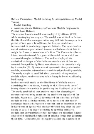
  • 18. the prospective values, and finally choosing the optimal settings. Below is a flow chart that accentuates this approach. c. Model Validation The major benefit of employing logistic regression model is the simplicity in the results interpretation through the use of odd ratios (Han et al., 2018). Besides, logistic regression is a studier technique for models that are dependent on binomial outcomes that make use of numerous descriptive aspects. Furthermore, since normal regression does not uphold the assumption of ordinariness in the event of unqualified output variable, logistic regression deals with this concern through provision of a model that reflects the non-linear output in a linear manner within the boundaries of 0 and 1. Since loan lending plays a critical role in global finance, credit scoring is a vital technique of evaluating the credit risk. Most previous researches made use of numerous mechanical learning techniques which included Neural Networks, Decision trees, logistic regression as well as support vector machine. Every mechanical learning algorithm demonstrated accuracy and instrumental in many environments. While many studies emphasized on accurateness for the forecast of loan default uncovering, it was evident that few researches put focus on the consequences of false negatives which proves to be considerably overwhelming to the lending banks. Upon selecting a prospect range of parameters, a dependable prediction of model performance is then attained. The performance on the present samples is then amassed into performance outlook which is subsequently employed in establishing the final tuning parameters. The final model is then formulated encapsulating all the default data through the tuning parameters. The loan default data can then be re-sampled as assessed numerous times for every tuning parameter point. The
  • 19. resultant values are then amassed in an effort to obtain the optimal value of K. The technique outlined in the flow chart presented above makes use of prospect models that are subject to the tuning parameters. Mitchell (1998) has proposed another technique known as genetic algorithms while Olsson & Nelson (1975) proposed the simplex search method. These two techniques are useful in determining the most favorable tuning parameters. These approaches establish the apposite values for tuning parameters algorithmically, and iterate up until they attain a parameter situation with most advantageous performance. The approaches lean towards assessing a huge number of prospect models and offer superior results compared to an established range of tuning parameters in the event that the model performance is effectively computed References Aggarwal, C.C. (2012), A Segment-Based Framework For Modeling And Mining Data Streams. Knowledge and inf. Sys. 30(1), 1–29 Akkoc, S., 2012. An Empirical Comparison of Conventional Techniques, Neural Networks and the Three Stage Hybrid Adaptive Neuro Fuzzy Inference System (Anfis) Model for Credit Scoring Analysis: The Case of Turkish Credit Card Data.
  • 20. European Journal of Operational Research, 222(1): 168–178. Alexander B. (2012), Determinant of Bank Failures the Case of Russia, Journal of Applied Statistics, 78 (32), 235-403. Anatoly B. J (2014). The probability of default models of Russian banks. Journal of Institute of Economics in Transition 21 (5), 203-278. Altman E. (1968), Financial Ratios, Discriminant Analysis, and Prediction of Corporate Bankruptcy, Journal of Finance 23 (4) 589-609. Beirlant, (2004), Statistics of extremes, Hoboken, NJ: Wiley. Calabrese, R. (2012). Modeling SME Loan Defaults as Rare Events: The Generalized Extreme Value Regression, Journal of Applied Statistics, 00 (00), 1-17. Coles, S. (2001). An Introduction to Statistical Modeling of Extreme Values, London: Springer. Gilli, M., & KeÌllezi, E. (2000). Extreme Value Theory for Tail- Related Risk Measures, Geneva: FAME. Goodhart, C. (2011). The Basel Committee on Banking Supervision, Cambridge: Cambridge University Press Han, J.T., Choi, J.S., Kim, M.J. and Jeong, J., (2018). Developing a Risk Group Predictive Model for Korean Students Falling Into Bad Debt, Asian Economic Journal, 32(1), pp.3–14. Thomas, L., 2000. A Survey of Credit And Behavioral Scoring: Forecasting Financial Risk Of Lending To Consumers. Int. J. Forecast, 16(2): 149–172. Rafaella, C. Giampiero, M. (n.d.). Bankruptcy Prediction Of Small And Medium Enterprises Using S Flexible Binary GEV Extreme Value Model, American Journal of Theoretical and Applied Statistics, 1307 (2), 3556-3798. Singhee, A., & Rutenbar, R. (2010) Extreme Statistics In Nanoscale Memory Design. New York: Springer. Yap, P., S. Ong and N. Husain (2011). Using Data Mining to Improve Assessment of Credit Worthiness via Credit Scoring Models, Exp. Syst. Appl, 38(10): 1374–1383. Yang, D., Rundensteiner, E.A., Ward, M.O. (2009). Neighbor- Based Pattern Detection For Windows Over Streaming Data. In:
  • 21. Advances in DB Tech., pp. 529–540. ACM Defining Variables for Tuning Parameters Data Re-sampling, Model Fitting, and Hold-outs Prediction Aggregating Re-sampling into Performance Profiles Final Tuning Parameters Applying Final Tuning Parameters and Refitting the Model Mass holder = 50.5 g Lane = 30.5 cm M1 = 15.5g L1 = 48.1 cm
  • 22. M2= 200.5 g L2= 52.3 cm M3= 250.5g L3= 56.5cm The Spring-Mass Oscillator Goals and Introduction In this experiment, we will examine and quantify the behavior of the spring-mass oscillator. The spring-mass oscillator consists of an object that is free to oscillate up and down, suspended from a spring (Figure 19.1). The periodic motion of the object attached to the spring is an example of harmonic motion – a motion for which the acceleration is always directed oppositely from the displacement of the object from an equilibrium position. When an object with mass m is hung from a spring with spring constant k, the spring stretches, changing its length by an amount x. When motionless, the spring-mass system is in equilibrium.
  • 23. There is a gravitational force pulling down on the mass and the spring restoring force pulling up on the mass. The spring restoring force is given by springF kx , (Eq. 1) where the k is the spring constant in units of N/m and x is the extension or compression of the spring from its natural length. The displacement, x, could be positive or negative depending on whether the spring is compressed or stretched (we would need to decide the direction of the positive x-axis). The minus sign in Eq. 1 indicates that the direction of the spring restoring force always opposes the direction of the displacement from the equilibrium position. We can say in general, however, that when the spring-mass system is in equilibrium, spring gravityF F , or kx mg . In Figure 19.1, we see an example of a spring-mass system where the equilibrium position above the location of a detector is noted. It is displacement from this
  • 24. equilibrium position that will then cause the system to oscillate. If the object, or mass, is pulled downwards a distance A from the equilibrium position and then released, the spring restoring force will initially cause the object to accelerate upwards. This would continue until the object moves above the equilibrium position, and the spring compresses past that point. The spring is then pushing downwards on the object to try to get it back to the equilibrium position, and it begins to slow down. You might say that when the object is displaced from the equilibrium position and released, it is always being pushed or pulled by the spring in an effort to return it to the equilibrium position. In simple harmonic motion, the displacement of the object from the equilibrium position will behave sinusoidally. This means that when we graph the position of the object over time while it oscillates, we should see a curve that is similar to a sine or cosine function. This is also true for the velocity and the acceleration of the object over time. If the positive x-axis points upwards in
  • 25. Figure 19.1 our picture, the position of the object will first have a value less than the equilibrium position, begin to increase, reach some maximum value a distance A above the equilibrium position, and then decrease until it returns to the release point, a distance A below the equilibrium position. The motion is symmetric, as indicated in Figure 19.1. One can find a similar oscillatory behavior for the velocity and acceleration, but they are not in sync with each other or with the position as a function of time. In other words, just because the position is increasing and “positive” (above the equilibrium position) does not mean that the velocity is also increasing and positive (above a velocity of 0). There are some expected features of simple harmonic motion for the spring-mass system that we should verify in any data set before proceeding with further analysis. A detector will be placed
  • 26. below the spring-mass system and will be used to collect data on the position, velocity and acceleration of the mass as a function of time, while it is oscillating. The data will be displayed as three graphs and the following behaviors should be observed in these graphs: 1) When the object reaches a maximum position (either above or below the equilibrium point), the velocity should be 0 at that instant. 2) When the object reaches a maximum position (either above or below the equilibrium point), the acceleration should be at an extreme. In other words, the acceleration should be at its maximum positive or maximum negative value (depends on the direction of the spring restoring force at that instant) 3) When the object is at the equilibrium position (moving through it), the velocity should be at a maximum. In other words, the velocity should be at its maximum positive or
  • 27. maximum negative value (depends on whether it is moving up or down at that instant) 4) When the object is at the equilibrium position (moving through it), the acceleration should be 0 at that instant. This is because the spring is back to a length where its restoring force is equal to the gravitational force on the object. It is also worth noting that once the spring-mass system is set into motion, we expect that the total mechanical energy, E, of the system should be conserved. This is because the spring restoring force is a conservative force, like the gravitational force. For small oscillations, we can ignore the gravitational potential energy and approximate the total energy in the spring-mass system as 2 21 1 2 2 springE KE PE mv kx (Eq. 2) where x is the amount of compression or stretch of the spring
  • 28. measured from the equilibrium position. This means that during the motion, x will never be bigger than A, the amplitude of the motion. Because the total mechanical energy should be conserved, it should be the case that if we calculate E at different moments in time, it should be the same. Another interesting aspect of this simple harmonic motion can be found by further examining the relationship between the position and acceleration as functions of time. The time it takes the spring-mass to go through one complete oscillation (from one extreme position to the other, and then back to the starting extreme) is called the period, T. Therefore, the period can be found from the position vs. time (or x vs. t) graph. If we look at the amount of time that has passed from one peak to the next on the plot (remember it will look like a sine function), this should be equal to the period! The object is leaving a position and arriving there again, moving in the same
  • 29. direction, at a later time; one cycle has been completed. An event that is periodic may also be described in terms of its frequency, f, or how many times the oscillation repeats per second. The period and frequency of an oscillation are related: 1 f T . (Eq. 3) Careful analysis suggests that the period, and thus the frequency, is dependent upon the spring constant, k, and the mass of the object, m. The prediction is that the frequency for the simple harmonic motion of a spring-mass system should be given by 1 2 k f m . (Eq. 4)
  • 30. Note that this frequency is independent of the amplitude of the motion! Here, we intend to measure the period of the spring-mass system, the spring constant, and the mass of the object in an effort to confirm the validity of the relationship in Eq. 4. Along the way, we also hope to verify the predicted sinusoidal behavior of the three kinematic quantities (position, velocity, and acceleration) and investigate the conservation of energy that should be evident during the motion. Goals: (1) Measure and consider aspects of the spring-mass oscillator. (2) Test the validity of the Eq. 4 by measuring the period, spring constant, and mass. (3) Verify the sinusoidal behavior of the kinematic quantities of the spring-mass oscillator. (4) Verify the conservation of energy during the motion of the oscillator.
  • 31. Procedure Equipment – spring, mass holder with removable masses, meter stick (or other distance- measurement tool), balance, motion detector, computer with the DataLogger interface and LoggerPro software The basic setup should be completed for you prior to lab, as shown in Figure 19.1. We will need to calibrate this using the following steps (if there is no setup, your TA should aid the class in getting to this calibration point). The motion detector should be on the floor with a protective shield over it. Above the detector, the mass holder will hang from the spring. 1) Measure and record the mass of the mass holder, using the balance. Label this as mholder. 2) If it is not already done, hang the spring from the support that should be setup for you. Be sure that the large end of the spring is on top. Measure and record the length of the spring with
  • 32. nothing attached to it. Be sure to measure from the first coil on top to the last coil on the bottom. Label this as Lspring. 3) Before starting, check to see that the motion detector cable is connected to DIG/Sonic #1 of the DataLogger interface box, and that the interface unit is turned on. If you are unsure, check with your TA. 4) Click on the link on the lab website to open LoggerPro. You should see three graphs – x vs. t, v vs. t, and a vs. t. 5) Position the motion detector on the floor directly under the spring. Do this by sighting through the spring from above to locate the appropriate position of the detector on the floor. This is important because the detector needs to “see” the mass you will hang throughout the motion. 6) Attach the mass holder to the bottom end of the spring and add a 100-g mass to the mass holder.
  • 33. 7) One partner should operate the computer and the other should pull the mass downwards about 10 cm. 8) As one partner releases the mass (do not push it – just let it go), the other should hit the green button on the top-center of the screen in LoggerPro (each time you hit the green button, the pervious plots are erased and new ones are created). Verify that the graphs appear similar to sine or cosine curves, so that the detector is “seeing” the object clearly. You can stop the data collection by hitting the red button (where the green button was). 9) Take the time now to adjust the axes of any of the graphs so the data appear clearly on each graph. This can be accomplished by double-clicking on any of the graphs and adjusting the max or min range for the vertical axis. Click on “Axes Options”. You should adjust the axes so the data fills each graph as much as possible, but is still visible.
  • 34. Upon completion of step 9, you should be calibrated. BE CAREFUL not to bump the detector or the table. If you do, realignment will likely be required. Recall that when the system is in equilibrium, the gravitational force on the mass will be equal to the spring restoring force. We can use this fact to calculate the value of the spring constant later, using the following set of data: 10) You should currently have the mass holder on the spring with a 100-g mass on its base. Record the current total mass (mass plus the holder) and label it as m1. 11) Be sure that the spring-mass system is in equilibrium and not moving. When it is, measure and record the length of the spring, consistent with the way you measured in Step 2. Label this as L1. 12) Place a 50-g mass on the mass holder, adding it to the 100-g mass already there. Record the
  • 35. new total mass (mass plus the holder) and label it as m2. 13) Be sure that the spring-mass system is in equilibrium. When it is, measure and record the length of the spring. Label this as L2. 14) Place another 50-g mass on the mass holder. Record the new total mass (mass plus the holder) and label it as m3. 15) Be sure that the spring-mass system is in equilibrium. When it is, measure and record the length of the spring. Label this as L3. Now, we will create the graphs for the oscillation of this spring- mass system. From these, we can test for the four expected behaviors of this motion (see the Lab Introduction), measure the amplitude of the motion, and measure the period of the motion. 16) Again, have one partner operate the computer and the other pull the mass. Pull the mass downwards about 10 cm.
  • 36. 17) Create your three graphs for analysis. As one partner releases the mass (do not push it – just let it go), the other should hit the green button on the top-center of the screen in LoggerPro. Allow the data collection to run for several seconds so that you get a decent number of cycles recorded (at least four). When you are ready to stop the data collection, hit the red button. 18) Be sure to adjust the axes again, if necessary, so that the data fill each window without being clipped. Also check and verify that the four expected behaviors (see the Lab Introduction) are evident in your data. If they are not, it is possible that the detector “lost” the mass briefly, or another significant source of error has interfered. Create a new set of graphs in that case. When you are happy with the appearance of your graphs, Print a copy for each partner. Label your graphs with “200 g” to note the additional mass that was on the holder when you made these graphs.
  • 37. 19) Remove two 50-g masses so the mass holder contains only 100 g of additional mass. Switch partner positions (the mass operator should now operate the computer, and vice versa) and repeat steps 16-18 to produce another set of plots. Be sure to label the plots made with “100 g” versus the “200 g”, so you don’t confuse them with the plots you created the first time. As always, be sure to organize your data records for presentation in your lab report, using tables and labels where appropriate. Data Analysis Consider the stretched spring lengths L1, L2, and L3. Compute the elongation of the spring in each case: xi = Li - Lspring, where i = 1, 2, and 3. In each case, there was an associated mass hanging on the spring, m1, m2, or m3. Using the mass for each case and the amount of stretch x you have calculated, find a value for the spring constant in each case. Recall from the introduction that in equilibrium, spring gravityF F , or kx mg (g =
  • 38. 9.8 m/s 2 ) . Label each of your results as k1, k2, and k3. Average your results for k and label this as kavg. This is the value of k we will use for the spring- mass system for all further calculations. Examine your graph for the position vs. time when there was 200 g of additional mass on the mass holder. Use the graph to determine the amplitude, A, and record your result. Consider Figure 9.1 for aid in thinking about the measurement. The amplitude is the greatest distance from the equilibrium position the object had during the motion. Question 1: Is your amplitude close to 10 cm? Why might we expect this to be about 10 cm? Examine each of your graphs for when there was 200 g of additional mass on the mass holder and, again, verify that the four expected behaviors of the motion are represented. Question 2: Identify examples of moments in time from your
  • 39. graphs when each of the four behaviors are evident (these will not all happen at the same time, but a couple might!). Mark these moments in time on your graphs using a “ ” along each curve. In answering this question, quote the relevant times you have chosen, describe what behaviors are present at each time, and explain why your results do or do not make sense. What is the spring-mass system doing at these moments in time? Note that when you made these graphs the additional mass was 200 g. Also, we are using kavg as our value for k, and the value for x in any of our equations is the displacement of the mass from the equilibrium position. Choose a moment in time when the object is at a maximum displacement. At this moment x = A. What is v at this moment? Calculate the total energy at this moment using Eq. 2. Label this energy as E1.
  • 40. Choose another moment in time when the object is moving at a maximum velocity. What is the displacement of the object from the equilibrium position at this time? Is it zero like it should be? Calculate the total energy at this moment using Eq. 2. Label this energy as E2. Choose another moment in time when the object is neither at its maximum position nor its maximum velocity. What is the velocity at this moment? What is the displacement of the object from the equilibrium position at this time? Calculate the total energy at this moment using Eq. 2. Label this energy as E3. Later we will evaluate these conservation of energy calculations. Examine your graph for the position vs. time again, when there was 200 g of additional mass on the mass holder. Use the graph to determine the period, T, and record your result. Recall that the period is the time it takes for the object to go through one complete cycle of its motion. This is represented by the time between peaks on the position vs. time graph.
  • 41. Calculate the frequency of the motion using your period and Eq. 3. Label this as factual200. Note that the frequency will have units of 1/s, often called Hertz (Hz). Now, use Eq. 4, the kavg you calculated, and the mass of the object when you made your graphs (should have been m3) to calculate the predicted frequency. Label your result as fpredict200. Finally, consider the graphs that you made with 100 g of additional mass on the mass holder. From these graphs, determine the period of the oscillation, and calculate its frequency using this period and Eq. 3. Label this as factual100. Question 3: Is the amplitude of the position graph with the 100 g on the mass holder similar to that on the position graph using 200 g on the mass holder? Should it be? Explain why or why not. Then, compare the value of the frequencies you calculated in the two cases. Are they the same? Why or why not? Consider Eq. 4 when answering.
  • 42. Error Analysis Consider the total energies you calculated (E1, E2, and E3). Find the percent difference between each of these energies. You should have three results here – one for each pair of energies. The percent difference between any of the two energies is given by: %diff 100% ( ) 2 i j ij i j E E E E This is very similar to percent error except we are dividing by the average of the two quantities since we do not have an “accepted” value for comparison.
  • 43. Question 4: Was energy conserved during the motion? Explain your conclusion based on your data. Consider your results for the frequencies you found, factual200 and fpredict200. Find the percent error of the measured frequency factual200 compared to the expected frequency fpredict200. Question 5: Remember that we found fpredict200 from Eq. 4. Comment on the validity of Eq. 4, given your measurements and comparison and explain your conclusion. Questions and Conclusions Be sure to address Questions 1-5 and describe what has been verified and tested by this experiment. What are the likely sources of error? Where might the physics principles investigated in this lab manifest in everyday life, or in a job setting? Pre-Lab Questions
  • 44. Please read through all the instructions for this experiment to acquaint yourself with the experimental setup and procedures, and develop any questions you may want to discuss with your lab partner or TA before you begin. Then answer the following questions and type your answers into the Canvas quiz tool for “The Spring-Mass Oscillator,” and submit it before the start of your lab section on the day this experiment is to be run. PL-1) A spring that hangs vertically is 25 cm long when no weight is attached to its lower end. Steve adds 250 g of mass to the end of the spring, which stretches to a new length of 37 cm. What is the spring constant, k, in N/m? PL-2) Students performing this experiment use Eq. 4 to calculate the frequency of oscillation of their mass to be 0.65 s -1 (that is, 0.65 Hz). Predict the time, in seconds, between successive peaks
  • 45. in the position vs. time plot they should expect to obtain when they measure the oscillation. A mass and holder with a total mass of 350 g is hung at the lower end of a spring with a spring constant k of 53.0 N/m. The mass is pulled down 7.0 cm below the equilibrium point and released, setting the mass-spring system into simple harmonic. [Use these data to answer questions PL-3 through PL-5]. PL-3) What is the frequency of this motion in Hertz? PL-4) What is the total mechanical energy in the spring-mass system, in Joules, at the moment it is released? PL-5) After the mass is released, its position and velocity change as the potential energy of the system is converted into the kinetic energy of the mass. At some point, all of the mechanical energy is in the form of kinetic energy (the mass has its maximum velocity), and the potential energy of the spring-mass is zero. Now, imagine you stopped the mass, then restarted the
  • 46. oscillation by pulling the mass 9.0 cm below the equilibrium point. The maximum velocity the mass obtains will be (A) larger, because more potential energy is stored in the system so more kinetic energy results. (B) larger, because the velocity of the initial pull adds to the second pull. (C) smaller, because more potential energy is stored in the system so less kinetic energy results. (D) smaller, because the mass starts at a lower position, so its peak velocity will be lower. (E) the same, because energy is conserved.
  • 47. IMG-0250.pdf (p.1)IMG-0251.pdf (p.2)IMG-0252.pdf (p.3)IMG-0253.pdf (p.4)IMG-0254.pdf (p.5)IMG-0255.pdf (p.6)IMG-0256.pdf (p.7)IMG-0257.pdf (p.8)IMG-0258.pdf (p.9)IMG-0259.pdf (p.10)IMG-0260.pdf (p.11)IMG-0261.pdf (p.12)IMG-0262.pdf (p.13)IMG-0263.pdf (p.14)IMG-0264.pdf (p.15)IMG-0265.pdf (p.16)IMG-0266.pdf (p.17) 1. Exploratory Analysis (45 Marks) · Exploratory Analysis of data & an executive summary of your top findings, supported by graphs. 15 Marks · What kind of trends do you notice in terms of consumer behavior over different times of the day and different days of the week? Can you give concrete recommendations based on the same? 10 Marks · Are there certain menu items that can be taken off the menu? 10 Marks
  • 48. · Are there trends across months that you are able to notice? 10 Marks 2. Menu Analysis- (45 Marks) · Identify the most popular combos that can be suggested to the restaurant chain after a thorough analysis of the most commonly occurring sets of menu items in the customer orders. The restaurant doesn’t have any combo meals. Can you suggest the best combo meals? 45 Marks Please note the following: · Your submission:should be a PowerPoint Presentation (Deck of 19- 20 slides). Appendices are not counted in the word limit. · You must give the sources of data presented. Do not refer to blogs; Wikipedia etc. · Please ensure timely submission as post-deadline assignment will not be accepted. Scoring guide (Rubric) - Rubric (3) Criteria Points Exploratory Analysis of data & executive summary of your top findings, supported by graphs.f criterion 15 What kind of trends do you notice in terms of consumer behavior over different times of the day and different days of the week? Can you give concrete recommendations based on the same? on 10 Are there certain menu items that can be taken off the menu? 10 Are there trends across months that you are able to notice?erion 10 Identify the most popular combos that can be suggested to the restaurant chain after a thorough analysis of the most commonly occurring sets of menu items in the customer orders. The restaurant doesn’t have any combo meals. Can you suggest the best combo meals? 45