This document is the table of contents for the book "Python Programming and Numerical Methods: A Guide for Engineers and Scientists". It outlines the book's contents which cover topics such as Python basics, variables and data structures, functions, branching statements, iteration, recursion, and object-oriented programming. The book is intended as a guide for engineers and scientists to learn Python programming and numerical methods.


![Fig. 20.2 Finite difference approximation of the derivative. 339
Fig. 20.3 Illustration of the forward difference, the backward difference, and the central difference. Note
the difference in slopes depending on the method used. 341
Fig. 21.1 Illustration of the integral. The integral from a to b of the function f is the area below the curve
(shaded in grey). 353
Fig. 21.2 Illustration of the trapezoid integral procedure. The area below the curve is approximated by a
sum of areas of trapezoids that approximate the function. 357
Fig. 21.3 Illustration of the Simpson integral formula. Discretization points are grouped by three, and a
parabola is fit between the three points. This can be done by a typical interpolation polynomial.
The area under the curve is approximated by the area under the parabola. 360
Fig. 21.4 Illustration of the accounting procedure to approximate the function f by the Simpson rule for
the entire interval [a,b]. 361
Fig. 22.1 Pendulum system. 372
Fig. 22.2 The illustration of the explicit Euler method. 376
Fig. 22.3 The illustration of the stiffness equation. 390
Fig. 23.1 Heat flow in a pin fin. The variable L is the length of the pin fin, which starts at x = 0 and
finishes at x = L. The temperatures at two ends are T0 and TL, with Ts being the surrounding
environment temperature. 400
Fig. 23.2 Target shooting analogy to the shooting method. 401
Fig. 23.3 Illustration of the finite difference method. 406
Fig. 24.1 Period and amplitude of a sine wave. 418
Fig. 24.2 Wavelength and amplitude of a sine wave. 418
Fig. 24.3 More general wave form. 422
Fig. 24.4 Illustration of Fourier transform with time and frequency domain signal. 422
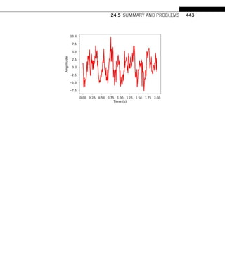
Fig. 24.5 Signal generated before with 3 frequencies. 433
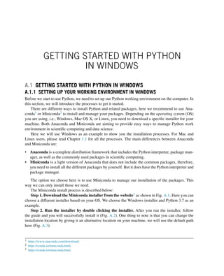
Fig. A.1 The Miniconda download page, choose the installer based on your operating system. 446
Fig. A.2 Screen shot of running the installer in Anaconda prompt. 446
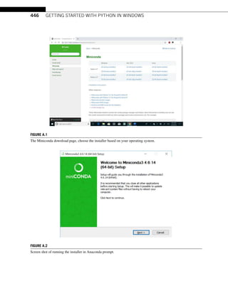
Fig. A.3 The default installation location of your file system. 447
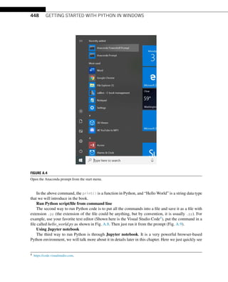
Fig. A.4 Open the Anaconda prompt from the start menu. 448
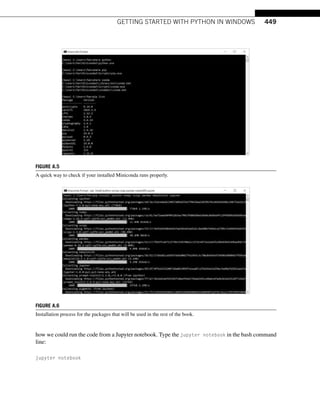
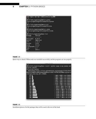
Fig. A.5 A quick way to check if your installed Miniconda runs properly. 449
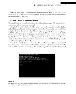
Fig. A.6 Installation process for the packages that will be used in the rest of the book. 449
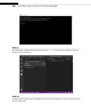
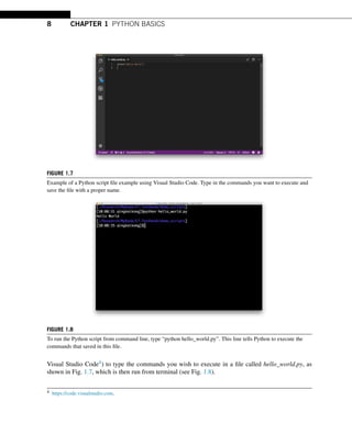
Fig. A.7 Run "Hello World" in IPython shell by typing the command, “print” is a function that we will
learn to print out anything within the parentheses. 450
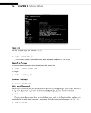
Fig. A.8 A Python script file example using Visual Studio Code. You type in the commands you want to
execute and save the file with a proper name. 450
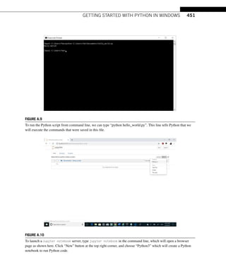
Fig. A.9 To run the Python script from command line, we can type “python hello_world.py”. This line
tells Python that we will execute the commands that were saved in this file. 451
Fig. A.10 To launch a Jupyter notebook server, type jupyter notebook in the command line, which
will open a browser page as shown here. Click “New” button at the top right corner, and choose
“Python3” which will create a Python notebook to run Python code. 451
Fig. A.11 Run the Hello World example within Jupyter notebook. Type the command in the code cell
(the grey boxes) and press Shift + Enter to execute it. 452](https://image.slidesharecdn.com/pythonprogrammingandnumericalmethodsaguideforengineersand-231017183839-0fbc5295/85/Python_Programming_and_Numerical_Methods_A_Guide_for_Engineers_and-pdf-13-320.jpg)
![1.2 PYTHON AS A CALCULATOR 9
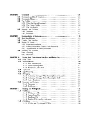
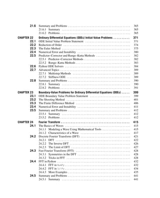
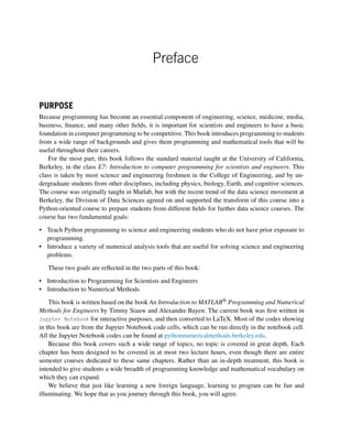
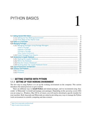
FIGURE 1.9
To launch a Jupyter notebook server, type jupyter notebook in the command line, which will open a browser
page as shown here. Click the “New” button on the top right and choose “Python3”. This will create a Python
notebook from which to run Python code.
Using Jupyter Notebook. The third way to run Python is through Jupyter Notebook, which is a very
powerful browser-based Python environment. We will discuss this in details later in this chapter. The
example presented here is to demonstrate how quickly we can run the code using Jupyter notebook.
If you type jupyter notebook in the terminal, a local web page will pop up; use the upper right button
to create a new Python3 notebook, as shown in Fig. 1.9.
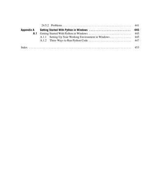
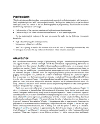
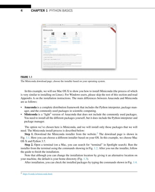
Running code in Jupyter notebook is easy. Type your code in the cell and press Shift + Enter
to run the cell; the results will be shown below the code (Fig. 1.10).
1.2 PYTHON AS A CALCULATOR
Python contains functions found in any standard graphing calculator. An arithmetic operation is either
addition, subtraction, multiplication, division, or powers between two numbers. An arithmetic opera-
tor is a symbol that Python has reserved to mean one of the aforementioned operations. These symbols
are + for addition, - for subtraction, * for multiplication, / for division, and ** for exponentiation.
An instruction or operation is executed when it is resolved by the computer. An instruction is
executed at the command prompt by typing it where you see the >>> symbol appears in the Python
shell (or the In [1]: sign in IPython) and then pressing Enter. In the case of the Jupyter notebook,
type the operation in the code cell and Shift + Enter. Since we will use Jupyter notebook for the
rest of the book, to familiarize yourself with all the different options, all examples in this section will
be shown in the IPython shell – see the previous section for how to begin working in IPython. For
Windows users, you will use the Anaconda prompt shown in the Appendix A instead of using the
terminal.](https://image.slidesharecdn.com/pythonprogrammingandnumericalmethodsaguideforengineersand-231017183839-0fbc5295/85/Python_Programming_and_Numerical_Methods_A_Guide_for_Engineers_and-pdf-24-320.jpg)
![10 CHAPTER 1 PYTHON BASICS
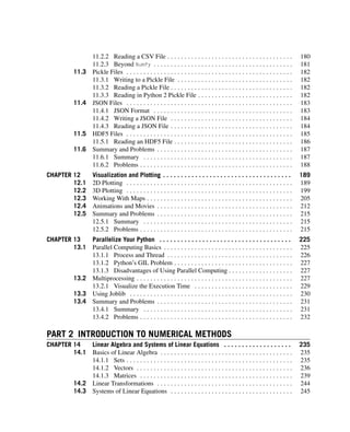
FIGURE 1.10
To run the Hello World example within Jupyter notebook, type the command in the code cell (the grey boxes) and
press Shift + Enter to execute it.
TRY IT! Compute the sum of 1 and 2.
In [1]: 1 + 2
Out[1]: 3
An order of operations is a standard order of precedence that different operations have in re-
lationship to one another. Python utilizes the same order of operations you learned in grade school.
Powers are executed before multiplication and division, which are executed before addition and
subtraction. Parentheses () can also be used in Python to supersede the standard order of opera-
tions.
TRY IT! Compute 3×4
(22+4/2)
.
In [2]: (3*4)/(2**2 + 4/2)
Out[2]: 2.0
TIP! Note that Out[2] is the resulting value of the last operation executed. Use the underscore
symbol _ to represent this result to break up complicated expressions into simpler commands.](https://image.slidesharecdn.com/pythonprogrammingandnumericalmethodsaguideforengineersand-231017183839-0fbc5295/85/Python_Programming_and_Numerical_Methods_A_Guide_for_Engineers_and-pdf-25-320.jpg)
![1.2 PYTHON AS A CALCULATOR 11
TRY IT! Compute 3 divided by 4, then multiply the result by 2, and then raise the result to the
3rd power.
In [3]: 3/4
Out[3]: 0.75
In [4]: _*2
Out[4]: 1.5
In [5]: _**3
Out[5]: 3.375
Python has many basic arithmetic functions like sin, cos, tan, asin, acos, atan, exp, log, log10,
and sqrt stored in a module (explained later in this chapter) called math. First, import this module to
access to these functions.
In [6]: import math
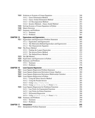
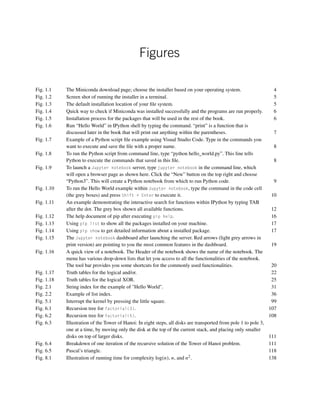
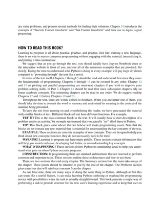
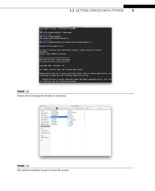
TIP! In Jupyter notebook and IPython, you can have a quick view of what is in the module
by typing the module name + dot + TAB. Furthermore, if you type the first few letters of the
function and press TAB, it will automatically complete the function, which is known as “TAB
completion” (an example is shown in Fig. 1.11).
These mathematical functions are executed via module.function. The inputs to them are always
placed inside of parentheses that are connected to the function name. For trigonometric functions, it is
useful to have the value of π available. You can call this value at any time by typing math.pi in the
IPython shell.
TRY IT! Find the square root of 4.
In [7]: math.sqrt(4)
Out[7]: 2.0
TRY IT! Compute the sin(π
2 ).
In [8]: math.sin(math.pi/2)
Out[8]: 1.0
Python composes functions as expected, with the innermost function being executed first. The same
holds true for function calls that are composed with arithmetic operations.](https://image.slidesharecdn.com/pythonprogrammingandnumericalmethodsaguideforengineersand-231017183839-0fbc5295/85/Python_Programming_and_Numerical_Methods_A_Guide_for_Engineers_and-pdf-26-320.jpg)
![12 CHAPTER 1 PYTHON BASICS
FIGURE 1.11
An example demonstrating the interactive search for functions within IPython by typing TAB after the dot. The grey
box shown all available functions.
TRY IT! Compute elog 10.
In [9]: math.exp(math.log(10))
Out[9]: 10.000000000000002
Note that the log function in Python is loge, or the natural logarithm. It is not log10. To use log10,
use the function math.log10.
TIP! You can see the result above should be 10, but in Python, it shows as 10.000000000000002.
This is due to Python’s number approximation, discussed in Chapter 9.
TRY IT! Compute e
3
4 .
In [10]: math.exp(3/4)
Out[10]: 2.117000016612675
TIP! Using the UP ARROW in the command prompt recalls previously executed commands that
were executed. If you accidentally type a command incorrectly, you can use the UP ARROW to
recall it, and then edit it instead of retyping the entire line.
Often when using a function in Python, you need help specific to the context of the function. In
IPython or Jupyter notebook, the description of any function is available by typing function?; the](https://image.slidesharecdn.com/pythonprogrammingandnumericalmethodsaguideforengineersand-231017183839-0fbc5295/85/Python_Programming_and_Numerical_Methods_A_Guide_for_Engineers_and-pdf-27-320.jpg)
![1.2 PYTHON AS A CALCULATOR 13
question mark is a shortcut for help. If you see a function you are unfamiliar with, it is good practice
to use the question mark before asking your instructors what a specific function does.
TRY IT! Use the question mark to find the definition of the factorial function.
In [11]: math.factorial?
Signature: math.factorial(x, /)
Docstring:
Find x!.
Raise a ValueError if x is negative or non-integral.
Type: builtin_function_or_method
Python will raise an ZeroDivisionError when the expression 1/0 (which is infinity) appears, to
remind you.
TRY IT! 1/0.
In [12]: 1/0
----------------------------------------------------------------------
ZeroDivisionError Traceback (most recent call last)
<ipython-input-12-9e1622b385b6> in <module>()
----> 1 1/0
ZeroDivisionError: division by zero
You can type math.inf at the command prompt to denote infinity or math.nan to denote something
that is not a number that you wish to be handled as a number. If this is confusing, this distinction can be
skipped for now; it will be explained in detail later. Finally, Python can also handle imaginary numbers.
TRY IT! Type 1/∞, and ∞ ∗ 2 to verify that Python handles infinity as you would expect.
In [13]: 1/math.inf
Out[13]: 0.0
In [14]: math.inf * 2
Out[14]: inf
TRY IT! Compute ∞/∞.
In [15]: math.inf/math.inf
Out[15]: nan](https://image.slidesharecdn.com/pythonprogrammingandnumericalmethodsaguideforengineersand-231017183839-0fbc5295/85/Python_Programming_and_Numerical_Methods_A_Guide_for_Engineers_and-pdf-28-320.jpg)
![14 CHAPTER 1 PYTHON BASICS
TRY IT! Compute sum 2 + 5i.
In [16]: 2 + 5j
Out[16]: (2+5j)
Note that in Python the imaginary part is represented by j instead of i.
Another way to represent a complex number in Python is to use the complex function.
In [17]: complex(2,5)
Out[17]: (2+5j)
Python can also handle scientific notation using the letter e between two numbers. For example,
1e6 = 1000000 and 1e − 3 = 0.001.
TRY IT! Compute the number of seconds in 3 years using scientific notation.
In [18]: 3e0*3.65e2*2.4e1*3.6e3
Out[18]: 94608000.0
TIP! Every time a function in math module is typed, it is always typed math.function_name.
Alternatively, there is a simpler way. For example, if we want to use sin and log from math
module, we can import them as follows: from math import sin, log. With this modified import
statement, when using these functions, use them directly, e.g., sin(20) or log(10).
The previous examples demonstrated how to use Python as a calculator to deal with different data
values. In Python, there are additional data types needed for numerical values: int, float, and complex
are the types associated with these values.
• int: Integers, such as 1,2,3,...
• float: Floating-point numbers, such as 3.2,6.4,...
• complex: Complex numbers, such as 2 + 5j,3 + 2j,...
Use function type to check the data type for different values.
TRY IT! Find out the data type for 1234.
In [19]: type(1234)
Out[19]: int](https://image.slidesharecdn.com/pythonprogrammingandnumericalmethodsaguideforengineersand-231017183839-0fbc5295/85/Python_Programming_and_Numerical_Methods_A_Guide_for_Engineers_and-pdf-29-320.jpg)
![1.3 MANAGING PACKAGES 15
TRY IT! Find out the data type for 3.14.
In [20]: type(3.14)
Out[20]: float
TRY IT! Find out the data type for 2 + 5j.
In [21]: type(2 + 5j)
Out[21]: complex
Of course, there are other data types, such as boolean, string, and so on; these are introduced in
Chapter 2.
This section demonstrated how to use Python as a calculator by running commands in the IPython
shell. Before we move on to more complex coding, let us go ahead to learn more about the managing
packages, i.e., how to install, upgrade, and remove the packages.
1.3 MANAGING PACKAGES
One feature that makes Python really great is the various packages/modules developed by the user
community. Most of the time, when you want to apply some functions or algorithms, often you will
find multiple packages already available. All you need to do is to install the packages and use them
in your code. Managing packages is one of the most important skills you need to learn to take fully
advantage of Python. This section will show you how to manage packages in Python.
1.3.1 MANAGING PACKAGES USING PACKAGE MANAGERS
At the beginning of this book, we installed some packages using pip by typing pip install pack-
age_name. This is currently the most common and easy way to install Python packages. Pip is a package
manager that automates the process of installing, updating, and removing the packages. It can install
packages published on Python Package Index (PyPI).5 If you install Miniconda, pip will be available
for you to use as well.
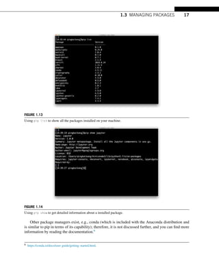
Use pip help to get help for different commands, as shown in Fig. 1.12.
The most used commands usually include: installing, upgrading, and uninstalling a package.
Install a Package
To install the latest version of a package:
pip install package_name
To install a specific version, e.g., install version 1.5:
5 https://pypi.org/.](https://image.slidesharecdn.com/pythonprogrammingandnumericalmethodsaguideforengineersand-231017183839-0fbc5295/85/Python_Programming_and_Numerical_Methods_A_Guide_for_Engineers_and-pdf-30-320.jpg)
![1.5 LOGICAL EXPRESSIONS AND OPERATORS 21
In Python, a logical expression that is true will compute to the value True. A false expression
will compute to the value False. This is a new data type known as boolean, which has the built-in
values True and False. In this book, “True” is equivalent to 1, and “False” is equivalent to 0. Logical
expressions are used to pose questions to Python. For example, “3 < 4” is equivalent to, “Is 3 less than
4?” Since this statement is true, Python will compute it as 1; however, if we write 3 > 4, this is false,
and Python will compute it as 0.
Comparison operators compare the value of two numbers, which are used to build logical expres-
sions. Python reserves the symbols >,>=,<,<=,! =,==, to denote “greater than,” “greater than or
equal,” “less than,” “less than or equal,” “not equal,” and “equal,” respectively; see and Table 1.1. Let
us start with an example, a = 4,b = 2:
Table 1.1 Comparison operators.
Operator Description Example Results
> greather than a > b True
>= greater than or equal a >= b True
< less than a < b False
<= less than or equal a <= b False
!= not equal a != b True
== equal a == b False
TRY IT! Compute the logical expression for “Is 5 equal to 4?” and “Is 2 smaller than 3?”
In [1]: 5 == 4
Out[1]: False
In [2]: 2 < 3
Out[2]: True
Logical operators, as shown in Table 1.2, are operations between two logical expressions that, for
the sake of discussion, we will call P and Q. The fundamental logical operators we will use herein are
and, or, and not.
Table 1.2 Logical operators.
Operator Description Example Results
and greater than P and Q True if both P and Q are True. False otherwise
or greater than or equal P or Q True if either P or Q is True. False otherwise
not less than not P True if P is False. False if P is True
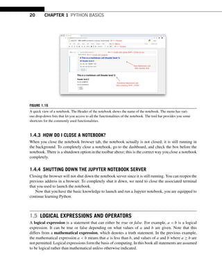
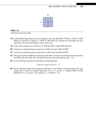
The truth table, as shown in Fig. 1.17, of a logical operator or expression gives the result of every
truth combination of P and Q. Fig. 1.17 shows the truth tables for “and” and “or”.](https://image.slidesharecdn.com/pythonprogrammingandnumericalmethodsaguideforengineersand-231017183839-0fbc5295/85/Python_Programming_and_Numerical_Methods_A_Guide_for_Engineers_and-pdf-36-320.jpg)
![22 CHAPTER 1 PYTHON BASICS
FIGURE 1.17
Truth tables for the logical and/or.
TRY IT! Assuming P is true, let us use Python to determine if the expression (P AND NOT(Q))
OR (P AND Q) is always true regardless of whether or not Q is true. Logically, can you see why
this is the case? First assume Q is true:
In [3]: (1 and not 1) or (1 and 1)
Out[3]: 1
Now assume Q is false
In [4]: (1 and not 0) or (1 and 0)
Out[4]: True
Just as with arithmetic operators, logical operators have an order of operations relative to each other
and in relation to arithmetic operators. All arithmetic operations will be executed before comparison
operations, which will be executed before logical operations. Parentheses can be used to change the
order of operations.
TRY IT! Compute (1 + 3) > (2 + 5)
In [5]: 1 + 3 > 2 + 5
Out[5]: False
TIP! Even when the order of operations is known, it is usually helpful for you and those reading
your code to use parentheses to make your intentions clearer. In the preceding example (1 + 3) >
(2 + 5) is clearer.](https://image.slidesharecdn.com/pythonprogrammingandnumericalmethodsaguideforengineersand-231017183839-0fbc5295/85/Python_Programming_and_Numerical_Methods_A_Guide_for_Engineers_and-pdf-37-320.jpg)
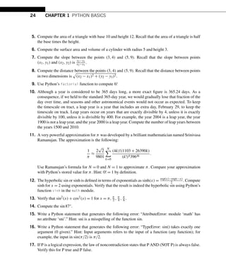
![1.6 SUMMARY AND PROBLEMS 23
WARNING! In Python’s implementation of logic, 1 is used to denote true and 0 for false. But
because 1 and 0 are still numbers, Python will allow abuses such as: (3 > 2) + (5 > 4), which will
resolve to 2.
In [6]: (3 > 2) + (5 > 4)
Out[6]: 2
WARNING! Although in formal logic 1 is used to denote true and 0 to denote false, Python’s
notation system is different, and it will take any number not equal to 0 to mean true when used
in a logical operation. For example, 3 and 1 will compute to true. Do not utilize this feature of
Python. Always use 1 to denote a true statement.
TIP! A fortnight is a length of time consisting of 14 days. Use a logical expression to determine
if there are more than 100,000 seconds in a fortnight.
In [7]: (14*24*60*60) > 100000
Out[7]: True
1.6 SUMMARY AND PROBLEMS
1.6.1 SUMMARY
1. You have now learned the basics of Python, which should enable you to set up the working envi-
ronment and experiment with ways to run Python.
2. Python can be used as a calculator. It has all the functions and arithmetic operations commonly used
with a scientific calculator.
3. You can manage the Python packages using package managers.
4. You learned how to interact with Jupyter notebook.
5. You can also use Python to perform logical operations.
6. You have now been introduced to int, float, complex, string, and boolean data types in Python.
1.6.2 PROBLEMS
1. Print “I love Python” using Python Shell.
2. Print “I love Python” by typing it into a .py file and run it from command line.
3. Type import antigravity in the IPython Shell, which will take you to xkcd and enable you to
see the awesome Python.
4. Launch a new Jupyter notebook server in a folder called “exercise” and create a new Python
notebook with the name “exercise_1.” Put the rest of the problems within this notebook.](https://image.slidesharecdn.com/pythonprogrammingandnumericalmethodsaguideforengineersand-231017183839-0fbc5295/85/Python_Programming_and_Numerical_Methods_A_Guide_for_Engineers_and-pdf-38-320.jpg)
![2
VARIABLES AND BASIC DATA
STRUCTURES
2.1 Variables and Assignment ........................................................................................... 27
2.2 Data Structure – String............................................................................................... 30
2.3 Data Structure – List.................................................................................................. 35
2.4 Data Structure – Tuple ............................................................................................... 38
2.5 Data Structure – Set .................................................................................................. 40
2.6 Data Structure – Dictionary.......................................................................................... 42
2.7 Introducing NumPy Arrays ............................................................................................ 44
2.8 Summary and Problems.............................................................................................. 52
2.8.1 Summary ............................................................................................... 52
2.8.2 Problems ............................................................................................... 52
2.1 VARIABLES AND ASSIGNMENT
When programming, it is useful to be able to store information in variables. A variable is a string of
characters and numbers associated with a piece of information. The assignment operator, denoted by
the “=” symbol, is the operator that is used to assign values to variables in Python. The line x=1 takes
the known value, 1, and assigns that value to the variable with name “x”. After executing this line, this
number will be stored into this variable. Until the value is changed or the variable deleted, the character
x behaves like the value 1.
In [1]: x = 1
x
Out[1]: 1
TRY IT! Assign the value 2 to the variable y. Multiply y by 3 to show that it behaves like the
value 2.
In [2]: y = 2
y
Out[2]: 2
In [3]: y*3](https://image.slidesharecdn.com/pythonprogrammingandnumericalmethodsaguideforengineersand-231017183839-0fbc5295/85/Python_Programming_and_Numerical_Methods_A_Guide_for_Engineers_and-pdf-41-320.jpg)
![28 CHAPTER 2 VARIABLES AND BASIC DATA STRUCTURES
Out[3]: 6
A variable is like a “container” used to store the data in the computer’s memory. The name of the
variable tells the computer where to find this value in the memory. For now, it is sufficient to know
that the notebook has its own memory space to store all the variables in the notebook. As a result of
the previous example, you will see the variables x and y in the memory. You can view a list of all the
variables in the notebook using the magic command %whos (magic commands are a specialized set of
commands host by the IPython kernel and require the prefix % to specify the commands).
TRY IT! List all the variables in this notebook.
In [4]: %whos
Variable Type Data/Info
----------------------------
x int 1
y int 2
Note! The equality sign in programming is not the same as a truth statement in mathematics. In
math, the statement x = 2 declares the universal truth within the given framework, x is 2. In program-
ming, the statement x=2 means a known value is being associated with a variable name, store 2 in
x. Although it is perfectly valid to say 1 = x in mathematics, assignments in Python always go left,
meaning the value to the right of the equal sign is assigned to the variable on the left of the equal sign.
Therefore, 1=x will generate an error in Python. The assignment operator is always last in the order of
operations relative to mathematical, logical, and comparison operators.
TRY IT! The mathematical statement x = x + 1 has no solution for any value of x. In program-
ming, if we initialize the value of x to be 1, then the statement makes perfect sense. It means, “Add
x and 1, which is 2, then assign that value to the variable x”. Note that this operation overwrites
the previous value stored in x.
In [5]: x = x + 1
x
Out[5]: 2
There are some restrictions on the names variables can take. Variables can only contain alphanu-
meric characters (letters and numbers) as well as underscores; however, the first character of a variable
name must be a letter or an underscore. Spaces within a variable name are not permitted, and the
variable names are case sensitive (e.g., x and X are considered different variables).](https://image.slidesharecdn.com/pythonprogrammingandnumericalmethodsaguideforengineersand-231017183839-0fbc5295/85/Python_Programming_and_Numerical_Methods_A_Guide_for_Engineers_and-pdf-42-320.jpg)
![2.1 VARIABLES AND ASSIGNMENT 29
TIP! Unlike in pure mathematics, variables in programming almost always represent something
tangible. It may be the distance between two points in space or the number of rabbits in a popu-
lation. Therefore, as your code becomes increasingly complicated, it is very important that your
variables carry a name that can easily be associated with what they represent. For example, the
distance between two points in space is better represented by the variable dist than x, and the
number of rabbits in a population is better represented by n_rabbits than y.
Note that when a variable is assigned, it has no memory of how it was assigned. That is, if the value
of a variable, y, is constructed from other variables, like x, reassigning the value of x will not change
the value of y.
EXAMPLE: What value will y have after the following lines of code are executed?
In [7]: x = 1
y = x + 1
x = 2
y
Out[7]: 2
WARNING! You can overwrite variables or functions that have been stored in Python. For ex-
ample, the command help = 2 will store the value 2 in the variable with name help. After this
assignment help will behave like the value 2 instead of the function help. Therefore, you should
always be careful not to give your variables the same name as built-in functions or values.
TIP! Now that you know how to assign variables, it is important that you remember to never
leave unassigned commands. An unassigned command is an operation that has a result, but that
result is not assigned to a variable. For example, you should never use 2+2. You should instead
assign it to some variable x=2+2. This allows you to “hold on” to the results of previous commands
and will make your interaction with Python much less confusing.
You can clear a variable from the notebook using the del function. Typing del x will clear the
variable x from the workspace. If you want to remove all the variables in the notebook, you can use the
magic command %reset.
In mathematics, variables are usually associated with unknown numbers; in programming, variables
are associated with a value of a certain type. There are many data types that can be assigned to variables.
A data type is a classification of the type of information that is being stored in a variable. The basic
data types that you will utilize throughout this book are boolean, int, float, string, list, tuple, dictionary,
and set. A formal description of these data types is given in the following sections.](https://image.slidesharecdn.com/pythonprogrammingandnumericalmethodsaguideforengineersand-231017183839-0fbc5295/85/Python_Programming_and_Numerical_Methods_A_Guide_for_Engineers_and-pdf-43-320.jpg)
![30 CHAPTER 2 VARIABLES AND BASIC DATA STRUCTURES
2.2 DATA STRUCTURE – STRING
We have introduced the different data types, such as int, float and boolean; these are all related to single
value. The rest of this chapter will introduce you more data types so that we can store multiple values.
The data structure related to these new types are strings, lists, tuples, sets, and dictionaries. We will
start with the strings.
A string is a sequence of characters, such as Hello World we saw in Chapter 1. Strings are
surrounded by either single or double quotation marks. We can use print function to output the strings
to the screen.
TRY IT! Print I love Python! to the screen.
In [1]: print(I love Python!)
TRY IT! Assign the character S to the variable with name s. Assign the string Hello World
to the variable w. Verify that s and w have the type string using the type function.
In [2]: s = S
w = Hello World
In [3]: type(s)
Out[3]: str
In [4]: type(w)
Out[4]: str
Note! A blank space, , between Hello and World is also a type str. Any symbol can be a
character, even those that have been reserved for operators. Note that as a str, they do not perform the
same function. Although they look the same, Python interprets them completely differently.
TRY IT! Create an empty string. Verify that the empty string is an str.
In [5]: s =
type(s)
Out[5]: str
Because a string is an array of characters, it has length to indicate the size of the string. For example,
we can check the size of the string by using the built-in function len.](https://image.slidesharecdn.com/pythonprogrammingandnumericalmethodsaguideforengineersand-231017183839-0fbc5295/85/Python_Programming_and_Numerical_Methods_A_Guide_for_Engineers_and-pdf-44-320.jpg)
![2.2 DATA STRUCTURE – STRING 31
FIGURE 2.1
String index for the example of Hello World.
In [6]: len(w)
Out[6]: 11
Strings also have indexes that enables us to find the location of each character, as shown in Fig. 2.1.
The index of the position start with 0.
We can access a character by using a bracket and the index of the position. For example, if we want
to access the character W, then we type the following:
In [7]: w[6]
Out[7]: W
We can also select a sequence as well using string slicing. For example, if we want to access
World, we type the following command.
In [8]: w[6:11]
Out[8]: World
[6:11] means the start position is from index 6 and the end position is index 10. In the Python
string slicing range, the upper-bound is exclusive; this means that [6:11] will “slice” the characters
from index 6 to 10. The syntax for slicing in Python is [start:end:step], the third argument, step, is
optional. If you ignore the step argument, the default will be set to 1.
You can ignore the end position if you want to slice to the end of the string. For example, the
following command is the same as the above one:
In [9]: w[6:]
Out[9]: World
TRY IT! Retrieve the word Hello from string w.
In [10]: w[:5]
Out[10]: Hello](https://image.slidesharecdn.com/pythonprogrammingandnumericalmethodsaguideforengineersand-231017183839-0fbc5295/85/Python_Programming_and_Numerical_Methods_A_Guide_for_Engineers_and-pdf-45-320.jpg)
![32 CHAPTER 2 VARIABLES AND BASIC DATA STRUCTURES
You can also use a negative index when slicing the strings, which means counting from the end of
the string. For example, -1 means the last character, -2 means the second to last and so on.
TRY IT! Slice the Wor within the word World.
In [11]: w[6:-2]
Out[11]: Wor
TRY IT! Retrieve every other character in the variable w
In [12]: w[::2]
Out[12]: HloWrd
Strings cannot be used in the mathematical operations.
TRY IT! Use + to add two numbers. Verify that + does not behave like the addition operator,
+.
In [13]: 1 + 2
File ipython-input-13-46b54f731e00, line 1
1 + 2
ˆ
SyntaxError: invalid syntax
WARNING! Numbers can also be expressed as str. For example, x = '123' means that x is the
string 123 not the number 123. However, strings represent words or text and so should not have
addition defined on them.
TIP! You may find yourself in a situation where you would like to use an apostrophe as an str.
This is problematic since an apostrophe is used to denote strings. Fortunately, an apostrophe can
be used in a string in the following way. The backslash () is a way to tell Python this is part of the
string, not to denote strings. The backslash character is used to escape characters that otherwise
have a special meaning, such as newline, backslash itself, or the quote character. If either single
or double quote is a part of the string itself, in Python, there is an easy way to do this, you can
just place the string in double or single quotes respectively, as shown in the following example.
In [14]: don't
Out[14]: don't
One string can be concatenated to another string. For example:](https://image.slidesharecdn.com/pythonprogrammingandnumericalmethodsaguideforengineersand-231017183839-0fbc5295/85/Python_Programming_and_Numerical_Methods_A_Guide_for_Engineers_and-pdf-46-320.jpg)
![2.2 DATA STRUCTURE – STRING 33
In [15]: str_a = I love Python!
str_b = You too!
print(str_a + str_b)
I love Python! You too!
We can convert other data types to strings as well using the built-in function str. This is useful, for
example, we have the variable x which has stored 1 as an integer type, if we want to print it out directly
as a string, we will get an error saying we cannot concatenate string with an integer.
In [16]: x = 1
print(x = + x)
-------------------------------------------------------
TypeError Traceback (most recent call last)
ipython-input-16-3e562ba0dd83 in module()
1 x = 1
---- 2 print(x = + x)
TypeError: can only concatenate str (not int) to str
The correct way to do it is to convert the integer to string first, and then print it out.
TRY IT! Print out x = 1 to the screen.
In [17]: print(x = + str(x))
x = 1
In [18]: type(str(x))
Out[18]: str
In Python, string is an object that has various methods that can be used to manipulate it (this is
the so-called object-oriented programming and will be discussed later). To get access to these various
methods, use this pattern string.method_name.](https://image.slidesharecdn.com/pythonprogrammingandnumericalmethodsaguideforengineersand-231017183839-0fbc5295/85/Python_Programming_and_Numerical_Methods_A_Guide_for_Engineers_and-pdf-47-320.jpg)
![34 CHAPTER 2 VARIABLES AND BASIC DATA STRUCTURES
TRY IT! Turn the variable w to upper case.
In [19]: w.upper()
Out[19]: HELLO WORLD
TRY IT! Count the number of occurrences for letter l in w.
In [20]: w.count(l)
Out[20]: 3
TRY IT! Replace the World in variable w to Berkeley.
In [21]: w.replace(World, Berkeley)
Out[21]: Hello Berkeley
There are different ways to preformat a string. Here we introduce two ways to do it. For example,
if we have two variables name and country, and we want to print them out in a sentence, but we do not
want to use the string concatenation we used before since it will use many + signs in the string, we
can do the following instead:
In [22]: name = UC Berkeley
country = USA
print(%s is a great school in %s!%(name, country))
UC Berkeley is a great school in USA!
WHAT IS HAPPENING? In the previous example, the %s in the double quotation marks is
telling Python that we want to insert some strings at this location (s stands for string in this case).
The %(name, country) is the location where the two strings should be inserted.
NEW! There is a different way that only introduced in Python 3.6 and above, it is called f-string,
which means formated-string. You can easily format a string with the following line:
In [23]: print(f{name} is a great school in {country}.)
UC Berkeley is a great school in USA.
You can even print out a numerical expression without converting the data type as we did before.](https://image.slidesharecdn.com/pythonprogrammingandnumericalmethodsaguideforengineersand-231017183839-0fbc5295/85/Python_Programming_and_Numerical_Methods_A_Guide_for_Engineers_and-pdf-48-320.jpg)
![2.3 DATA STRUCTURE – LIST 35
TRY it! Print out the result of 3*4 directly using f-string.
In [24]: print(f{3*4})
12
By this point, we have learned about the string data structure; this is our first sequence data structure.
Let us learn more now.
2.3 DATA STRUCTURE – LIST
In the previous section, we learned that “strings” can hold a sequence of characters. Now, we are
introducing a more versatile sequential data structure in Python – list. The way to define it is to use a
pair of brackets [ ], and the elements within it are separated by commas. A list can hold any type of
data: numerical, or strings, or other types. For example,
In [1]: list_1 = [1, 2, 3]
list_1
Out[1]: [1, 2, 3]
In [2]: list_2 = [Hello, World]
list_2
Out[2]: [Hello, World]
We can put mixed types in the list as well:
In [3]: list_3 = [1, 2, 3, Apple, orange]
list_3
Out[3]: [1, 2, 3, Apple, orange]
We can also nest the lists, for example:
In [4]: list_4 = [list_1, list_2]
list_4
Out[4]: [[1, 2, 3], [Hello, World]]
The way to retrieve the element in the list is very similar to how it is done for strings, see Fig. 2.2
for the index of a string.](https://image.slidesharecdn.com/pythonprogrammingandnumericalmethodsaguideforengineersand-231017183839-0fbc5295/85/Python_Programming_and_Numerical_Methods_A_Guide_for_Engineers_and-pdf-49-320.jpg)
![36 CHAPTER 2 VARIABLES AND BASIC DATA STRUCTURES
FIGURE 2.2
Example of list index.
TRY IT! Get the 3rd element in list_3
In [5]: list_3[2]
Out[5]: 3
TRY IT! Get the first 3 elements in list_3
In [6]: list_3[:3]
Out[6]: [1, 2, 3]
TRY IT! Get the last element in list_3
In [7]: list_3[-1]
Out[7]: orange
TRY IT! Get the first list from list_4.
In [8]: list_4[0]
Out[8]: [1, 2, 3]
Similarly, we can obtain the length of the list by using the len function.
In [9]: len(list_3)
Out[9]: 5
We can also concatenate two lists by simply using a + sign.
TRY IT! Add list_1 and list_2 to one list.
In [10]: list_1 + list_2](https://image.slidesharecdn.com/pythonprogrammingandnumericalmethodsaguideforengineersand-231017183839-0fbc5295/85/Python_Programming_and_Numerical_Methods_A_Guide_for_Engineers_and-pdf-50-320.jpg)
![2.3 DATA STRUCTURE – LIST 37
Out[10]: [1, 2, 3, Hello, World]
New items can be added to an existing list by using the append method from the list.
In [11]: list_1.append(4)
list_1
Out[11]: [1, 2, 3, 4]
Note! The append function operate on the list itself as shown in the above example, 4 is added
to the list. But in the list_1 + list_2 example, list_1 and list_2 will not change. You can
check list_2 to verify this.
We can also insert or remove element from the list by using the methods insert and remove, but
they are also operating on the list directly.
In [12]: list_1.insert(2,center)
list_1
Out[12]: [1, 2, center, 3, 4]
Note! Using the remove method will only remove the first occurrence of the item (read the
documentation of the method). There is another way to delete an item by using its index – function
del.
In [13]: del list_1[2]
list_1
Out[13]: [1, 2, 3, 4]
We can also define an empty list and add in new element later using the append method. It is used a
lot in Python when you have to loop through a sequence of items; we will learn more about this method
in Chapter 5.
TRY IT! Define an empty list and add values 5 and 6 to the list.
In [14]: list_5 = []
list_5.append(5)
list_5
Out[14]: [5]
In [15]: list_5.append(6)
list_5](https://image.slidesharecdn.com/pythonprogrammingandnumericalmethodsaguideforengineersand-231017183839-0fbc5295/85/Python_Programming_and_Numerical_Methods_A_Guide_for_Engineers_and-pdf-51-320.jpg)
![38 CHAPTER 2 VARIABLES AND BASIC DATA STRUCTURES
Out[15]: [5, 6]
We can also quickly check if an element is in the list using the operator in.
TRY IT! Check if number 5 is in the list_5.
In [16]: 5 in list_5
Out[16]: True
Using the list function, we can turn other sequence items into a list.
TRY IT! Turn the string Hello World into a list of characters.
In [17]: list(Hello World)
Out[17]: [H, e, l, l, o, , W, o, r, l, d]
Lists are used frequently in Python when working with data, with many different possible applica-
tions as discussed in later sections.
2.4 DATA STRUCTURE – TUPLE
Let us learn one more different sequence data structure in Python – tuple. It is usually defined by using
a pair of parentheses ( ), and its elements are separated by commas. For example,
In [1]: tuple_1 = (1, 2, 3, 2)
tuple_1
Out[1]: (1, 2, 3, 2)
As with strings and lists, there is a way to index tuples, slicing the elements, and even some methods
are very similar to those we saw before.
TRY IT! Get the length of tuple_1.
In [2]: len(tuple_1)
Out[2]: 4](https://image.slidesharecdn.com/pythonprogrammingandnumericalmethodsaguideforengineersand-231017183839-0fbc5295/85/Python_Programming_and_Numerical_Methods_A_Guide_for_Engineers_and-pdf-52-320.jpg)
![2.4 DATA STRUCTURE – TUPLE 39
TRY IT! Get the elements from index 1 to 3 for tuple_1.
In [3]: tuple_1[1:4]
Out[3]: (2, 3, 2)
TRY IT! Count the occurrence for number 2 in tuple_1.
In [4]: tuple_1.count(2)
Out[4]: 2
You may ask, what is the difference between lists and tuples? If they are similar to each other, why
do we need another sequence data structure?
Tuples are created for a reason. From the Python documentation1:
Though tuples may seem similar to lists, they are often used in different situations and for different pur-
poses. Tuples are immutable, and usually contain a heterogeneous sequence of elements that are accessed
via unpacking (see later in this section) or indexing (or even by attribute in the case of named tuples).
Lists are mutable, and their elements are usually homogeneous and are accessed by iterating over the
list.
What does it mean by immutable? It means the elements in the tuple, once defined, cannot be
changed. In contrast, elements in a list can be changed without any problem. For example,
In [5]: list_1 = [1, 2, 3]
list_1[2] = 1
list_1
Out[5]: [1, 2, 1]
In [6]: tuple_1[2] = 1
-------------------------------------------------------
TypeError Traceback (most recent call last)
ipython-input-6-76fb6b169c14 in module()
---- 1 tuple_1[2] = 1
1 https://docs.python.org/3/tutorial/datastructures.html#tuples-and-sequences.](https://image.slidesharecdn.com/pythonprogrammingandnumericalmethodsaguideforengineersand-231017183839-0fbc5295/85/Python_Programming_and_Numerical_Methods_A_Guide_for_Engineers_and-pdf-53-320.jpg)
![40 CHAPTER 2 VARIABLES AND BASIC DATA STRUCTURES
TypeError: tuple object does not support item assignment
What does heterogeneous mean? Tuples usually contain a heterogeneous sequence of elements,
while lists usually contain a homogeneous sequence. For example, we have a list that contains different
fruits. Usually, the names of the fruits can be stored in a list, since they are homogeneous. Now we want
to have a data structure to store how many pieces of fruit we have of each type. This is usually where
the tuples comes in, since the name of the fruit and the number are heterogeneous. Such as (apple, 3)
which means we have 3 apples.
In [7]: # a fruit list
[apple, banana, orange, pear]
Out[7]: [apple, banana, orange, pear]
In [8]: # a list of (fruit, number) pairs
[(apple,3), (banana,4) , (orange,1), (pear,4)]
Out[8]: [(apple,3), (banana,4), (orange,1), (pear,4)]
Tuples or lists can be accessed by unpacking as shown in the following example, which requires that
the number of variables on the left-hand side of the equality sign be equal to the number of elements
in the sequence.
In [9]: a, b, c = list_1
print(a, b, c)
1 2 1
Note! The opposite operation to unpacking is packing, as shown in the following example. We
can see that we do not need the parentheses to define a tuple, but it is considered good practice to
do so.
In [10]: list_2 = 2, 4, 5
list_2
Out[10]: (2, 4, 5)
2.5 DATA STRUCTURE – SET
Another data type in Python is a set. It is a type that can store an unordered collection with no du-
plicate elements. It can also support mathematical operations like union, intersection, difference, and](https://image.slidesharecdn.com/pythonprogrammingandnumericalmethodsaguideforengineersand-231017183839-0fbc5295/85/Python_Programming_and_Numerical_Methods_A_Guide_for_Engineers_and-pdf-54-320.jpg)
![2.5 DATA STRUCTURE – SET 41
symmetric difference. It is defined by using a pair of braces, { }, and its elements are separated by
commas.
In [1]: {3, 3, 2, 3, 1, 4, 5, 6, 4, 2}
Out[1]: {1, 2, 3, 4, 5, 6}
Using “sets” is a quick way to determine the unique elements in a string, list, or tuple.
TRY IT! Find the unique elements in list [1, 2, 2, 3, 2, 1, 2].
In [2]: set_1 = set([1, 2, 2, 3, 2, 1, 2])
set_1
Out[2]: {1, 2, 3}
TRY IT! Find the unique elements in tuple (2, 4, 6, 5, 2).
In [3]: set_2 = set((2, 4, 6, 5, 2))
set_2
Out[3]: {2, 4, 5, 6}
TRY IT! Find the unique character in string Banana.
In [4]: set(Banana)
Out[4]: {B, a, n}
We mentioned earlier that sets support the mathematical operations like union, intersection, differ-
ence, and symmetric difference.
TRY IT! Get the union of set_1 and set_2.
In [5]: print(set_1)
print(set_2)
{1, 2, 3}
{2, 4, 5, 6}
In [6]: set_1.union(set_2)](https://image.slidesharecdn.com/pythonprogrammingandnumericalmethodsaguideforengineersand-231017183839-0fbc5295/85/Python_Programming_and_Numerical_Methods_A_Guide_for_Engineers_and-pdf-55-320.jpg)
![42 CHAPTER 2 VARIABLES AND BASIC DATA STRUCTURES
Out[6]: {1, 2, 3, 4, 5, 6}
TRY IT! Get the intersection of set_1 and set_2.
In [7]: set_1.intersection(set_2)
Out[7]: {2}
TRY IT! Is set_1 a subset of {1, 2, 3, 3, 4, 5}?
In [8]: set_1.issubset({1, 2, 3, 3, 4, 5})
Out[8]: True
2.6 DATA STRUCTURE – DICTIONARY
We introduced several sequential data types in the previous sections. Now we will introduce to you a
new and useful type – dictionary, which is a totally different data type than those we introduced earlier.
Instead of using a sequence of numbers to index the elements (such as lists or tuples), dictionaries are
indexed by keys, which can be a string, number, or even tuple (but not list). A dictionary comprises
key-value pairs, and each key maps to a corresponding value. It is defined by using a pair of braces
{ }, while the elements are a list of comma-separated key:value pairs (note that the key:value pair is
separated by the colon, with key at front and value at the end).
In [1]: dict_1 = {apple:3, orange:4, pear:2}
dict_1
Out[1]: {apple: 3, orange: 4, pear: 2}
Within a dictionary, because elements are stored without order, you cannot access a dictionary
based on a sequence of index numbers. To access to a dictionary, we need to use the key of the element
– dictionary[key].
TRY IT! Get the element apple from dict_1.
In [2]: dict_1[apple]
Out[2]: 3
We can get all the keys in a dictionary by using the keys method, or all the values by using the method
values.](https://image.slidesharecdn.com/pythonprogrammingandnumericalmethodsaguideforengineersand-231017183839-0fbc5295/85/Python_Programming_and_Numerical_Methods_A_Guide_for_Engineers_and-pdf-56-320.jpg)
![2.6 DATA STRUCTURE – DICTIONARY 43
TRY IT! Get all the keys and values from dict_1.
In [3]: dict_1.keys()
Out[3]: dict_keys([apple, orange, pear])
In [4]: dict_1.values()
Out[4]: dict_values([3, 4, 2])
We can also get the size of a dictionary by using the len function.
In [5]: len(dict_1)
Out[5]: 3
We can define an empty dictionary and then fill in the element later. Or we can turn a list of tuples
with (key, value) pairs to a dictionary.
TRY IT! Define an empty dictionary named school_dict and add value UC Berkeley:USA.
In [6]: school_dict = {}
school_dict[UC Berkeley] = USA
school_dict
Out[6]: {UC Berkeley: USA}
TRY IT! Add another element Oxford:UK to school_dict.
In [7]: school_dict[Oxford] = UK
school_dict
Out[7]: {UC Berkeley: USA, Oxford: UK}
TRY IT! Turn the list of tuples [(UC Berkeley, USA), (Oxford, UK)] into a dictio-
nary.
In [8]: dict([(UC Berkeley, USA), (Oxford, UK)])
Out[8]: {UC Berkeley: USA, Oxford: UK}
We can also check if an element belongs to a dictionary using the operator in.](https://image.slidesharecdn.com/pythonprogrammingandnumericalmethodsaguideforengineersand-231017183839-0fbc5295/85/Python_Programming_and_Numerical_Methods_A_Guide_for_Engineers_and-pdf-57-320.jpg)
![44 CHAPTER 2 VARIABLES AND BASIC DATA STRUCTURES
TRY IT! Determine if UC Berkeley is in school_dict.
In [9]: UC Berkeley in school_dict
Out[9]: True
TRY IT! Determine whether Harvard is not in school_dict.
In [10]: Harvard not in school_dict
Out[10]: True
We can also use the list function to turn a dictionary with a list of keys. For example,
In [11]: list(school_dict)
Out[11]: [UC Berkeley, Oxford]
2.7 INTRODUCING NUMPY ARRAYS
The second part of this book introduced numerical methods by using Python. We will use the array/-
matrix construct a lot later in the book. So that you are prepared for this section, here we are going
to introduce the most common way to handle arrays in Python using the NumPy module.2 NumPy is
probably the most fundamental numerical computing module in Python.
NumPy is coded both in Python and C (for speed). On its website, a few important features for NumPy
are listed as follows:
• A powerful N-dimensional array object
• Sophisticated (broadcasting) functions
• Tools for integrating C/C++ and Fortran code
• Useful linear algebra, Fourier transform, and random number capabilities
Here, we will only introduce you the part of the NumPy array that is related to the data structure.
Gradually, we will touch on other aspects of NumPy in later chapters.
In order to use NumPy module, we need to import it first. A conventional way to import it is to use
np as a shortened name.
In [1]: import numpy as np
2 http://www.numpy.org.](https://image.slidesharecdn.com/pythonprogrammingandnumericalmethodsaguideforengineersand-231017183839-0fbc5295/85/Python_Programming_and_Numerical_Methods_A_Guide_for_Engineers_and-pdf-58-320.jpg)
![2.7 INTRODUCING NumPy ARRAYS 45
WARNING! Of course, you can call it any name, but “np” is considered convention and is ac-
cepted by the entire community, and it is a good practice to use it.
To define an array in Python, you can use the np.array function to convert a list.
TRY IT! Create the following arrays:
x =
1 4 3
y =
1 4 3
9 2 7
In [2]: x = np.array([1, 4, 3])
x
Out[2]: array([1, 4, 3])
In [3]: y = np.array([[1, 4, 3], [9, 2, 7]])
y
Out[3]: array([[1, 4, 3],
[9, 2, 7]])
Note! A 2D array can use nested lists to represent, with the inner list representing each row.
Knowing the size or length of an array is often helpful. The array shape attribute is called on an
array M and returns a 2 × 3 array where the first element is the number of rows in the matrix M; and the
second element is the number of columns in M. Note that the output of the shape attribute is a tuple.
The size attribute is called on an array M and returns the total number of elements in matrix M.
TRY IT! Find the rows, columns, and the total size for array y.
In [4]: y.shape
Out[4]: (2, 3)
In [5]: y.size
Out[5]: 6
Note! You may notice the difference that we only use y.shape instead of y.shape(); this is
because shape is an attribute rather than a method in this array object. We will introduce more of
the object-oriented programming in a later chapter. For now, just remember that when we call a
method in an object, we need to use the parentheses, while with an attribute we do not.
Very often we would like to generate arrays that have a structure or pattern. For instance, we may
wish to create the array z = [1 2 3 ... 2000]. It would be very cumbersome to type the entire de-
scription of z into Python. For generating arrays that are in order and evenly spaced, it is useful to use
the arange function in NumPy.](https://image.slidesharecdn.com/pythonprogrammingandnumericalmethodsaguideforengineersand-231017183839-0fbc5295/85/Python_Programming_and_Numerical_Methods_A_Guide_for_Engineers_and-pdf-59-320.jpg)
![46 CHAPTER 2 VARIABLES AND BASIC DATA STRUCTURES
TRY IT! Create an array z from 1 to 2000 with an increment 1.
In [6]: z = np.arange(1, 2000, 1)
z
Out[6]: array([ 1, 2, 3, ... , 1997, 1998, 1999])
Using the np.arange, we can create z easily. The first two numbers are the start and end of the
sequence, and the last one is the increment. Since it is very common to have an increment of 1, if an
increment is not specified, Python will use a default value of 1. Therefore np.arange(1, 2000) will
have the same result as np.arange(1, 2000, 1). Negative or noninteger increments can also be used.
If the increment “misses” the last value, it will only extend until the value just before the ending value.
For example, x = np.arange(1,8,2) would be [1, 3, 5, 7].
TRY IT! Generate an array with [0.5, 1, 1.5, 2, 2.5].
In [7]: np.arange(0.5, 3, 0.5)
Out[7]: array([0.5, 1. , 1.5, 2. , 2.5])
Sometimes we want to guarantee a start and end point for an array but still have evenly spaced
elements. For instance, we may want an array that starts at 1, ends at 8, and has exactly 10 elements.
To do this, use the function np.linspace. The function linspace takes three input values separated
by commas; therefore, A = linspace(a,b,n) generates an array of n equally spaced elements starting
from a and ending at b.
TRY IT! Use linspace to generate an array starting at 3, ending at 9, and containing 10 elements.
In [8]: np.linspace(3, 9, 10)
Out[8]: array([3., 3.66666667, 4.33333333, 5., 5.66666667,
6.33333333, 7., 7.66666667, 8.33333333, 9.])
Getting access to the 1D NumPy array is similar to what we described for lists or tuples: it has an
index to indicate the location. For example,
In [9]: # get the 2nd element of x
x[1]
Out[9]: 4
In [10]: # get all the element after the 2nd element of x
x[1:]
Out[10]: array([4, 3])](https://image.slidesharecdn.com/pythonprogrammingandnumericalmethodsaguideforengineersand-231017183839-0fbc5295/85/Python_Programming_and_Numerical_Methods_A_Guide_for_Engineers_and-pdf-60-320.jpg)
![2.7 INTRODUCING NumPy ARRAYS 47
In [11]: # get the last element of x
x[-1]
Out[11]: 3
For 2D arrays, it is slightly different, since we have rows and columns. To get access to the data in a
2D array M, we need to use M[r, c], whereby the row r and column c are separated by a comma. This
is referred to as “array indexing.” The r and c can be single number, a list, etc. If you only think about
the row index or the column index, then it is similar to the 1D array. Let us use the y =
1 4 3
9 2 7
as
an example.
TRY IT! Obtain the element at first row and second column of array y.
In [12]: y[0,1]
Out[12]: 4
TRY IT! Obtain the first row of array y.
In [13]: y[0, :]
Out[13]: array([1, 4, 3])
TRY IT! Obtain the last column of array y.
In [14]: y[:, -1]
Out[14]: array([3, 7])
TRY IT! Obtain the first and third column of array y.
In [15]: y[:, [0, 2]]
Out[15]: array([[1, 3],
[9, 7]])
Here are some predefined arrays that are really useful: the np.zeros, np.ones, and np.empty are
three useful functions. See examples of these predefined arrays below:](https://image.slidesharecdn.com/pythonprogrammingandnumericalmethodsaguideforengineersand-231017183839-0fbc5295/85/Python_Programming_and_Numerical_Methods_A_Guide_for_Engineers_and-pdf-61-320.jpg)
![48 CHAPTER 2 VARIABLES AND BASIC DATA STRUCTURES
TRY IT! Generate a 3 × 5 array with all the elements as 0.
In [16]: np.zeros((3, 5))
Out[16]: array([[0., 0., 0., 0., 0.],
[0., 0., 0., 0., 0.],
[0., 0., 0., 0., 0.]])
TRY IT! Generate a 5 × 3 array with all the elements as 1.
In [17]: np.ones((5, 3))
Out[17]: array([[1., 1., 1.],
[1., 1., 1.],
[1., 1., 1.],
[1., 1., 1.],
[1., 1., 1.]])
Note! The shape of the array is defined in a tuple with the number of rows as the first item,
and the number of columns as the second. If you only need a 1D array, then use only one number
as the input: np.ones(5).
TRY IT! Generate a 1D empty array with 3 elements.
In [18]: np.empty(3)
Out[18]: array([-3.10503618e+231, -3.10503618e+231,
-3.10503618e+231])
Note! The empty array is not really empty; it is filled with random very small numbers.
You can reassign a value of an array by using array indexing and the assignment operator. You can
reassign multiple elements to a single number using array indexing on the left-hand side. You can also
reassign multiple elements of an array as long as both the number of elements being assigned and the
number of elements assigned are the same. You can create an array using array indexing.
TRY IT! Let a = [1, 2, 3, 4, 5, 6]. Reassign the fourth element of A to 7. Reassign the first,
second, and third elements to 1. Reassign the second, third, and fourth elements to 9, 8, and 7.
In [19]: a = np.arange(1, 7)
a
Out[19]: array([1, 2, 3, 4, 5, 6])](https://image.slidesharecdn.com/pythonprogrammingandnumericalmethodsaguideforengineersand-231017183839-0fbc5295/85/Python_Programming_and_Numerical_Methods_A_Guide_for_Engineers_and-pdf-62-320.jpg)
![2.7 INTRODUCING NumPy ARRAYS 49
In [20]: a[3] = 7
a
Out[20]: array([1, 2, 3, 7, 5, 6])
In [21]: a[:3] = 1
a
Out[21]: array([1, 1, 1, 7, 5, 6])
In [22]: a[1:4] = [9, 8, 7]
a
Out[22]: array([1, 9, 8, 7, 5, 6])
TRY IT! Create a 2 × 2 zero array b, and set b =
1 2
3 4
using array indexing.
In [23]: b = np.zeros((2, 2))
b[0, 0] = 1
b[0, 1] = 2
b[1, 0] = 3
b[1, 1] = 4
b
Out[23]: array([[1., 2.],
[3., 4.]])
Arrays are defined using basic arithmetic; however, there are operations between a scalar (a single
number) and an array and operations between two arrays. We will start with operations between a
scalar and an array. To illustrate, let c be a scalar, and b be a matrix. Then b + c, b - c, b * c and
b / c adds a to every element of b, subtracts c from every element of b, multiplies every element of b
by c, and divides every element of b by c, respectively.
TRY IT! Let b =
1 2
3 4
. Add and subtract 2 from b. Multiply and divide b by 2. Square ev-
ery element of b. Let c be a scalar. On your own, verify the reflexivity of scalar addition and
multiplication: b + c = c + b and cb = bc.
In [24]: b + 2
Out[24]: array([[3., 4.],
[5., 6.]])](https://image.slidesharecdn.com/pythonprogrammingandnumericalmethodsaguideforengineersand-231017183839-0fbc5295/85/Python_Programming_and_Numerical_Methods_A_Guide_for_Engineers_and-pdf-63-320.jpg)
![50 CHAPTER 2 VARIABLES AND BASIC DATA STRUCTURES
In [25]: b - 2
Out[25]: array([[-1., 0.],
[ 1., 2.]])
In [26]: 2 * b
Out[26]: array([[2., 4.],
[6., 8.]])
In [27]: b / 2
Out[27]: array([[0.5, 1. ],
[1.5, 2. ]])
In [28]: b**2
Out[28]: array([[ 1., 4.],
[ 9., 16.]])
Describing operations between two matrices is more complicated. Let b and d be two matrices of
the same size. Then b - d takes every element of b and subtracts the corresponding element of d.
Similarly, b + d adds every element of d to the corresponding element of b.
TRY IT! Let b =
1 2
3 4
and d =
3 4
5 6
. Compute b + d and b - d.
In [29]: b = np.array([[1, 2], [3, 4]])
d = np.array([[3, 4], [5, 6]])
In [30]: b + d
Out[30]: array([[ 4, 6],
[ 8, 10]])
In [31]: b - d
Out[31]: array([[-2, -2],
[-2, -2]])
There are two different kinds of multiplication (and division) for matrices. There is element-by-
element matrix multiplication and standard matrix multiplication. This section will only demonstrate
how element-by-element matrix multiplication and division works. Standard matrix multiplication will
be described in the later chapter on Linear Algebra. Python takes the * symbol to mean element-by-
element multiplication. For matrices b and d of the same size, b * d takes every element of b and
multiplies it by the corresponding element of d. The same is true for / and **.](https://image.slidesharecdn.com/pythonprogrammingandnumericalmethodsaguideforengineersand-231017183839-0fbc5295/85/Python_Programming_and_Numerical_Methods_A_Guide_for_Engineers_and-pdf-64-320.jpg)
![2.7 INTRODUCING NumPy ARRAYS 51
TRY IT! Compute b * d, b / d, and b**d.
In [32]: b * d
Out[32]: array([[ 3, 8],
[15, 24]])
In [33]: b / d
Out[33]: array([[0.33333333, 0.5 ],
[0.6 , 0.66666667]])
In [34]: b**d
Out[34]: array([[ 1, 16],
[ 243, 4096]])
The transposition of an array, b, is an array, d, where b[i, j] = d[j, i]. In other words, the
transposition switches the rows and the columns of b. You can transpose an array in Python using the
array method T.
TRY IT! Compute the transpose of array b.
In [35]: b.T
Out[35]: array([[1, 3],
[2, 4]])
NumPy has many arithmetic functions, such as sin, cos, etc., that can take arrays as input arguments.
The output is the function evaluated for every element of the input array. A function that takes an array
as input and performs the function on it is said to be vectorized.
TRY IT! Compute np.sqrt for x = [1, 4, 9, 16].
In [36]: x = [1, 4, 9, 16]
np.sqrt(x)
Out[36]: array([1., 2., 3., 4.])
Logical operations are defined only between a scalar and an array and between two arrays of the
same size. Between a scalar and an array, the logical operation is conducted between the scalar and
each element of the array. Between two arrays, the logical operation is conducted element-by-element.](https://image.slidesharecdn.com/pythonprogrammingandnumericalmethodsaguideforengineersand-231017183839-0fbc5295/85/Python_Programming_and_Numerical_Methods_A_Guide_for_Engineers_and-pdf-65-320.jpg)
![52 CHAPTER 2 VARIABLES AND BASIC DATA STRUCTURES
TRY IT! Check which elements of the array x = [1, 2, 4, 5, 9, 3] are larger than 3. Check
which elements in x are larger than the corresponding element in y = [0, 2, 3, 1, 2, 3].
In [37]: x = np.array([1, 2, 4, 5, 9, 3])
y = np.array([0, 2, 3, 1, 2, 3])
In [38]: x 3
Out[38]: array([False, False, True, True, True, False])
In [39]: x y
Out[39]: array([ True, False, True, True, True, False])
Python can index elements of an array that satisfy a logical expression.
TRY IT! Let x be the same array as in the previous example. Create a variable y that contains all
the elements of x that are strictly bigger than 3. Assign all the values of x that are bigger than 3,
the value 0.
In [40]: y = x[x 3]
y
Out[40]: array([4, 5, 9])
In [41]: x[x 3] = 0
x
Out[41]: array([1, 2, 0, 0, 0, 3])
2.8 SUMMARY AND PROBLEMS
2.8.1 SUMMARY
1. Storing, retrieving, and manipulating information and data is important in any scientific and engi-
neering field.
2. Assigning variables is an important tool for handling data values.
3. There are different data types for storing information in Python: int, float, and boolean for single
values, and strings, lists, tuples, sets, and dictionaries for sequential data.
4. The NumPy array is a powerful data structure that used a lot in scientific computing.
2.8.2 PROBLEMS
1. Assign the value 2 to the variable x and the value 3 to the variable y. Clear just the variable x.](https://image.slidesharecdn.com/pythonprogrammingandnumericalmethodsaguideforengineersand-231017183839-0fbc5295/85/Python_Programming_and_Numerical_Methods_A_Guide_for_Engineers_and-pdf-66-320.jpg)
![2.8 SUMMARY AND PROBLEMS 53
2. Write a line of code that generates the following error:
NameError: name x is not defined
3. Let x = 10 and y = 3. Write a line of code that will make each of the following assignments.
u = x + y
v = xy
w = x/y
z = sin(x)
r = 8sin(x)
s = 5sin(xy)
p = x**y
4. Show all the variables in the Jupyter notebook after you finish Problem 3.
5. Assign string 123 to the variable S. Convert the string into a float type and assign the output to
the variable N. Verify that S is a string and N is a float using the type function.
6. Assign the string HELLO to the variable s1 and the string hello to the variable s2. Use the ==
operator to show that they are not equal. Use the == operator to show that s1 and s2 are equal if the
lower method is used on s1. Use the == operator to show that s1 and s2 are equal if upper method
is used on s2.
7. Use the print function to generate the following strings:
• The world Engineering has 11 letters.
• The word Book has 4 letters.
8. Check if Python is in Python is great!.
9. Get the last word great from Python is great!
10. Assign list [1, 8, 9, 15] to a variable list_a and insert 2 at index 1 using the insert method.
Append 4 to the list_a using the append method.
11. Sort the list_a in problem 10 in ascending order.
12. Turn Python is great! into a list.
13. Create one tuple with element One, 1 and assign it to tuple_a.
14. Get the second element in the tuple_a in Problem 13.
15. Get the unique element from (2, 3, 2, 3, 1, 2, 5).
16. Assign (2, 3, 2) to set_a, and (1, 2, 3) to set_b. Obtain the following:
• union of set_a and set_b
• intersection of set_a and set_b
• difference of set_a to set_b using difference method](https://image.slidesharecdn.com/pythonprogrammingandnumericalmethodsaguideforengineersand-231017183839-0fbc5295/85/Python_Programming_and_Numerical_Methods_A_Guide_for_Engineers_and-pdf-67-320.jpg)
![54 CHAPTER 2 VARIABLES AND BASIC DATA STRUCTURES
17. Create a dictionary that has the keys A, B, C with values a, b, c individually. Print all
the keys in the dictionary.
18. Check if key B is in the dictionary defined in Problem 17.
19. Create array x and y, where x = [1, 4, 3, 2, 9, 4] and y=[2, 3, 4, 1, 2, 3]. Compute the
assignments from Problem 3.
20. Generate an array with size 100 evenly spaced between −10 to 10 using linspace function in
NumPy.
21. Let array_a be an array [-1, 0, 1, 2, 0, 3]. Write a command that will return an array con-
sisting of all the elements of array_a that are larger than zero. Hint: Use logical expression as the
index of the array.
22. Create an array y =
⎛
⎝
3 5 3
2 2 5
3 8 9
⎞
⎠ and calculate its transpose.
23. Create a 2 × 4 zero array.
24. Change the second column in the above array to 1.
25. Write a magic command to clear all the variables in the Jupyter notebook.](https://image.slidesharecdn.com/pythonprogrammingandnumericalmethodsaguideforengineersand-231017183839-0fbc5295/85/Python_Programming_and_Numerical_Methods_A_Guide_for_Engineers_and-pdf-68-320.jpg)
![3
FUNCTIONS
3.1 Function Basics ....................................................................................................... 55
3.1.1 Built-In Functions in Python ........................................................................ 55
3.1.2 Define Your Own Function ........................................................................... 56
3.2 Local Variables and Global Variables ............................................................................. 63
3.3 Nested Functions...................................................................................................... 67
3.4 Lambda Functions..................................................................................................... 69
3.5 Functions as Arguments to Functions.............................................................................. 70
3.6 Summary and Problems.............................................................................................. 72
3.6.1 Summary ............................................................................................... 72
3.6.2 Problems ............................................................................................... 72
3.1 FUNCTION BASICS
In programming, a function is a sequence of instructions that performs a specific task. A function
is a block of code that can run when it is called. A function can have input arguments, which are
made available by the user (the entity calling the function). Functions also have output parameters.
These are the results of the function once it has completed its task. For example, the function math.sin
has one input argument—an angle in radians, and one output argument—an approximation to the sin
function computed at the input angle. The sequence of instructions to compute this approximation
constitutes the body of the function, which is being introduced here.
3.1.1 BUILT-IN FUNCTIONS IN PYTHON
Many built-in Python functions have been introduced already, such as type, len, etc. In addition, we
have introduced various functions available from different packages, for example, math.sin, np.array,
etc. Do you still remember how to call and use these functions?
TRY IT! Verify that len is a built-in function using the type function.
In [1]: type(len)
Out[1]: builtin_function_or_method](https://image.slidesharecdn.com/pythonprogrammingandnumericalmethodsaguideforengineersand-231017183839-0fbc5295/85/Python_Programming_and_Numerical_Methods_A_Guide_for_Engineers_and-pdf-69-320.jpg)
![56 CHAPTER 3 FUNCTIONS
TRY it! Verify that np.linspace is a function using the type function. Next, figure out how to
use the function using the question mark.
In [2]: import numpy as np
type(np.linspace)
Out[2]: function
In [3]: np.linspace?
3.1.2 DEFINE YOUR OWN FUNCTION
We can define our own functions. A function can be specified in several ways. The most common way
to define a function is to call it using a keyword def, as shown below:
def function_name(parameter_1, parameter_2, ...):
Descriptive String
# comments about the statements
function_statements
return output_parameters (optional)
Defining a Python function requires the following two components:
1. Function header that starts with a keyword def, followed by a pair of parentheses with the input
parameters inside, and ends with a colon (:);
2. Function Body which is an indented block (usually four white spaces) indicating the main body of
the function. It consists of three parts:
• Descriptive string, which is string that describes the function that can be accessed by the help()
function or the question mark. The triple single or triple double quotes show where to put (or
locate) your descriptive strings. You can write any strings inside the quotes, either in one line or
multiple lines.
• Function statements, which are the step-by-step instructions the function will execute when
calling the function. Note that there is a line that starts with #; this is a single line comment,
which means that it is not part of the function and cannot be executed.
• Return statements, which may contain some parameters to be returned after the function is called.
As discussed in more detail later, any data type can be returned, even a function.](https://image.slidesharecdn.com/pythonprogrammingandnumericalmethodsaguideforengineersand-231017183839-0fbc5295/85/Python_Programming_and_Numerical_Methods_A_Guide_for_Engineers_and-pdf-70-320.jpg)
![3.1 FUNCTION BASICS 57
NOTE! Input parameter vs argument. A parameter is a variable defined by a function that receives
a value when the function is called. An argument is a value that is passed to a method when it
is invoked. For example, if we define a function hello(name), then name is an input parameter.
When we call the function, and pass in a value 'Qingkai', then this value is an input argument.
Due to the very subtle difference, in the rest of the book, we will use parameters and arguments
interchangeably.
TIP! When your code becomes longer and more complicated, comments can help you and those
reading your code to navigate through the commands and provide a logical “road map” to under-
stand what you are trying to do. Getting in the habit of commenting frequently will prevent coding
mistakes, understand where your code is going when you write it, and assist you in finding errors
when you make mistakes. Even though it is optional, it is also customary to put a description of
the function, author, and creation date in the descriptive string under the function header (you can
skip the descriptive string). We highly recommend that you comment heavily in your own code.
TRY IT! Define a function named my_adder that takes three numbers and sum them.
In [4]: def my_adder(a, b, c):
function to sum the 3 numbers
Input: 3 numbers a, b, c
Output: the sum of a, b, and c
author:
date:
# this is the summation
out = a + b + c
return out
WARNING! If you do not indent your code when defining a function, you will get an Indenta-
tionError.
In [5]: def my_adder(a, b, c):
function to sum the 3 numbers
Input: 3 numbers a, b, c
Output: the sum of a, b, and c
author:
date:](https://image.slidesharecdn.com/pythonprogrammingandnumericalmethodsaguideforengineersand-231017183839-0fbc5295/85/Python_Programming_and_Numerical_Methods_A_Guide_for_Engineers_and-pdf-71-320.jpg)
![58 CHAPTER 3 FUNCTIONS
# this is the summation
out = a + b + c
return out
File ipython-input-5-e6a61721f00e, line 8
ˆ
IndentationError: expected an indented block
TIP! Manually typing four white spaces is one level of indentation. Deeper levels of indentation
are required when you have nested functions or if-statements, which we will discuss in the next
chapter. Note that sometimes you need to indent or unindent a block of code. You can do this by
first selecting all the lines in the code block and then pressing Tab and Shift+Tab to increase or
decrease one level of indentation.
TIP! Build good coding practices by giving variables and functions descriptive names, comment-
ing often, and avoiding extraneous lines of code.
For contrast, consider the following function that performs the same task as my_adder but is not
constructed using best practices. As you can see, it is extremely difficult to follow the logic of the code
and the intentions of the author.
EXAMPLE: Poor representation of my_adder.
In [6]: def abc(a, s2, d):
z = a + s2
z = z + d
x = z
return x
Functions must conform to a naming scheme similar to variables. They can only contain alphanu-
meric characters and underscores, and the first character must be a letter.
TIP! As is the convention with variable names, function names should be lowercase, with words
separated by underscores as necessary to improve readability.](https://image.slidesharecdn.com/pythonprogrammingandnumericalmethodsaguideforengineersand-231017183839-0fbc5295/85/Python_Programming_and_Numerical_Methods_A_Guide_for_Engineers_and-pdf-72-320.jpg)
![3.1 FUNCTION BASICS 59
TIP! It is good programming practice to save often while writing your function. In fact, many
programmers save their code by using the shortcut Ctrl+s (PC) or cmd+s (Mac) every time they
stop typing!
TRY IT! Use your function my_adder to compute the sum of a few numbers. Verify that the result
is correct. Try calling the help function on my_adder.
In [7]: d = my_adder(1, 2, 3)
d
Out[7]: 6
In [8]: d = my_adder(4, 5, 6)
d
Out[8]: 15
In [9]: help(my_adder)
Help on function my_adder in module __main__:
my_adder(a, b, c)
function to sum the 3 numbers
Input: 3 numbers a, b, c
Output: the sum of a, b, and c
author:
date:
WHAT IS HAPPENING? First recall that the assignment operator works from right to left. This
means that my_adder(1,2,3) is resolved before the assignment to d.
1. Python finds the function my_adder.
2. my_adder takes the first input argument value 1 and assigns it to the variable with name a (first
variable name in input argument list).
3. my_adder takes the second input argument value 2 and assigns it to the variable with name b
(second variable name in input argument list).
4. my_adder takes the third input argument value 3 and assigns it to the variable with name c
(third variable name in input argument list).
5. my_adder computes the sum of a, b, and c, which is 1 + 2 + 3 = 6.
6. my_adder assigns the value 6 to the variable out.
7. my_adder outputs the value contained in the output variable out, which is 6.](https://image.slidesharecdn.com/pythonprogrammingandnumericalmethodsaguideforengineersand-231017183839-0fbc5295/85/Python_Programming_and_Numerical_Methods_A_Guide_for_Engineers_and-pdf-73-320.jpg)
![60 CHAPTER 3 FUNCTIONS
8. my_adder(1,2,3) is equivalent to the value 6, and this value is assigned to the variable with
name d.
Python gives the user tremendous freedom to assign variables to different data types. For example,
it is possible to give the variable x a dictionary or a float value. In other programming languages, this is
not always the case. In these programs, you must declare at the beginning of a session whether x will
be a dictionary or a float type, and once you decide which type it is, you cannot change it. This can
be both a benefit and a drawback. For instance, my_adder was built assuming that the input arguments
were numerical types, either int or float; however, the user may accidentally input a list or string into
my_adder, which is not correct. If you try to input a nonnumerical type input argument into my_adder,
Python will continue to execute the function until something goes wrong.
TRY IT! Use the string 1 as one of the input arguments to my_adder; in addition, use a list as
one of the input arguments to my_adder.
In [10]: d = my_adder(1, 2, 3)
-------------------------------------------------------
TypeError Traceback (most recent call last)
ipython-input-10-245d0f4254a9 in module
---- 1 d = my_adder(1, 2, 3)
ipython-input-4-72d064c3ba7a in my_adder(a, b, c)
9
10 # this is the summation
--- 11 out = a + b + c
12
13 return out
TypeError: must be str, not int
In [11]: d = my_adder(1, 2, [2, 3])
-------------------------------------------------------
TypeError Traceback (most recent call last)](https://image.slidesharecdn.com/pythonprogrammingandnumericalmethodsaguideforengineersand-231017183839-0fbc5295/85/Python_Programming_and_Numerical_Methods_A_Guide_for_Engineers_and-pdf-74-320.jpg)
![3.1 FUNCTION BASICS 61
ipython-input-11-04f0428ffc51 in module
---- 1 d = my_adder(1, 2, [2, 3])
ipython-input-4-72d064c3ba7a in my_adder(a, b, c)
9
10 # this is the summation
--- 11 out = a + b + c
12
13 return out
TypeError: unsupported operand type(s) for +: int
and list
TIP! Remember to read the error messages that Python provides. They usually tell you exactly
where the problem was. In this case, the error says --- 11 out = a + b + c, meaning there
was an error in my_adder on the 11th line. The reason there was an error is TypeError, because
unsupported operand type(s) for +: int and list, which means that we cannot add
int and list.
At this point, you do not have any control over what the user assigns your function as input ar-
guments and whether they correspond to what you intended those input arguments to be. So for the
moment, write your functions assuming that they will be used correctly. You can help yourself and
other users use your function correctly by providing comments detailing your code.
You can compose functions by assigning function calls as the input to other functions. In the order
of operations, Python will execute the innermost function call first. You can also assign mathematical
expressions as the input to functions. In this case, Python will execute the mathematical expressions
first.
TRY IT! Use the function my_adder to compute the sum of sin(π), cos(π), and tan(π). Use math-
ematical expressions as the input to my_adder and verify that the function performs the operations
correctly.
In [12]: d=my_adder(np.sin(np.pi), np.cos(np.pi), np.tan(np.pi))
d
Out[12]: -1.0
In [13]: d = my_adder(5 + 2, 3 * 4, 12 / 6)
d
Out[13]: 21.0](https://image.slidesharecdn.com/pythonprogrammingandnumericalmethodsaguideforengineersand-231017183839-0fbc5295/85/Python_Programming_and_Numerical_Methods_A_Guide_for_Engineers_and-pdf-75-320.jpg)
![62 CHAPTER 3 FUNCTIONS
In [14]: d = (5 + 2) + 3 * 4 + 12 / 6
d
Out[14]: 21.0
Python functions can have multiple output parameters. When calling a function with multiple output
parameters, you can unpack the results with multiple variables, which you should separate by commas.
The function essentially will return the multiple result parameters in a tuple, which then allows you to
unpack the returned tuple. See the following example (note that it has multiple output parameters):
EXAMPLE: Compute the function my_trig_sum for a=2 and b=3. Assign the first output param-
eter to the variable c, the second output parameter to the variable d, and the third parameter to the
variable e.
In [15]: def my_trig_sum(a, b):
function to demo return multiple
author
date
out1 = np.sin(a) + np.cos(b)
out2 = np.sin(b) + np.cos(a)
return out1, out2, [out1, out2]
In [16]: c, d, e = my_trig_sum(2, 3)
print(fc ={c}, d={d}, e={e})
c =-0.0806950697747637, d=-0.2750268284872752,
e=[-0.0806950697747637, -0.2750268284872752]
If you assign the results to one variable, you will get a tuple that includes all the output parameters.
TRY IT! Compute the function my_trig_sum for a=2 and b=3. Verify the output is a tuple.
In [17]: c = my_trig_sum(2, 3)
print(fc={c}, and the returned type is {type(c)})
c=(-0.0806950697747637, -0.2750268284872752,
[-0.0806950697747637, -0.2750268284872752]),
and the returned type is class tuple
A function can be defined without an input argument and returning any value. For example,](https://image.slidesharecdn.com/pythonprogrammingandnumericalmethodsaguideforengineersand-231017183839-0fbc5295/85/Python_Programming_and_Numerical_Methods_A_Guide_for_Engineers_and-pdf-76-320.jpg)
![3.2 LOCAL VARIABLES AND GLOBAL VARIABLES 63
EXAMPLE: Function with no inputs and outputs.
In [18]: def print_hello():
print(Hello)
In [19]: print_hello()
Hello
Note! Even there is no input argument, when you call the function, you still need to include
the parentheses.
For the input of the argument, we can include the default value as well. See the following example:
EXAMPLE: Run the following function with and without an input:
In [20]: def print_greeting(day = Monday, name = Qingkai):
print(fGreetings, {name}, today is {day})
In [21]: print_greeting()
Greetings, Qingkai, today is Monday
In [22]: print_greeting(name = Timmy, day = Friday)
Greetings, Timmy, today is Friday
In [23]: print_greeting(name = Alex)
Greetings, Alex, today is Monday
We can see that if we assign a value to the argument when we define the function, this value will be
the default value of the function. If the user does not provide an input to this argument, then this default
value will be used during calling of the function. Note that the order of the argument is not important
when calling the function if you provide the name of the argument.
3.2 LOCAL VARIABLES AND GLOBAL VARIABLES
Chapter 2 introduced the idea of a memory block associated with the notebook, where variables created
in the notebook are stored. A function also has its own memory block that is reserved for variables
created within that function. This block of memory is not shared with the whole notebook memory
block. Therefore, a variable with a given name can be assigned within a function without changing a](https://image.slidesharecdn.com/pythonprogrammingandnumericalmethodsaguideforengineersand-231017183839-0fbc5295/85/Python_Programming_and_Numerical_Methods_A_Guide_for_Engineers_and-pdf-77-320.jpg)
![64 CHAPTER 3 FUNCTIONS
variable with the same name outside of the function. The memory block associated with the function
is opened every time a function is used.
TRY IT! What will the value of out be after the following lines of code are executed? Note that
it is not 6, which is the value out was assigned inside of my_adder.
In [1]: def my_adder(a, b, c):
out = a + b + c
print(fThe value out within the function is {out})
return out
out = 1
d = my_adder(1, 2, 3)
print(fThe value out outside the function is {out})
The value out within the function is 6
The value out outside the function is 1
In my_adder, the variable out is a local variable. That is, because it is only defined in the function
of my_adder, it cannot affect variables outside of the function. Actions taken in the notebook outside
the function cannot affect it, even if they have the same name. So in the previous example, there is the
variable, out, which has been defined in the notebook cell. When my_adder is called on the next line,
Python opens a new memory block for that function’s variables. One of the variables created within the
function is another variable, out. Because they are located in different memory blocks, the assignment
to out inside my_adder does not change the value assigned to out outside the function.
Why have separate function memory blocks rather than a single memory block? Although it may
not seem logical for Python to separate memory blocks, it is very efficient for large projects consisting
of many functions working together. If one programmer is responsible for coding one function and
another is responsible for coding a different function, having separate memory blocks allows each
programmer to work independently and be confident that their coding will not produce errors when
considering another programmer’s code, and vice versa. Separate memory blocks protect a function
from outside influences. The only things from outside the function’s memory block that can affect
what happens inside a function are the input arguments, and the only things that can escape to the
outside world from a function’s memory block when the function terminates are the output arguments.
The next examples are designed to be exercises to gain experience with concept of local variables.
They are intentionally very confusing, but if you can untangle them, then you will have mastered the
concept of local variables within a function. Focus on exactly what Python is doing and in the order
Python does it.
EXAMPLE: Consider the following function:
In [2]: def my_test(a, b):
x = a + b](https://image.slidesharecdn.com/pythonprogrammingandnumericalmethodsaguideforengineersand-231017183839-0fbc5295/85/Python_Programming_and_Numerical_Methods_A_Guide_for_Engineers_and-pdf-78-320.jpg)
![3.2 LOCAL VARIABLES AND GLOBAL VARIABLES 65
y = x * b
z = a + b
m = 2
print(fWithin function: x={x}, y={y}, z={z})
return x, y
TRY IT! What will the values of a, b, x, y, and z be after the following code is run?
In [3]: a = 2
b = 3
z = 1
y, x = my_test(b, a)
print(fOutside function: x={x}, y={y}, z={z})
Within function: x=5, y=10, z=5
Outside function: x=10, y=5, z=1
TRY IT! What will the values of a, b, x, y, and z be after the following code is run?
In [4]: x = 5
y = 3
b, a = my_test(x, y)
print(fOutside function: x={x}, y={y}, z={z})
Within function: x=8, y=24, z=8
Outside function: x=5, y=3, z=1
TRY IT! What will the value of m be if you print m outside of the function?
In [5]: m
------------------------------------------------------
NameError Traceback (most recent call last)
ipython-input-5-9a40b379906c in module
---- 1 m](https://image.slidesharecdn.com/pythonprogrammingandnumericalmethodsaguideforengineersand-231017183839-0fbc5295/85/Python_Programming_and_Numerical_Methods_A_Guide_for_Engineers_and-pdf-79-320.jpg)
![66 CHAPTER 3 FUNCTIONS
NameError: name m is not defined
Note that the value m is not defined outside of the function because it is defined within the function.
The same is true if you define a variable outside a function, using it inside the function will change the
value, and the same error message will occur.
EXAMPLE: Try to use and change the value n within the function.
In [6]: n = 42
def func():
print(fWithin function: n is {n})
n = 3
print(fWithin function: change n to {n})
func()
print(fOutside function: Value of n is {n})
------------------------------------------------------
UnboundLocalError Traceback (most recent call last)
ipython-input-6-85f3215553ae in module
6 print(fWithin function: change n to {n})
7
---- 8 func()
9 print(fOutside function: Value of n is {n})
ipython-input-6-85f3215553ae in func()
2
3 def func():
---- 4 print(fWithin function: n is {n})
5 n = 3
6 print(fWithin function: change n to {n})
UnboundLocalError: local variable n referenced before
assignment
The solution is to use the keyword global to let Python know this variable is a global variable and
can be used both outside and inside the function.](https://image.slidesharecdn.com/pythonprogrammingandnumericalmethodsaguideforengineersand-231017183839-0fbc5295/85/Python_Programming_and_Numerical_Methods_A_Guide_for_Engineers_and-pdf-80-320.jpg)
![3.3 NESTED FUNCTIONS 67
EXAMPLE: Define n as the global variable, and then use and change the value n within the
function.
In [7]: n = 42
def func():
global n
print(fWithin function: n is {n})
n = 3
print(fWithin function: change n to {n})
func()
print(fOutside function: Value of n is {n})
Within function: n is 42
Within function: change n to 3
Outside function: Value of n is 3
3.3 NESTED FUNCTIONS
Once you have created and saved a new function, it behaves just like any other Python built-in function.
You can call the function from anywhere in the notebook, and any other function can call on the func-
tion as well. A nested function is a function that is defined within another function – parent function.
Only the parent function is able to call the nested function. Remember that the nested function retains
a separate memory block from its parent function.
TRY IT! Consider the following function and nested function:
In [1]: import numpy as np
def my_dist_xyz(x, y, z):
x, y, z are 2D coordinates contained in a tuple
output:
d - list, where
d[0] is the distance between x and y
d[1] is the distance between x and z
d[2] is the distance between y and z
def my_dist(x, y):](https://image.slidesharecdn.com/pythonprogrammingandnumericalmethodsaguideforengineersand-231017183839-0fbc5295/85/Python_Programming_and_Numerical_Methods_A_Guide_for_Engineers_and-pdf-81-320.jpg)
![68 CHAPTER 3 FUNCTIONS
subfunction for my_dist_xyz
Output is the distance between x and y,
computed using the distance formula
out = np.sqrt((x[0]-y[0])**2+(x[1]-y[1])**2)
return out
d0 = my_dist(x, y)
d1 = my_dist(x, z)
d2 = my_dist(y, z)
return [d0, d1, d2]
Note that the variables x and y appear in both my_dist_xyz and my_dist. This is permissible be-
cause a nested function has a separate memory block from its parent function. Nested functions are
useful when a task must be performed many times within the function but not outside the function. In
this way, nested functions help the parent function perform its task while hiding in the parent function.
TRY IT! Call the function my_dist_xyz for x = (0, 0), y = (0, 1), z = (1, 1). Try to call
the nested function my_dist in the following cell:
In [2]: d = my_dist_xyz((0, 0), (0, 1), (1, 1))
print(d)
d = my_dist((0, 0), (0, 1))
[1.0, 1.4142135623730951, 1.0]
------------------------------------------------------
NameError Traceback (most recent call last)
ipython-input-2-1bec838581d7 in module
1 d = my_dist_xyz((0, 0), (0, 1), (1, 1))
2 print(d)
---- 3 d = my_dist((0, 0), (0, 1))
NameError: name my_dist is not defined
The following example is the code repeated without using nested function. Notice how much busier
and cluttered the function looks and how much more difficult it is to understand what is going on.
This version is much more prone to mistakes because you have three chances to mistype the distance](https://image.slidesharecdn.com/pythonprogrammingandnumericalmethodsaguideforengineersand-231017183839-0fbc5295/85/Python_Programming_and_Numerical_Methods_A_Guide_for_Engineers_and-pdf-82-320.jpg)
![3.4 LAMBDA FUNCTIONS 69
formula. Note that this function can be written more compactly using vector operations. We leave this
as an exercise.
In [ ]: import numpy as np
def my_dist_xyz(x, y, z):
x, y, z are 2D coordinates contained in a tuple
output:
d - list, where
d[0] is the distance between x and y
d[1] is the distance between x and z
d[2] is the distance between y and z
d0 = np.sqrt((x[0]-y[0])**2+(x[1]-y[1])**2)
d1 = np.sqrt((x[0]-z[0])**2+(x[1]-z[1])**2)
d2 = np.sqrt((y[0]-z[0])**2+(y[1]-z[1])**2)
return [d0, d1, d2]
3.4 LAMBDA FUNCTIONS
Sometimes it is not optimal to define a function the usual way, especially if our function is just one
line. In this case, we use the anonymous function in Python, which is a function that is defined without
a name. These types of function are also called lambda function, since they are defined using the
lambda keyword. A typical lambda function is defined as follows:
CONSTRUCTION:
lambda arguments: expression
It can have any number of arguments but has only one expression.
TRY IT! Define a lambda function, which squares the input number; call the function with input
2 and 5.
In [1]: square = lambda x: x**2
print(square(2))
print(square(5))](https://image.slidesharecdn.com/pythonprogrammingandnumericalmethodsaguideforengineersand-231017183839-0fbc5295/85/Python_Programming_and_Numerical_Methods_A_Guide_for_Engineers_and-pdf-83-320.jpg)
![70 CHAPTER 3 FUNCTIONS
4
25
In the above lambda function, x is the argument and x**2 is the expression that gets evaluated and
returned. The function itself has no name, and it returns a function object (discussed in later chapter)
to square it. After it is defined, we can call it as a normal function. The lambda function is equivalent
to:
def square(x):
return x**2
TRY IT! Define a lambda function, which adds x and y.
In [2]: my_adder = lambda x, y: x + y
print(my_adder(2, 4))
6
Lambda functions can be useful in many cases, and we will provide other examples in later chapters.
Here we just show a common use case for the lambda function.
EXAMPLE: Sort [(1, 2), (2, 0), (4, 1)] based on the second item in the tuple.
In [3]: sorted([(1, 2), (2, 0), (4, 1)], key=lambda x: x[1])
Out[3]: [(2, 0), (4, 1), (1, 2)]
What happens? The function sorted has an argument key, where a custom key function can be supplied
to customize the sort order. We use the lambda function as a shortcut for this custom key function.
3.5 FUNCTIONS AS ARGUMENTS TO FUNCTIONS
Up until now, you have assigned various data structures to variable names. Being able to assign a
data structure to a variable allows for the passing of information to the various functions and retrieve
information back from them in a neat and orderly way. Sometimes it is useful to be able to pass a
function and have it act as a variable to another function. In other words, the input to some functions
may be other functions. In last section, we saw the lambda function returning a function object to the
variable. In this section, we will see additional examples of how the function object can be used as the
input to another function.](https://image.slidesharecdn.com/pythonprogrammingandnumericalmethodsaguideforengineersand-231017183839-0fbc5295/85/Python_Programming_and_Numerical_Methods_A_Guide_for_Engineers_and-pdf-84-320.jpg)
![3.5 FUNCTIONS AS ARGUMENTS TO FUNCTIONS 71
TRY IT! Assign the function max to the variable f. Verify the type of f.
In [1]: f = max
print(type(f))
class builtin_function_or_method
In the previous example, f is now equivalent to the max function. Because x = 1 means that x and
1 are interchangeable, f and max function are now interchangeable.
TRY IT! Get the maximum value from list [2, 3, 5] using f. Verify that the result is the same
as using max.
In [2]: print(f([2, 3, 5]))
print(max([2, 3, 5]))
5
5
TRY IT! Write a function my_fun_plus_one that takes a function object, f, and a float number x
as input arguments; my_fun_plus_one should return f evaluated at x, and the result added to the
value 1. Verify that it works for various functions and values of x.
In [3]: import numpy as np
def my_fun_plus_one(f, x):
return f(x) + 1
print(my_fun_plus_one(np.sin, np.pi/2))
print(my_fun_plus_one(np.cos, np.pi/2))
print(my_fun_plus_one(np.sqrt, 25))
2.0
1.0
6.0
In the above example, different functions are used as inputs into the function. Of course, we can
use the lambda functions as well.
In [4]: print(my_fun_plus_one(lambda x: x + 2, 2))
5](https://image.slidesharecdn.com/pythonprogrammingandnumericalmethodsaguideforengineersand-231017183839-0fbc5295/85/Python_Programming_and_Numerical_Methods_A_Guide_for_Engineers_and-pdf-85-320.jpg)
![72 CHAPTER 3 FUNCTIONS
3.6 SUMMARY AND PROBLEMS
3.6.1 SUMMARY
1. A function is a self-contained set of instructions designed to perform a specific task.
2. A function has its own memory block for its variables. Information can be added to a function’s
memory block only through a function’s input variables. Information can leave the function’s mem-
ory block only through a function’s output variables.
3. A function can be defined within another function, which is called a nested function. This nested
function can be only accessed by the parent function.
4. You can define an anonymous function using the keyword lambda, which is the so-called lambda
function.
5. You can assign functions to variables using function handles.
3.6.2 PROBLEMS
1. Recall that the hyperbolic sine, denoted by sinh, is exp (x)−exp (−x)
2 . Write a function my_sinh(x)
where the output y is the hyperbolic sine computed on x. Assume that x is a 1 by 1 float.
Test Cases:
In: my_sinh(0)
Out: 0
In: my_sinh(1)
Out: 1.1752
In: my_sinh(2)
Out: 3.6269
2. Write a function my_checker_board(n) where the output m is an n × n array with the following
form:
m =
1 0 1 0 1
0 1 0 1 0
1 0 1 0 1
0 1 0 1 0
1 0 1 0 1
Note that the upper-left element should always be 1. Assume that n is a strictly positive integer.
Test Cases:
In: my_checker_board(1)
Out: 1
In: my_checker_board(2)
Out: array([[1, 0],](https://image.slidesharecdn.com/pythonprogrammingandnumericalmethodsaguideforengineersand-231017183839-0fbc5295/85/Python_Programming_and_Numerical_Methods_A_Guide_for_Engineers_and-pdf-86-320.jpg)
![3.6 SUMMARY AND PROBLEMS 73
[0, 1]])
In: y = my_sinh(3)
Out: array([[1, 0, 1],
[0, 1, 0],
[1, 0, 1]])
In: y = my_sinh(5)
Out: array([[1, 0, 1, 0, 1],
[0, 1, 0, 1, 0],
[1, 0, 1, 0, 1],
[0, 1, 0, 1, 0],
[1, 0, 1, 0, 1]])
3. Write a function my_triangle(b,h) where the output is the area of a triangle with base, b, and
height, h. Recall that the area of a triangle is one-half the base times the height. Assume that b and
h are just 1 by 1 float numbers.
Test Cases:
In: my_triangle(1, 1)
Out: 0.5
In: my_triangle(2, 1)
Out: 1
In: my_triangle(12, 5)
Out: 30
4. Write a function my_split_matrix(m), where m is an array, the output is a list [m1, m2] where m1 is
the left half of m, and m2 is the right half of m. In the case where there is an odd number of columns,
the middle column should go to m1. Assume that m has at least two columns.
Test Cases:
In: m = np.array([[1, 2, 3], [4, 5, 6], [7, 8, 9]])
In: m1, m2 = my_split_matrix(m)
Out: m1 = array([[1, 2],
[4, 5],
[7, 8]])
Out: m2 = array([3, 6, 9])
In: m = np.ones((5, 5))
In: m1, m2 = my_split_matrix(m)](https://image.slidesharecdn.com/pythonprogrammingandnumericalmethodsaguideforengineersand-231017183839-0fbc5295/85/Python_Programming_and_Numerical_Methods_A_Guide_for_Engineers_and-pdf-87-320.jpg)
![74 CHAPTER 3 FUNCTIONS
Out: m1 = array([[1., 1., 1.],
[1., 1., 1.],
[1., 1., 1.],
[1., 1., 1.],
[1., 1., 1.]])
Out: m2 = array([[1., 1.],
[1., 1.],
[1., 1.],
[1., 1.],
[1., 1.]])
5. Write a function my_cylinder(r,h), where r and h are the radius and height of a cylinder, respec-
tively, and the output is a list [s, v] where s and v are the surface area and volume of the same
cylinder, respectively. Recall that the surface area of a cylinder is 2πr2 + 2πrh, and the volume is
πr2h. Assume that r and h are 1 by 1 floats.
Test Cases:
In: my_cylinder(1,5)
Out: [37.6991, 15.7080]
In: my_cylinder(2,4)
Out: [62.8319, 37.6991]
6. Write a function my_n_odds(a), where a is a one-dimensional array of floats and the output is the
number of odd numbers in a.
Test Cases:
In: my_n_odds(np.arange(100))
Out: 50
In: my_n_odds(np.arange(2, 100, 2))
Out: 0
7. Write a function my_twos(m,n) where the output is an m × n array of twos. Assume that m and n
are strictly positive integers.
Test Cases:
In: my_twos(3, 2)
Out: array([[2, 2],
[2, 2],
[2, 2]])
In: my_twos(1, 4)
Out: array([2, 2, 2, 2])](https://image.slidesharecdn.com/pythonprogrammingandnumericalmethodsaguideforengineersand-231017183839-0fbc5295/85/Python_Programming_and_Numerical_Methods_A_Guide_for_Engineers_and-pdf-88-320.jpg)
![3.6 SUMMARY AND PROBLEMS 75
8. Write a lambda function that takes in input x and y, and the output is the value of x - y.
9. Write a function add_string(s1, s2) where the output is the concatenation of the strings s1 and
s2.
Test Cases:
In: s1 = add_string(Programming, )
In: s2 = add_string(is , fun!)
In: add_string(s1, s2)
Out: Programming is fun!
10. Generate the following errors:
• TypeError: fun() missing 1 required positional argument: a
• IndentationError: expected an indented block
11. Write a function greeting(name, age) where name is a string, age is a float, and the output is a
string Hi, my name is XXX and I am XXX years old. where XXX are the input name and age,
respectively.
Test Cases:
In: greeting(John, 26)
Out: Hi, my name is John and I am 26 years old.
In: greeting(Kate, 19)
Out: Hi, my name is Kate and I am 19 years old.
12. Let r1 and r2 be the radius of circles with the same center and let r2 r1. Write a function
my_donut_area(r1, r2) where the output is the area outside of the circle with radius r1 and
inside the circle with radius r2. Make sure that the function is vectorized. Assume that r1 and r2
are one-dimensional arrays of the same size.
Test Cases:
In: my_donut_area(np.arange(1, 4), np.arange(2, 7, 2))
Out: array([9.4248, 37.6991, 84.8230])
13. Write a function my_within_tolerance(A, a, tol) where the output is an array or list of the
indices in A such that |A − a| tol. Assume that A is a one-dimensional float list or array, and that
a and tol are 1 by 1 floats.
Test Cases:
In: my_within_tolerance([0, 1, 2, 3], 1.5, 0.75)
Out: [1, 2]
In: my_within_tolerance(np.arange(0, 1.01, 0.01), 0.5, 0.03)
Out: [47, 48, 49, 50, 51, 52]](https://image.slidesharecdn.com/pythonprogrammingandnumericalmethodsaguideforengineersand-231017183839-0fbc5295/85/Python_Programming_and_Numerical_Methods_A_Guide_for_Engineers_and-pdf-89-320.jpg)
![76 CHAPTER 3 FUNCTIONS
14. Write a function bounding_array(A, top, bottom) where the output is equal to the array A wher-
ever bottom A top, the output is equal to bottom wherever A = bottom, and the output is
equal to top wherever A = top. Assume that A is a one-dimensional float array and that top and
bottom are 1 by 1 floats.
Test Cases:
In: bounding_array(np.arange(-5, 6, 1), 3, -3)
Out: [-3, -3, -3, -2, -1, 0, 1, 2, 3, 3, 3]](https://image.slidesharecdn.com/pythonprogrammingandnumericalmethodsaguideforengineersand-231017183839-0fbc5295/85/Python_Programming_and_Numerical_Methods_A_Guide_for_Engineers_and-pdf-90-320.jpg)
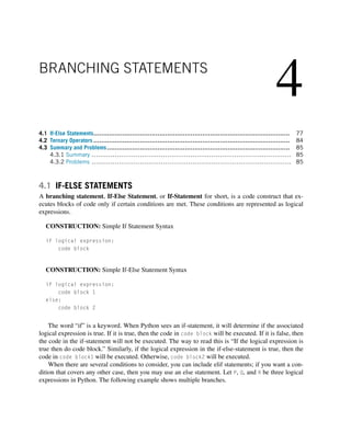
![78 CHAPTER 4 BRANCHING STATEMENTS
Note! Python gives the same level of indentation to every line of code within a conditional state-
ment.
CONSTRUCTION: Extended If-Else Statement Syntax
if logical expression P:
code block 1
elif logical expression Q:
code block 2
elif logical expression R:
code block 3
else:
code block 4
In the previous code, Python will first check if P is true. If P is true, then code block 1 will be
executed, and then the if-statement will end. In other words, Python will not check the rest of the
statements once it reaches a true statement. If P is false, then Python will check if Q is true. If Q is true,
then code block 2 will be executed, and the if-statement will end. If it is false, then R will be executed,
and so forth. If P, Q, and R are all false, then code block 4 will be executed. You can have any number
of elif statements (or none) as long as there is at least one if-statement (the first statement). You
do not need an else statement, but you can have, at most, one else statement. The logical expressions
after the if and elif (i.e., such as P, Q, and R) will be referred to as conditional statements.
TRY IT! Write a function my_thermo_stat(temp, desired_temp). The return value of the func-
tion should be the string Heat if temp is less than desired_temp minus 5 degrees, AC if temp
is more than the desired_temp plus 5, and off otherwise.
In [1]: def my_thermo_stat(temp, desired_temp):
Changes the status of the thermostat based on
temperature and desired temperature
author
date
:type temp: Int
:type desiredTemp: Int
:rtype: String
if temp desired_temp - 5:
status = Heat
elif temp desired_temp + 5:
status = AC
else:](https://image.slidesharecdn.com/pythonprogrammingandnumericalmethodsaguideforengineersand-231017183839-0fbc5295/85/Python_Programming_and_Numerical_Methods_A_Guide_for_Engineers_and-pdf-92-320.jpg)
![4.1 IF-ELSE STATEMENTS 79
status = off
return status
In [2]: status = my_thermo_stat(65,75)
print(status)
Heat
In [3]: status = my_thermo_stat(75,65)
print(status)
AC
In [4]: status = my_thermo_stat(65,63)
print(status)
off
EXAMPLE: What will be the value of y after the following script is executed?
In [5]: x = 3
if x 1:
y = 2
elif x 2:
y = 4
else:
y = 0
print(y)
2
We can also insert more complicated conditional statements using logical operators.
EXAMPLE: What will be the value of y after the following code is executed?
In [6]: x = 3
if x 1 and x 2:
y = 2
elif x 2 and x 4:
y = 4
else:
y = 0
print(y)](https://image.slidesharecdn.com/pythonprogrammingandnumericalmethodsaguideforengineersand-231017183839-0fbc5295/85/Python_Programming_and_Numerical_Methods_A_Guide_for_Engineers_and-pdf-93-320.jpg)
![80 CHAPTER 4 BRANCHING STATEMENTS
4
Note that if you want the logical statement a x b, this is considered as two conditional state-
ments, a x and x b. Python allows you to type a x b as well. For example,
In [7]: x = 3
if 1 x 2:
y = 2
elif 2 x 4:
y = 4
else:
y = 0
print(y)
4
A statement is called nested if it is entirely contained within another statement of the same type as
itself. For example, a nested if-statement is an if-statement that is entirely contained within a clause
of another if-statement.
EXAMPLE: Think about what will happen when the following code is executed. What are all
the possible outcomes based on the input values of x and y?
In [8]: def my_nested_branching(x,y):
Nested Branching Statement Example
author
date
:type x: Int
:type y: Int
:rtype: Int
if x 2:
if y 2:
out = x + y
else:
out = x - y
else:
if y 2:
out = x*y
else:](https://image.slidesharecdn.com/pythonprogrammingandnumericalmethodsaguideforengineersand-231017183839-0fbc5295/85/Python_Programming_and_Numerical_Methods_A_Guide_for_Engineers_and-pdf-94-320.jpg)
![4.1 IF-ELSE STATEMENTS 81
out = 0
return out
Note! As before, Python gives the same level of indentation to every line of code within a condi-
tional statement. The nested if-statement should be indented by an additional four white spaces.
You will get an IndentationError if the indentation is not correct, as we saw earlier when dis-
cussing how to define functions.
In [9]: import numpy as np
In [10]: all([1, 1, 0])
Out[10]: False
There are many logical functions that are designed to help you build branching statements. For exam-
ple, you can ask if a variable has a certain data type with function isinstance. There are also functions
that can tell you information about arrays of logicals like any, which computes to true if any element
in an array is true, and false otherwise, and all, which computes to true only if all the elements in an
array are true.
Sometimes you want to design your function to check the inputs of a function to ensure that your
function will be used properly. For example, the function my_adder in the previous chapter expects
doubles as input. If the user inputs a list or a string as one of the input variables, then the function
will throw an error or have unexpected results. To prevent this, you can put a check to tell the user
the function has not been used properly. This and other techniques for controlling errors are explored
further in Chapter 10. For the moment, you only need to know that we can use the raise statement
with a TypeError exception to stop a function’s execution and throw an error with a specific text.
EXAMPLE: Modify my_adder to throw out a warning if the user does not input numerical values.
Try your function for nonnumerical inputs to show that the check works. When a statement is too
long, we can use the “” symbol to break a line into multiple lines.
In [11]: def my_adder(a, b, c):
Calculate the sum of three numbers
author
date
# Check for erroneous input
if not (isinstance(a, (int, float))
or isinstance(b, (int, float))
or isinstance(c, (int, float))):](https://image.slidesharecdn.com/pythonprogrammingandnumericalmethodsaguideforengineersand-231017183839-0fbc5295/85/Python_Programming_and_Numerical_Methods_A_Guide_for_Engineers_and-pdf-95-320.jpg)
![82 CHAPTER 4 BRANCHING STATEMENTS
raise TypeError(Inputs must be numbers.)
# Return output
return a + b + c
In [12]: x = my_adder(1,2,3)
print(x)
6
In [13]: x = my_adder(1,2,3)
print(x)
------------------------------------------------------
TypeError Traceback (most recent call last)
ipython-input-13-c3e353c636b0 in module
---- 1 x = my_adder(1,2,3)
2 print(x)
ipython-input-11-0f3d29eecee0 in my_adder(a, b, c)
10 or isinstance(b, (int, float))
11 or isinstance(c, (int, float))):
--- 12 raise TypeError(Inputs must be numbers.)
13 # Return output
14 return a + b + c
TypeError: Inputs must be numbers.
There is a large variety of erroneous inputs that your function may encounter from users, and it is
unreasonable to expect that your function will catch them all. Therefore, unless otherwise stated, write
your functions assuming the functions will be used properly.
The remainder of the section gives a few more examples of branching statements.
TRY IT! Write a function called is_odd that returns odd if the input is an odd number and
even if it is even. You can assume that input will be a positive integer.
In [14]: def is_odd(number):
function returns odd if the input is odd,](https://image.slidesharecdn.com/pythonprogrammingandnumericalmethodsaguideforengineersand-231017183839-0fbc5295/85/Python_Programming_and_Numerical_Methods_A_Guide_for_Engineers_and-pdf-96-320.jpg)
![4.1 IF-ELSE STATEMENTS 83
even otherwise
author
date
:type number: Int
:rtype: String
# use modulo to check if the input divisible by 2
if number % 2 == 0:
# if divisible by 2, then input is not odd
return even
else:
return odd
In [15]: is_odd(11)
Out[15]: odd
In [16]: is_odd(2)
Out[16]: even
TRY IT! Write a function called my_circ_calc that takes a numerical number, r, and a string,
calc, as input arguments. You may assume that r is positive, and that calc is either the string
area or circumference. The function my_circ_calc should compute the area of a circle with
radius, r, if the string calc is the area, and the circumference of a circle with radius, r, if calc
is the circumference.
In [17]: np.pi
Out[17]: 3.141592653589793
In [18]: def my_circ_calc(r, calc):
Calculate various circle measurements
author
date
:type r: Int or Float
:type calc: String
:rtype: Int or Float
if calc == area:
return np.pi*r**2](https://image.slidesharecdn.com/pythonprogrammingandnumericalmethodsaguideforengineersand-231017183839-0fbc5295/85/Python_Programming_and_Numerical_Methods_A_Guide_for_Engineers_and-pdf-97-320.jpg)
![84 CHAPTER 4 BRANCHING STATEMENTS
elif calc == circumference:
return 2*np.pi*r
In [19]: my_circ_calc(2.5, area)
Out[19]: 19.634954084936208
In [20]: my_circ_calc(3, circumference)
Out[20]: 18.84955592153876
Note! The function here is not limited to a single value input but can be executed using NumPy
arrays as well (i.e., the same operation will apply on each item of the array). See the following
example where we calculate the circumferences for radius as [2, 3, 4] using a NumPy array.
In [21]: my_circ_calc(np.array([2, 3, 4]), circumference)
Out[21]: array([12.56637061, 18.84955592, 25.13274123])
4.2 TERNARY OPERATORS
Most programming languages have ternary operators, which are usually known as conditional ex-
pressions, that provide a mechanism using a one-line code to evaluate the first expression if the
condition is true; otherwise, it evaluates the second expression. To implement the ternary operator
in Python, use the construction presented below:
CONSTRUCTION: ternary operator in Python
expression_if_true if condition else expression_if_false
EXAMPLE: Ternary operator
In [1]: is_student = True
person = student if is_student else not student
print(person)
student
From the above example, we can see this one-line code is equivalent to the following block of
codes.](https://image.slidesharecdn.com/pythonprogrammingandnumericalmethodsaguideforengineersand-231017183839-0fbc5295/85/Python_Programming_and_Numerical_Methods_A_Guide_for_Engineers_and-pdf-98-320.jpg)
![4.3 SUMMARY AND PROBLEMS 85
In [2]: is_student = True
if is_student:
person = student
else:
person = not student
print(person)
student
Ternary operators provide a simple way for branching and can make our codes concise. In the next
chapter, we introduce its role in list comprehensions, and will prove it is useful.
4.3 SUMMARY AND PROBLEMS
4.3.1 SUMMARY
1. Branching (if-else) statements allow functions to take different actions under different circum-
stances.
2. Ternary operators allow single line branching statements.
4.3.2 PROBLEMS
1. Write a function my_tip_calc(bill, party) where bill is the total cost of a meal and party is
the number of people in the group. The tip should be calculated as 15% for a party strictly less than
six people, 18% for a party strictly less than eight, 20% for a party less than 11, and 25% for a party
11 or more. A couple of test cases are given below.
In [ ]: def my_tip_calc(bill, party):
# write your function code here
return tips
In [ ]: # t = 16.3935
t = my_tip_calc(109.29,3)
print(t)
In [ ]: # t = 19.6722
t = my_tip_calc(109.29,7)
print(t)
In [ ]: # t = 21.8580
t = my_tip_calc(109.29,9)
print(t)
In [ ]: # t = 27.3225
t = my_tip_calc(109.29,12)
print(t)](https://image.slidesharecdn.com/pythonprogrammingandnumericalmethodsaguideforengineersand-231017183839-0fbc5295/85/Python_Programming_and_Numerical_Methods_A_Guide_for_Engineers_and-pdf-99-320.jpg)
![86 CHAPTER 4 BRANCHING STATEMENTS
2. Write a function my_mult_operation(a,b,operation). The input argument, operation, is a string
that is either plus, minus, mult, div, or pow, and the function should compute: a + b,
a − b, a ∗ b, a/b, and ab for the respective values for operation. A couple of test cases are given
below.
In [ ]: def my_mult_operation(a,b,operation):
# write your function code here
return out
In [ ]: x = np.array([1,2,3,4])
y = np.array([2,3,4,5])
In [ ]: # Output: [3,5,7,9]
my_mult_operation(x,y,plus)
In [ ]: # Output: [-1,-1,-1,-1]
my_mult_operation(x,y,minus)
In [ ]: # Output: [2,6,12,20]
my_mult_operation(x,y,mult)
In [ ]: # Output: [0.5,0.66666667,0.75,0.8]
my_mult_operation(x,y,div)
In [ ]: # Output: [1,8,81,1024]
my_mult_operation(x,y,pow)
3. Consider a triangle with vertices at (0,0), (1,0), and (0,1). Write a function with the name
my_inside_triangle(x,y) where the output is the string outside if the point (x,y) is outside
of the triangle, border if the point is exactly on the border of the triangle, and inside if the
point is on the inside of the triangle.
In [ ]: def my_inside_triangle(x,y):
# write your function code here
return position
In [ ]: # Output: border
my_inside_triangle(.5,.5)
In [ ]: # Output: inside
my_inside_triangle(.25,.25)
In [ ]: # Output: outside
my_inside_triangle(5,5)
4. Write a function my_make_size10(x) where x is an array, and output is the first 10 elements of x if
x has more than 10 elements, and output is the array x padded with enough zeros to make it length
10 if x has less than 10 elements.](https://image.slidesharecdn.com/pythonprogrammingandnumericalmethodsaguideforengineersand-231017183839-0fbc5295/85/Python_Programming_and_Numerical_Methods_A_Guide_for_Engineers_and-pdf-100-320.jpg)
![4.3 SUMMARY AND PROBLEMS 87
In [ ]: def my_make_size10(x):
# write your function code here
return size10
In [ ]: # Output: [1,2,0,0,0,0,0,0,0,0]
my_make_size10(range(1,2))
In [ ]: # Output: [1,2,3,4,5,6,7,8,9,10]
my_make_size10(range(1,15))
In [ ]: # Output: [3,6,13,4,0,0,0,0,0,0]
my_make_size10(5,5)
5. Can you write my_make_size10 without using if-statements (i.e., using only logical and array oper-
ations)?
6. Write a function my_letter_grader(percent) where the grade is the string A+ if percent is
greater than 97, A if percent is greater than 93, A- if percent is greater than 90, B+ if
percent is greater than 87, B if percent is greater than 83, B- if percent is greater than 80,
C+ if percent is greater than 77, C if percent is greater than 73, C- if percent is greater than
70, D+ if percent is greater than 67, D if percent is greater than 63, D- if percent is greater
than 60, and F for any percent less than 60. Grades exactly on the division should be included in
the higher grade category.
In [ ]: def my_letter_grader(percent):
# write your function code here
return grade
In [ ]: # Output: A+
my_letter_grader(97)
In [ ]: # Output: B
my_letter_grader(84)
7. Most engineering systems have a built-in redundancy. That is, an engineering system has fail-safes
incorporated into the design to accomplish its purpose. Consider a nuclear reactor whose tempera-
ture is monitored by three sensors. An alarm should go off if any two of the sensor readings disagree.
Write a function my_nuke_alarm(s1,s2,s3) where s1, s2, and s3 are the temperature readings for
sensor 1, sensor 2, and sensor 3, respectively. The output should be the string alarm! if any two
of the temperature readings disagree by strictly more than 10 degrees and normal otherwise.
In [ ]: def my_nuke_alarm(s1,s2,s3):
# write your function code here
return response
In [ ]: #Output: normal
my_nuke_alarm(94,96,90)](https://image.slidesharecdn.com/pythonprogrammingandnumericalmethodsaguideforengineersand-231017183839-0fbc5295/85/Python_Programming_and_Numerical_Methods_A_Guide_for_Engineers_and-pdf-101-320.jpg)
![88 CHAPTER 4 BRANCHING STATEMENTS
In [ ]: #Output: alarm!
my_nuke_alarm(94,96,80)
In [ ]: #Output: normal
my_nuke_alarm(100,96,90)
8. Let Q(x) be the quadratic equation Q(x) = ax2 + bx + c for some scalar values a, b, and c. A root
of Q(x) is an r such that Q(r) = 0. The two roots of a quadratic equation can be described by the
quadratic formula, which is
r =
−b ±
√
b2 − 4ac
2a
.
A quadratic equation has either two real roots (i.e., b2 4ac), two imaginary roots (i.e., b2 4ac),
or one root r = − b
2a .
Write a function my_n_roots(a,b,c), where a, b, and c are the coefficients of the quadratic Q(x).
The function should return two values: n_roots and r. Also n_roots is 2 if Q has two real roots, 1
if Q has one root, −2 if Q has two imaginary roots, and r is an array containing the roots of Q.
In [ ]: def my_n_roots(a,b,c):
# write your function code here
return n_roots, r
In [ ]: # Output: n_roots = 2, r = [3, -3]
n_roots, r = my_n_roots(1,0,-9)
print(n_roots, r)
In [ ]: # Output: n_roots = -2,
# r = [-0.6667 + 1.1055i, -0.6667 - 1.1055i]
my_n_roots(3,4,5)
In [ ]: # Output: n_roots = 1, r = [1]
my_n_roots(2,4,2)
9. Write a function my_split_function(f,g,a,b,x), where f and g are function objects f(x) and
g(x), respectively. The output should be f(x) if x ≤ a, g(x) if x ≥ b, and 0 otherwise. Assume
that b a.
In [ ]: def my_split_function(f,g,a,b,x):
if x=a:
return f(x)
elif x=b:
return g(x)
else:
return 0
In [ ]: # Output: 2.713
my_split_function(np.exp,np.sin,2,4,1)](https://image.slidesharecdn.com/pythonprogrammingandnumericalmethodsaguideforengineersand-231017183839-0fbc5295/85/Python_Programming_and_Numerical_Methods_A_Guide_for_Engineers_and-pdf-102-320.jpg)
![4.3 SUMMARY AND PROBLEMS 89
In [ ]: # Output: 0
my_split_function(np.exp,np.sin,2,4,3)
In [ ]: # Output: -0.9589
my_split_function(np.exp,np.sin,2,4,5)](https://image.slidesharecdn.com/pythonprogrammingandnumericalmethodsaguideforengineersand-231017183839-0fbc5295/85/Python_Programming_and_Numerical_Methods_A_Guide_for_Engineers_and-pdf-103-320.jpg)
![5
ITERATION
5.1 For-Loops ............................................................................................................... 91
5.2 While Loops............................................................................................................ 97
5.3 Comprehensions....................................................................................................... 100
5.3.1 List Comprehension................................................................................... 100
5.3.2 Dictionary Comprehension ........................................................................... 101
5.4 Summary and Problems.............................................................................................. 101
5.4.1 Summary ............................................................................................... 101
5.4.2 Problems ............................................................................................... 101
5.1 FOR-LOOPS
A for-loop is a set of instructions that is repeated, or iterated, for every value in a sequence. Sometimes
for-loops are referred to as definite loops because they have a predefined beginning and end as bounded
by the sequence.
The general syntax of a for-loop block is as follows.
CONSTRUCTION: For-loop
for looping variable in sequence:
code block
A for-loop assigns the looping variable to the first element of the sequence. It executes everything
in the code block. Then it assigns the looping variable to the next element of the sequence and executes
the code block again. It continues until there are no more elements in the sequence to assign.
TRY IT! What is the sum of every integer from 1 to 3?
In [1]: n = 0
for i in range(1, 4):
n = n + i
print(n)](https://image.slidesharecdn.com/pythonprogrammingandnumericalmethodsaguideforengineersand-231017183839-0fbc5295/85/Python_Programming_and_Numerical_Methods_A_Guide_for_Engineers_and-pdf-104-320.jpg)
![92 CHAPTER 5 ITERATION
6
WHAT IS HAPPENING?
0. First, the function range(1, 4) generates a sequence of numbers that begin at 1 and end at
3. Check the description of the function range and get familiar with how to use it. In a very
simple form, it is range(start, stop, step), and the step is optional with 1 as the default.
1. The variable n is assigned the value 0.
2. The variable i is assigned the value 1.
3. The variable n is assigned the value n + i (0 + 1 = 1).
4. The variable i is assigned the value 2.
5. The variable n is assigned the value n + i (1 + 2 = 3).
6. The variable i is assigned the value 3.
7. The variable n is assigned the value n + i (3 + 3 = 6).
8. With no more values to assign in the list, the for-loop is terminated with n = 6.
Below are several more examples to give you a sense of how for-loops work. Other examples of
sequences that we can iterate over include the elements of a tuple, the characters in a string, and other
sequential data types.
EXAMPLE: Print all the characters in the string banana.
In [2]: for c in banana:
print(c)
b
a
n
a
n
a
Alternatively, you can use the index to get each character, but it is not as concise as the previous
example. Recall that the length of a string can be determined by using the len function, and we can
ignore the start by only giving one number as the stop.
In [3]: s = banana
for i in range(len(s)):
print(s[i])
b
a
n
a](https://image.slidesharecdn.com/pythonprogrammingandnumericalmethodsaguideforengineersand-231017183839-0fbc5295/85/Python_Programming_and_Numerical_Methods_A_Guide_for_Engineers_and-pdf-105-320.jpg)
![5.1 FOR-LOOPS 93
n
a
EXAMPLE: Given a list of integers, a, add all the elements of a.
In [4]: s = 0
a = [2, 3, 1, 3, 3]
for i in a:
s += i # note this is equivalent to s = s + i
print(s)
12
The Python function sum has already been written to handle the previous example. What if you
want to add the even indices numbers only? What change(s) would you make to the previous for-loop
block to handle this restriction?
In [5]: s = 0
for i in range(0, len(a), 2):
s += a[i]
print(s)
6
NOTE! We use step as 2 in the range function to get the even indexes for list a. A commonly
used Python shortcut is the operator +=. In Python and many other programming languages, a
statement like i += 1 is equivalent to i = i + 1 and is the same for other operators as -=, *=, /=.
EXAMPLE: Define a dictionary and loop through all the keys and values.
In [6]: dict_a = {One:1, Two:2, Three:3}
for key in dict_a.keys():
print(key, dict_a[key])
One 1
Two 2
Three 3
In the above example, we used the method keys first to retrieve all keys. Next, we used the key to get
access the value. Alternatively, we can use the items method in a dictionary, which returns an object
containing a list of key and value pairs in tuple. We can assign them simultaneously to two variables
(tuple assignment); see the example below.](https://image.slidesharecdn.com/pythonprogrammingandnumericalmethodsaguideforengineersand-231017183839-0fbc5295/85/Python_Programming_and_Numerical_Methods_A_Guide_for_Engineers_and-pdf-106-320.jpg)
![94 CHAPTER 5 ITERATION
In [7]: for key, value in dict_a.items():
print(key, value)
One 1
Two 2
Three 3
Note that we can assign two different looping variables at the same time. There are other cases where
we can assign tasks simultaneously. For example, if we have two lists with same length and we want
to loop through them simultaneously, we use the zip function. See the example below. This function
aggregates elements from two iterables and returns an iterator of tuples, where the ith tuple element
contains the ith element of each of the iterables.
In [8]: a = [One, Two, Three]
b = [1, 2, 3]
for i, j in zip(a, b):
print(i, j)
One 1
Two 2
Three 3
EXAMPLE: Let the function have_digits have a string as the input. The output out should take
the value 1 if the string contains digits, and 0 otherwise. You can apply the isdigit method of
the string to check if the character is a digit.
In [9]: def have_digits(s):
out = 0
# loop through the string
for c in s:
# check if the character is a digit
if c.isdigit():
out = 1
break
return out
In [10]: out = have_digits(only4you)
print(out)](https://image.slidesharecdn.com/pythonprogrammingandnumericalmethodsaguideforengineersand-231017183839-0fbc5295/85/Python_Programming_and_Numerical_Methods_A_Guide_for_Engineers_and-pdf-107-320.jpg)
![5.1 FOR-LOOPS 95
1
In [11]: out = have_digits(only for you)
print(out)
0
The first step in the function have_digits assumes that there are no digits in the string s (i.e., the
output is 0 or False).
Notice the new keyword break. If executed, the break keyword immediately stops the most imme-
diate for-loop that contains it; that is, if it is contained in a nested for-loop, then it will only stop
the innermost for-loop. In this particular case, the break command is executed if we ever find a digit in
the string. The code will still function properly without this statement, but since the task is to find out
if there are any digits in s, we do not have to keep looking if we find one. Similarly, if a human was
given the same task for a long string of characters, that person would not continue looking for digits
if he or she already found one. Break statements are used when anything happens in a for-loop that
would make you want to stop the run early. A less intrusive command is the keyword continue, which
skips the remaining code in the current iteration of the for-loop, and continues on to the next element
of the looping array. See the following example where we use the keyword continue to skip the print
function to print 2:
In [12]: for i in range(5):
if i == 2:
continue
print(i)
0
1
3
4
EXAMPLE: Let the function my_dist_2_points(xy_points, xy) where the input argument
xy_points is a list of x–y coordinates of a point in Euclidean space, xy is a list that contain an
x–y coordinate, and the output d is a list containing the distances from xy to the points contained
in each row of xy_points.
In [13]: import math
def my_dist_2_points(xy_points, xy):
Returns an array of distances between xy and the](https://image.slidesharecdn.com/pythonprogrammingandnumericalmethodsaguideforengineersand-231017183839-0fbc5295/85/Python_Programming_and_Numerical_Methods_A_Guide_for_Engineers_and-pdf-108-320.jpg)
![96 CHAPTER 5 ITERATION
points contained in the rows of xy_points
author
date
d = []
for xy_point in xy_points:
dist = math.sqrt((xy_point[0]-xy[0])**2+(xy_point[1]-xy[1])**2)
d.append(dist)
return d
In [14]: xy_points = [[3,2], [2, 3], [2, 2]]
xy = [1, 2]
my_dist_2_points(xy_points, xy)
Out[14]: [2.0, 1.4142135623730951, 1.0]
Just like if-statements, for-loops can be nested.
EXAMPLE: Let x be a two-dimensional array, [5 6;7 8]. Use a nested for-loop to sum all the
elements in x.
In [15]: x = np.array([[5, 6], [7, 8]])
n, m = x.shape
s = 0
for i in range(n):
for j in range(m):
s += x[i, j]
print(s)
26
WHAT IS HAPPENING?
1. s, representing the running total sum, is set to 0.
2. The outer for-loop begins with looping variable, i, set to 0.
3. Inner for-loop begins with looping variable, j, set to 0.
4. s is incremented by x[i,j] = x[0,0] = 5. So s = 5.
5. Inner for-loop sets j = 1.
6. s is incremented by x[i,j] = x[0,1] = 6; therefore, s = 11.
7. Inner for-loop terminates.](https://image.slidesharecdn.com/pythonprogrammingandnumericalmethodsaguideforengineersand-231017183839-0fbc5295/85/Python_Programming_and_Numerical_Methods_A_Guide_for_Engineers_and-pdf-109-320.jpg)
![5.2 WHILE LOOPS 97
8. Outer for-loop sets i = 1.
9. Inner for-loop begins with looping variable, j, set to 0.
10. s is incremented by x[i,j] = x[1,0] = 7; therefore, s = 18.
11. Inner for-loop sets j = 1.
12. s is incremented by x[i,j] = x[1,1] = 8. So s = 26.
13. Inner for-loop terminates.
14. Outer for-loop terminates with s = 26.
WARNING! Although it is possible to do so, do not try to change the looping variable inside of
the for-loop. It will make your code very complicated and will likely result in errors.
5.2 WHILE LOOPS
A while-loop or indefinite loop is a set of instructions that is repeated as long as the associated logical
expression is true. The following is the abstract syntax of a while-loop block.
CONSTRUCTION: While Loop
while logical expression:
# Code block to be repeated until logical statement is false
code block
When Python reaches a while-loop block, it first determines if the logical expression of the while-
loop is true or false. If the expression is true, the code block will be executed. After it is executed, the
program returns to the logical expression at the beginning of the while statement. If it is false, then
the while-loop will terminate.
TRY IT! Determine the number of times 8 can be divided by 2 until the result is less than 1.
In [1]: i = 0
n = 8
while n = 1:
n /= 2
i += 1
print(fn = {n}, i = {i})
n = 0.5, i = 4](https://image.slidesharecdn.com/pythonprogrammingandnumericalmethodsaguideforengineersand-231017183839-0fbc5295/85/Python_Programming_and_Numerical_Methods_A_Guide_for_Engineers_and-pdf-110-320.jpg)
![98 CHAPTER 5 ITERATION
WHAT IS HAPPENING?
1. First the variable i (running count of divisions of n by 2) is set to 0.
2. n is set to 8 and represents the current value we are dividing by 2.
3. The while-loop begins.
4. Python evaluates expression n ≥ 1 or 8 ≥ 1, which is true; therefore, the code block is exe-
cuted.
5. n is assigned n/2 = 8/2 = 4.
6. i is incremented to 1.
7. Python evaluates expression n ≥ 1 or 4 ≥ 1, which is true; therefore, the code block is exe-
cuted.
8. n is assigned n/2 = 4/2 = 2.
9. i is incremented to 2.
10. Python evaluates expression n ≥ 1 or 2 ≥ 1, which is true; therefore, the code block is exe-
cuted.
11. n is assigned n/2 = 2/2 = 1.
12. i is incremented to 3.
13. Python evaluates expression n ≥ 1 or 1 ≥ 1, which is true; therefore, the code block is exe-
cuted.
14. n is assigned n/2 = 1/2 = 0.5.
15. i is incremented to 4.
16. Python evaluates expression n ≥ 1 or 0.5 ≥ 1, which is false; therefore, the while-loop ends
with i = 4.
You may ask, “What if the logical expression is true and never changes?”; an excellent question.
If the logical expression is true and nothing in the while-loop code changes the expression, then the
result is known as an infinite loop. Infinite loops run forever, or until your computer breaks, or runs
out of memory.
EXAMPLE: Write a while-loop that causes an infinite loop.
In [ ]: n = 0
while n -1:
n += 1
Since n will always be bigger than -1 no matter how many times the loop is run, this code will never
end.
You can terminate the infinite while loop manually by pressing the interrupt the kernel – the
black square button in the tool bar above shown in Fig. 5.1, or the drop down menu - Kernel - In-
terrupt in the notebook. Or if you are using the Python shell, press cmd + c on Mac or Ctrl + c on
PC.
Can you change a single character so that the while-loop will run at least once but will not infinite
loop?](https://image.slidesharecdn.com/pythonprogrammingandnumericalmethodsaguideforengineersand-231017183839-0fbc5295/85/Python_Programming_and_Numerical_Methods_A_Guide_for_Engineers_and-pdf-111-320.jpg)
![5.2 WHILE LOOPS 99
FIGURE 5.1
Interrupt the kernel by pressing the little square.
Infinite loops are not always easy to spot. Consider the next two examples: one performs infinite
loops and one does not. Can you determine which is which? As your code becomes more complicated,
it will become harder to detect.
EXAMPLE: Which while-loop causes an infinite loop?
In [ ]: # Example 1
n = 1
while n 0:
n /= 2
In [ ]: # Example 2
n = 2
while n 0:
if n % 2 == 0:
n += 1
else:
n -= 1
Answer: The first example will not infinite loop because eventually n will be so small that
Python cannot tell the difference between n and 0. This will be discussed in more detail in Chap-
ter 9. The second example will infinite loop because n will oscillate between 2 and 3 indefinitely.
Now we know two types of loops: for-loops and while-loops. In some cases, either are appropri-
ate, but sometimes one is better suited for the task than the other. In general, use for-loops when the
number of iterations to be performed is well-defined; use while-loops statements when the number of
iterations to be performed is indefinite or not well known.](https://image.slidesharecdn.com/pythonprogrammingandnumericalmethodsaguideforengineersand-231017183839-0fbc5295/85/Python_Programming_and_Numerical_Methods_A_Guide_for_Engineers_and-pdf-112-320.jpg)
![100 CHAPTER 5 ITERATION
5.3 COMPREHENSIONS
In Python, there are other ways to do iterations; list, dictionary, and set comprehensions are very
popular ways. Once you familiarize yourself with them, you will find yourself using them a lot. Com-
prehensions allow sequences to be created from other sequences using very compact syntax. Let us
first look at the list comprehension.
5.3.1 LIST COMPREHENSION
CONSTRUCTION: List comprehension
[Output Input_sequence Conditions]
EXAMPLE: If x = range(5), square each number in x, and store it in a list y.
If we do not use list comprehension, the code will look something like this:
In [1]: x = range(5)
y = []
for i in x:
y.append(i**2)
print(y)
[0, 1, 4, 9, 16]
Using the list comprehension, we can write just one line.
In [2]: y = [i**2 for i in x]
print(y)
[0, 1, 4, 9, 16]
In addition, we can also include conditions in the list comprehension. For example, if we just want
to store the even numbers in the above example, we just add a condition in the list comprehension.
In [3]: y = [i**2 for i in x if i%2 == 0]
print(y)
[0, 4, 16]
If we have two nested levels for loops, we can also use the list comprehensions. For example, we
have the following two levels for loops that we can perform using the list comprehension.](https://image.slidesharecdn.com/pythonprogrammingandnumericalmethodsaguideforengineersand-231017183839-0fbc5295/85/Python_Programming_and_Numerical_Methods_A_Guide_for_Engineers_and-pdf-113-320.jpg)
![5.4 SUMMARY AND PROBLEMS 101
In [4]: y = []
for i in range(5):
for j in range(2):
y.append(i + j)
print(y)
[0, 1, 1, 2, 2, 3, 3, 4, 4, 5]
In [5]: y = [i + j for i in range(5) for j in range(2)]
print(y)
[0, 1, 1, 2, 2, 3, 3, 4, 4, 5]
5.3.2 DICTIONARY COMPREHENSION
Similarly, we can do the dictionary comprehension as well. See the following example.
In [6]: x = {a: 1, b: 2, c: 3}
{key:v**3 for (key, v) in x.items()}
Out[6]: {a: 1, b: 8, c: 27}
Performing set comprehension is also possible in Python, but will not be explored here. This is a
task that you should explore on your own.
5.4 SUMMARY AND PROBLEMS
5.4.1 SUMMARY
1. Loops provide a mechanism for a code to perform repetitive tasks, that is, iteration.
2. There are two kinds of loops: for-loops and while-loops.
3. Loops are important for constructing iterative solutions to problems.
5.4.2 PROBLEMS
1. What will the value of y be after the following code is executed?
In [ ]: y = 0
for i in range(1000):
for j in range(1000):
if i == j:
y += 1
2. Write a function my_max(x) to return the maximum (largest) value in x. Do not use the built-in
Python function max.](https://image.slidesharecdn.com/pythonprogrammingandnumericalmethodsaguideforengineersand-231017183839-0fbc5295/85/Python_Programming_and_Numerical_Methods_A_Guide_for_Engineers_and-pdf-114-320.jpg)
![102 CHAPTER 5 ITERATION
3. Write a function my_n_max(x, n) to return a list consisting of the n largest elements of x. You may
use Python’s max function. You may also assume that x is a one-dimensional list with no duplicate
entries, and that n is a strictly positive integer smaller than the length of x
In [ ]: x = [7, 9, 10, 5, 8, 3, 4, 6, 2, 1]
def my_n_max(x, n):
# write your function code here
return out
In [ ]: # Output = [10, 9, 8]
out = my_n_max(x, n)
print(out)
4. Let m be a matrix of positive integers. Write a function my_trig_odd_even(m) to return an array q,
where q[i, j] = sin(m[i, j]) if m[i, j] is even, and q[i, j] = cos(m[i, j]) if m[i, j] is
odd.
5. Let P be an m × p array and Q be a p × n array. As you will find later in this book, M = P ×
Q is defined as M[i,j] =
p
k=1 P[i,k] · Q[k,j]. Write a function my_mat_mult(P, Q) that uses
for-loops to compute M, the matrix product of P * Q. Hint: You may need up to three nested
for-loops. Do not use the function np.dot.
In [ ]: import numpy as np
def my_mat_mult(P, Q):
# write your function code here
return M
In [ ]: # Output:
# array([[3., 3., 3.],
# [3., 3., 3.],
# [3., 3., 3.]])
P = np.ones((3, 3))
my_mat_mult(P, P)
In [ ]: # Output:
# array([[30, 30, 30],
# [70, 70, 70]])
P = np.array([[1, 2, 3, 4], [5, 6, 7, 8]])
Q = np.array([[1, 1, 1], [2, 2, 2], [3, 3, 3], [4, 4, 4]])
my_mat_mult(P, Q)](https://image.slidesharecdn.com/pythonprogrammingandnumericalmethodsaguideforengineersand-231017183839-0fbc5295/85/Python_Programming_and_Numerical_Methods_A_Guide_for_Engineers_and-pdf-115-320.jpg)
![5.4 SUMMARY AND PROBLEMS 103
6. The interest i on a principle, P0, is a payment for allowing the bank to use your money. Compound
interest is accumulated according to the formula Pn = (1 + i)Pn−1, where n is the compounding
period, usually in months or years. Write a function my_saving_plan(P0, i, goal) where the
output is the number of years it will take P0 to become goal at i% interest compounded annually.
In [ ]: def my_saving_plan(P0, i, goal):
# write your function code here
return years
In [ ]: # Output: 15
my_saving_plan(1000, 0.05, 2000)
In [ ]: # Output: 11
my_saving_plan(1000, 0.07, 2000)
In [ ]: # Output: 21
my_saving_plan(500, 0.07, 2000)
7. Write a function with my_find(M) where the output is a list of indices i and where M[i] is 1. You
may assume that M is a list of only ones and zeros. Do not use the built-in Python function find.
In [ ]: # Output: [0, 2, 3]
M = [1, 0, 1, 1, 0]
my_find(M)
8. Assume you are rolling two six-sided dice, with each side having an equal chance of occurring.
Write a function my_monopoly_dice() where the output is the sum of the values of the two dice
thrown but with the following extra rule: if the two dice rolls are the same, then another roll is
made, and the new sum added to the running total. For example, if the two dice show 3 and 4, then
the running total should be 7. If the two dice show 1 and 1, then the running total should be 2 plus
the total of another throw. Rolls stop when the dice rolls are different.
9. A number is prime if it is divisible without remainder only by itself and 1. The number 1 is not
a prime. Write a function my_is_prime(n) where the output is 1 if n is prime and 0 is otherwise.
Assume that n is a strictly positive integer.
10. Write a function my_n_primes(n) where prime is a list of the first n primes. Assume that n is a
strictly positive integer.
11. Write a function my_n_fib_primes(n) where the output fib_primes is a list of the first n numbers
that are both a Fibonacci number and a prime. Note that 1 is not prime. Hint: Do not use the
recursive implementation of Fibonacci numbers. A function to compute Fibonacci numbers is
presented in Section 6.1. You may use the code freely.
In [ ]: def my_n_fib_primes(n):
# write your function code here
return fib_primes](https://image.slidesharecdn.com/pythonprogrammingandnumericalmethodsaguideforengineersand-231017183839-0fbc5295/85/Python_Programming_and_Numerical_Methods_A_Guide_for_Engineers_and-pdf-116-320.jpg)
![104 CHAPTER 5 ITERATION
In [ ]: # Output: [3, 5, 13, 89, 233, 1597, 28657, 514229]
my_n_fib_primes(3)
In [ ]: # Output: [3, 5, 13]
my_n_fib_primes(8)
12. Write a function my_trig_odd_even(M) where the output Q[i,j] = sin(π/M[i,j]) if M[i,j] is
odd, and Q[i,j] = cos(π/M[i,j]) if M[i,j] is even. Assume that M is a two-dimensional array
of strictly positive integers.
In [ ]: def my_trig_odd_even(M):
# write your function code here
return Q
In [ ]: # Output: [[0.8660, 0.7071], [0.8660, 0.4339]]
M = [[3, 4], [6, 7]]
my_trig_odd_even(M)
13. Let C be a square connectivity array containing zeros and ones. Point i has a connection to point
j or i is connected to j if C[i,j] = 1. Note that connections in this context are one-directional,
meaning C[i,j] is not necessarily the same as C[j,i]. For example, think of a one-way street
from point A to point B. If A is connected to B, then B is not necessarily connected to A.
Write a function my_connectivity_mat_2_dict(C, names) where C is a connectivity array and
names is a list of strings that denote the name of a point. That is, names[i] is the name of the name
of the ith point.
The output variable node should be a dictionary with the key as the string in names, and value is
a vector containing the indices j, such that C[i,j] = 1. In other words, it is a list of points that
point i is connected to.
In [ ]: def my_connectivity_mat_2_dict(C, names):
# write your function code here
return node
In [ ]: C = [[0, 1, 0, 1], [1, 0, 0, 1], [0, 0, 0, 1], [1, 1, 1, 0]]
names = [Los Angeles, New York, Miami, Dallas]
In [ ]: # Output: node[Los Angeles] = [2, 4]
# node[New York] = [1, 4]
# node[Miami] = [4]
# node[Dallas] = [1, 2, 3]
node = my_connectivity_mat_2_dict(C, names)
14. Turn the list words of lower case characters to upper case using the list comprehension.
In [ ]: words = [test, data, analyze]](https://image.slidesharecdn.com/pythonprogrammingandnumericalmethodsaguideforengineersand-231017183839-0fbc5295/85/Python_Programming_and_Numerical_Methods_A_Guide_for_Engineers_and-pdf-117-320.jpg)
![6
RECURSION
6.1 Recursive Functions .................................................................................................. 105
6.2 Divide-and-Conquer................................................................................................... 110
6.2.1 Tower of Hanoi......................................................................................... 110
6.2.2 Quicksort ............................................................................................... 113
6.3 Summary and Problems.............................................................................................. 114
6.3.1 Summary ............................................................................................... 114
6.3.2 Problems ............................................................................................... 114
6.1 RECURSIVE FUNCTIONS
A recursive function is a function that makes calls to itself. It works like the loops we described before.
In some cases, however, it is preferable to use recursion than loops.
Every recursive function has two components: a base case and a recursive step. The base case is
usually the smallest input and has an easily verifiable solution. This is also the mechanism that stops
the function from calling itself forever. The recursive step is the set of all cases where a recursive
call, or a function call to itself, is made.
As an example, we will demonstrate how recursion can be used to define and compute the factorial
of an integer number. The factorial of an integer n is 1 × 2 × 3 × ··· × (n − 1) × n. The recursive
definition can be written as follows:
f (n) =
1 if n = 1,
n × f (n − 1) otherwise.
(6.1)
The base case is n = 1, which is trivial to compute: f (1) = 1. In the recursive step, n is multiplied
by the result of a recursive call to the factorial of n − 1.
TRY IT! Write the factorial function using recursion. Use your function to compute the factorial
of 3.
In [1]: def factorial(n):
Computes and returns the factorial of n,
a positive integer.
if n == 1: # Base case!](https://image.slidesharecdn.com/pythonprogrammingandnumericalmethodsaguideforengineersand-231017183839-0fbc5295/85/Python_Programming_and_Numerical_Methods_A_Guide_for_Engineers_and-pdf-118-320.jpg)
![106 CHAPTER 6 RECURSION
return 1
else: # Recursive step
return n * factorial(n - 1) # Recursive call
In [2]: factorial(3)
Out[2]: 6
WHAT IS HAPPENING? First recall that when Python executes a function, it creates a
workspace for the variables created in that function. Whenever a function calls another func-
tion, it will wait until that function returns an answer before continuing. In programming, this
workspace is called a stack. Similar to a stack of plates in our kitchen cabinet, elements in a stack
are added or removed from the top of the stack to the bottom, in a “last in, first out” order. For
example, in the np.sin(np.tan(x)), sin must wait for tan to return an answer before it can be
evaluated. Even though a recursive function makes calls to itself, the same rules apply.
1. A call is made to factorial(3), whereby a new workspace is opened to compute facto-
rial(3).
2. Input argument value 3 is compared to 1. Since they are not equal, the else statement is
executed.
3. 3*factorial(2) must be computed. A new workspace is opened to compute factorial(2).
4. Input argument value 2 is compared to 1. Since they are not equal, the else statement is
executed.
5. 2*factorial(1) must be computed. A new workspace is opened to compute factorial(1).
6. Input argument value 1 is compared to 1. Since they are equal, the if statement is executed.
7. The return variable is assigned the value 1. factorial(1) terminates with output 1.
8. 2*factorial(1) can be resolved to 2 × 1 = 2. The output is assigned the value 2. facto-
rial(2) terminates with output 2.
9. 3*factorial(2) can be resolved to 3 × 2 = 6. The output is assigned the value 6. Thus fac-
torial(3) terminates with output 6.
The order of recursive calls can be depicted by a recursion tree shown in Fig. 6.1 for factorial(3).
A recursion tree is a diagram of the function calls connected by numbered arrows to depict the order
in which the calls were made.
Fibonacci numbers were originally developed to model the idealized population growth of rabbits.
Since then, they have been found to be significant in any naturally occurring phenomena. The Fibonacci
numbers can be generated using the following recursive formula. Note that the recursive step contains
two recursive calls and that there are also two base cases (i.e., two cases that cause the recursion to
stop):
F(n) =
⎧
⎪
⎨
⎪
⎩
1 if n = 1,
1 if n = 2,
F(n − 1) + F(n − 2) otherwise.
(6.2)](https://image.slidesharecdn.com/pythonprogrammingandnumericalmethodsaguideforengineersand-231017183839-0fbc5295/85/Python_Programming_and_Numerical_Methods_A_Guide_for_Engineers_and-pdf-119-320.jpg)
![6.1 RECURSIVE FUNCTIONS 107
FIGURE 6.1
Recursion tree for factorial(3).
TRY IT! Write a recursive function for computing the nth Fibonacci number. Use your function
to compute the first five Fibonacci numbers. Draw the associated recursion tree.
In [3]: def fibonacci(n):
Computes and returns the Fibonacci of n,
a positive integer.
if n == 1: # first base case
return 1
elif n == 2: # second base case
return 1
else: # Recursive step
return fibonacci(n-1) + fibonacci(n-2)
In [4]: print(fibonacci(1))
print(fibonacci(2))
print(fibonacci(3))
print(fibonacci(4))
print(fibonacci(5))
1
1
2
3
5
As an exercise, consider the following modification to fibonacci, where the results of each recur-
sive call are displayed to the screen (see Fig. 6.2).](https://image.slidesharecdn.com/pythonprogrammingandnumericalmethodsaguideforengineersand-231017183839-0fbc5295/85/Python_Programming_and_Numerical_Methods_A_Guide_for_Engineers_and-pdf-120-320.jpg)
![108 CHAPTER 6 RECURSION
FIGURE 6.2
Recursion tree for factorial(5).
EXAMPLE: Write a function fib_disp(5) based on modification of the fibonacci function.
Can you determine the order in which the Fibonacci numbers will appear on the screen for
fib_disp(5)?
In [5]: def fib_disp(n):
Computes and returns the Fibonacci of n,
a positive integer.
if n == 1: # first base case
out = 1
print(out)
return out
elif n == 2: # second base case
out = 1
print(out)
return out
else: # Recursive step
out = fib_disp(n-1) + fib_disp(n-2)
print(out)
return out # Recursive call
1
1
2
1
3
1
1](https://image.slidesharecdn.com/pythonprogrammingandnumericalmethodsaguideforengineersand-231017183839-0fbc5295/85/Python_Programming_and_Numerical_Methods_A_Guide_for_Engineers_and-pdf-121-320.jpg)
![6.1 RECURSIVE FUNCTIONS 109
2
5
In [6]: fib_disp(5)
5
Note that the number of recursive calls becomes very large even for relatively small inputs for n. If
you do not agree, try to draw the recursion tree for fibonacci(10). If you try your unmodified function
for inputs around 35, you will experience significant computation times.
In [7]: fibonacci(35)
Out[7]: 9227465
There is an iterative method for computing the nth Fibonacci number that requires only one
workspace.
EXAMPLE: Iterative implementation for computing Fibonacci numbers.
In [8]: import numpy as np
def iter_fib(n):
fib = np.ones(n)
for i in range(2, n):
fib[i] = fib[i - 1] + fib[i - 2]
return fib
TRY IT! Compute the 25th Fibonacci number using iter_fib and fibonacci. Use the magic
command timeit to measure the run time for each. Note the large difference in running times.
In [9]: %timeit iter_fib(25)
7.22 µs ± 171 ns per loop (mean ± std. dev. of 7 runs, 100000 loops each)
In [10]: %timeit fibonacci(25)
16.7 ms ± 910 µs per loop (mean ± std. dev. of 7 runs, 100 loops each)
You can see in the previous example that the iterative version runs much faster than the recursive
counterpart. In general, iterative functions are faster than recursive functions performing the same task.
So why use recursive functions at all? There are some solution methods that have a naturally recursive](https://image.slidesharecdn.com/pythonprogrammingandnumericalmethodsaguideforengineersand-231017183839-0fbc5295/85/Python_Programming_and_Numerical_Methods_A_Guide_for_Engineers_and-pdf-122-320.jpg)
![110 CHAPTER 6 RECURSION
structure. In these cases, it is usually very hard to write a counterpart using loops. The primary value
of writing recursive functions is that they can usually be written much more compactly than iterative
functions. The cost of the improved compactness is added running time.
The relationship between the input arguments and the running time is discussed in more detail later
in the chapter on complexity.
TIP! Try to write functions iteratively whenever it is convenient to do so. Your functions will run
faster.
NOTE! When using a recursive call as shown above, we need to make sure that it can reach the
base case, otherwise, it enters infinite recursion. In Python, executing a recursive function on a
large output that cannot reach the base case will result in a “maximum recursion depth exceeded
error”. Try the following example to produce the RecursionError.
In []: factorial(5000)
We can work around the recursion limit using the sys module by setting a higher limit in Python.
If you run the following code, the error message won’t occur.
In []: import sys
sys.setrecursionlimit(10**5)
factorial(5000)
6.2 DIVIDE-AND-CONQUER
Divide-and-conquer is a useful strategy for solving difficult problems. Using divide-and-conquer,
difficult problems are solved from solutions to many similar easy problems. In this way, difficult prob-
lems are broken up so they are more manageable. This section will present two classical examples of
divide-and-conquer: the Tower of Hanoi Problem and the Quicksort algorithm.
6.2.1 TOWER OF HANOI
The Tower of Hanoi problem consists of three vertical rods (or towers) and N disks of different sizes,
each with a hole in the center so that the rod can slide through it. The original configuration of the disks
is that they are stacked on one of the towers in the order of descending size (i.e., the largest disc is on
the bottom). The goal of the problem is to move all the disks to a different rod while complying with
the following three rules:
1. Only one disk can be moved at a time.
2. Only the disk at the top of a stack may be moved.
3. A disk may not be placed on top of a smaller disk.](https://image.slidesharecdn.com/pythonprogrammingandnumericalmethodsaguideforengineersand-231017183839-0fbc5295/85/Python_Programming_and_Numerical_Methods_A_Guide_for_Engineers_and-pdf-123-320.jpg)
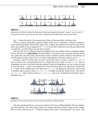
![112 CHAPTER 6 RECURSION
is a difficult task, so instead we make a recursive call that will make subsequent recursive calls, but
will, in the end, move the stack as desired. Then we move the bottom disk to the target “to_tower”.
Finally, we move the stack of size N − 1 to the target tower by making another recursive call.
TRY IT! Use the function my_towers to solve the Tower of Hanoi problem for N = 3. Verify the
solution is correct by inspection.
In [1]: def my_towers(N, from_tower, to_tower, alt_tower):
Displays the moves required to move a tower of size
N from the from_tower to the to_tower.
from_tower, to_tower and alt_tower are
either 1, 2, 3 referring to tower 1, 2, and 3.
if N != 0:
# recursive call that moves N-1 stack from
# starting tower to alternate tower
my_towers(N-1, from_tower, alt_tower, to_tower)
# display to screen movement of bottom disk from
# starting tower to final tower
print(Move disk %d from tower %d to tower %d.
%(N, from_tower, to_tower))
# recursive call that moves N-1 stack from
# alternate tower to final tower
my_towers(N-1, alt_tower, to_tower, from_tower)
In [2]: my_towers(3, 1, 3, 2)
Move disk 1 from tower 1 to tower 3.
Move disk 2 from tower 1 to tower 2.
Move disk 1 from tower 3 to tower 2.
Move disk 3 from tower 1 to tower 3.
Move disk 1 from tower 2 to tower 1.
Move disk 2 from tower 2 to tower 3.
Move disk 1 from tower 1 to tower 3.
By using divide-and-conquer, we have solved the Tower of Hanoi problem by making recursive
calls to the slightly smaller Tower of Hanoi problems that, in turn, make recursive calls to yet smaller
Tower of Hanoi problems. Together, the solutions form the solution to the whole problem. The actual
work done by a single function call is actually quite small: two recursive calls and moving one disk. In](https://image.slidesharecdn.com/pythonprogrammingandnumericalmethodsaguideforengineersand-231017183839-0fbc5295/85/Python_Programming_and_Numerical_Methods_A_Guide_for_Engineers_and-pdf-125-320.jpg)
![6.2 DIVIDE-AND-CONQUER 113
other words, a function call does very little work (moving a disk), and then passes the rest of the work
onto other calls, a skill you will find very useful throughout your engineering career.
6.2.2 QUICKSORT
A list of numbers, A, is sorted if the elements are arranged in ascending or descending order. Although
there are many ways of sorting a list, quicksort is a divide-and-conquer approach, which is a very fast
algorithm for sorting using a single processor (there are faster algorithms for multiple processors).
The quicksort algorithm starts with the observation that although sorting a list is hard, a comparison
is relatively easy. So instead of sorting a list, we separate the list by comparing to a pivot. At each
recursive call to quicksort, the input list is divided into three parts: elements that are smaller than the
pivot, elements that are equal to the pivot, and elements that are larger than the pivot. Then a recursive
call to quicksort is made on the two subproblems: the list of elements smaller than the pivot and the list
of elements larger than the pivot. Eventually the subproblems are small enough (i.e., list size of length
1 or 0) so that sorting the list is now trivial.
Consider the following recursive implementation of quicksort.
In [3]: def my_quicksort(lst):
if len(lst) = 1:
# list of length 1 is easiest to sort
# because it is already sorted
sorted_list = lst
else:
# select pivot as the first element of the list
pivot = lst[0]
# initialize lists for bigger and smaller
# elements as well those equal to the pivot
bigger = []
smaller = []
same = []
# put elements into appropriate array
for item in lst:
if item pivot:
bigger.append(item)
elif item pivot:
smaller.append(item)
else:](https://image.slidesharecdn.com/pythonprogrammingandnumericalmethodsaguideforengineersand-231017183839-0fbc5295/85/Python_Programming_and_Numerical_Methods_A_Guide_for_Engineers_and-pdf-126-320.jpg)
![114 CHAPTER 6 RECURSION
same.append(item)
sorted_list = my_quicksort(smaller) + same +
my_quicksort(bigger)
return sorted_list
In [4]: my_quicksort([2, 1, 3, 5, 6, 3, 8, 10])
Out[4]: [1, 2, 3, 3, 5, 6, 8, 10]
As we did with the Tower of Hanoi problem, we have broken up the problem of sorting (hard) into
many comparisons (easy).
6.3 SUMMARY AND PROBLEMS
6.3.1 SUMMARY
1. A recursive function is a function that calls itself.
2. Recursive functions are useful when problems have a hierarchical structure rather than an iterative
structure.
3. Divide-and-conquer is a powerful problem-solving strategy that can be used to solve difficult prob-
lems.
6.3.2 PROBLEMS
1. Write a function my_sum(lst) where lst is a list, and the output is the sum of all the elements of
lst. You can use a recursion or iteration function to solve the problem, but do not use Python’s
sum function.
In [ ]: def my_sum(lst):
# Write your function code here
return out
In [ ]: # Output: 6
my_sum([1, 2, 3])
In [ ]: # Output: 5050
my_sum(range(1,101))
2. Chebyshev polynomials are defined recursively and separated into two kinds: first and second.
Chebyshev polynomials of the first kind, Tn(x), and of the second kind, Un(x), are defined by the](https://image.slidesharecdn.com/pythonprogrammingandnumericalmethodsaguideforengineersand-231017183839-0fbc5295/85/Python_Programming_and_Numerical_Methods_A_Guide_for_Engineers_and-pdf-127-320.jpg)
![6.3 SUMMARY AND PROBLEMS 115
following recurrence relations:
Tn(x) =
⎧
⎪
⎨
⎪
⎩
1 if n = 0,
x if n = 1,
2xTn−1(x) − Tn−2(x) otherwise,
(6.3)
Un(x) =
⎧
⎪
⎨
⎪
⎩
1 if n = 0,
2x if n = 1,
2xUn−1(x) − Un−2(x) otherwise.
(6.4)
Write a function my_chebyshev_poly1(n,x) where the output y is the nth Chebyshev polynomial
of the first kind evaluated at x. Be sure your function can take list inputs for x. You may assume
that x is a list. The output variable, y, must be a list also.
In [ ]: def my_chebyshev_poly1(n,x):
# Write your function code here
return y
In [ ]: x = [1, 2, 3, 4, 5]
In [ ]: # Output: [1, 1, 1, 1, 1]
my_chebyshev_poly1(0,x)
In [ ]: # Output: [1, 2, 3, 4, 5]
my_chebyshev_poly1(1,x)
In [ ]: # Output: [1, 26, 99, 244, 485]
my_chebyshev_poly1(3,x)
3. The Ackermann function, A, is a function quickly growing in popularity that is defined by the
recursive relationship:
A(m,n) =
⎧
⎪
⎨
⎪
⎩
n + 1 if m = 0,
A(m − 1,1) if m 0 and n = 1,
A(m − 1,A(m,n − 1)) if m 0 and n 0.
(6.5)
Write a function my_ackermann(m,n) where the output is the Ackermann function computed for m
and n.
my_ackermann(4,4) is so large that it would be difficult to write down. Although the Ackermann
function does not have many practical uses, the inverse Ackermann function has several uses in
robotic motion planning.
In [ ]: def my_ackermann(m,n):
# write your own function code here
return out](https://image.slidesharecdn.com/pythonprogrammingandnumericalmethodsaguideforengineersand-231017183839-0fbc5295/85/Python_Programming_and_Numerical_Methods_A_Guide_for_Engineers_and-pdf-128-320.jpg)
![116 CHAPTER 6 RECURSION
In [ ]: # Output: 3
my_ackermann(1,1)
In [ ]: # Output: 4
my_ackermann(1,2)
In [ ]: # Output: 9
my_ackermann(2,3)
In [ ]: # Output: 61
my_ackermann(3,3)
In [ ]: # Output: 125
my_ackermann(3,4)
4. The function, C(n,k), computes the number of different ways of uniquely choosing k objects from
n without repetition; it is commonly used in many statistics applications. For example, how many
three-flavored ice cream sundaes are there if there are 10 ice-cream flavors? To solve this problem
we would have to compute C(10,3), i.e., the number of ways of choosing three unique ice cream
flavors from 10. The function C is commonly called “n choose k.” You may assume that n and k
are integers.
If n = k, then clearly C(n,k) = 1 because there is only way to choose n objects from n objects.
If k = 1, then C(n,k) = n because choosing each of the n objects is a way of choosing one object
from n. For all other cases,
C(n,k) = C(n − 1,k) + C(n − 1,k − 1).
Can you see why?
Write a function my_n_choose_k(n,k) that computes the number of times k objects can be
uniquely chosen from n objects without repetition.
In [ ]: def my_n_choose_k(n,k):
# Write your own function code here
return out
In [ ]: # Output: 10
my_n_choose_k(10,1)
In [ ]: # Output: 1
my_n_choose_k(10,10)
In [ ]: # Output: 120
my_n_choose_k(10,3)
5. For any purchases paid in cash, the seller must return money that was overpaid. This is commonly
referred to as “giving change.” The bills and coins required to properly give change can be de-
fined by a recursive relationship. If the amount paid is more than $100 more than the cost, then a
100-dollar bill is returned, which is the result of a recursive call to the change function with $100
subtracted from the amount paid. If the amount paid is more than $50 over the cost of the item,](https://image.slidesharecdn.com/pythonprogrammingandnumericalmethodsaguideforengineersand-231017183839-0fbc5295/85/Python_Programming_and_Numerical_Methods_A_Guide_for_Engineers_and-pdf-129-320.jpg)
![6.3 SUMMARY AND PROBLEMS 117
then a 50-dollar bill is returned, along with the result of a recursive call to the change function
with $50 subtracted. Similar clauses can be given for every denomination of US currency. The
denominations of US currency, in dollars, are 100, 50, 20, 10, 5, 1, 0.25, 0.10, 0.05, and 0.01. For
this problem, we will ignore the 2-dollar bill, which is not in common circulation. Assume that
cost and paid are scalars and that paid ≥ cost. The output variable, change, must be a list, as
shown in the test case.
Use recursion to program a function my_change(cost, paid) where cost is the cost of the item,
paid is the amount paid, and the output change is a list of bills and coins that should be returned
to the seller. Watch out for the base case!
In [ ]: def my_change(cost, paid):
# Write your own function code here
return change
In [ ]: #Output:[50.0,20.0,1.0,1.0,0.25,0.10,0.05,0.01,0.01,0.01]
my_change(27.57, 100)
6. The golden ratio, φ, is the limit of F(n+1)
F(n) as n goes to infinity and F(n) is the nth Fibonacci
number, which can be shown to be exactly 1+
√
5
2 and is approximately 1.62. We say that G(n) =
F(n+1)
F(n) is the nth approximation of the golden ratio and G(1) = 1.
It can be shown that φ is also the limit of the continued fraction:
ϕ = 1 +
1
1 +
1
1 +
1
1 +
...
.
Write a recursive function with the header my_golden_ratio(n), where the output is the nth ap-
proximation of the golden ratio according to the continued fraction recursive relationship. Use the
continued fraction approximation for the golden ratio and not the G(n) = F(n + 1)/F(n) defini-
tion; however, for both definitions, G(1) = 1.
Studies have shown that rectangles with aspect ratio (i.e., length divided by width) close to the
golden ratio are more pleasing to the eye than rectangles that are not. What is the aspect ratio of
many wide-screen TVs and movie screens?
In [ ]: def my_golden_ratio(n):
# Write your own function code here
return out
In [ ]: # Output: 1.618181818181818
my_golden_ratio(10)
In [ ]: import numpy as np
(1 + np.sqrt(5))/2
7. The greatest common divisor of two integers a and b is the largest integer that divides both numbers
without remainder; the function to compute it is denoted by gcd(a,b). The gcd function can be](https://image.slidesharecdn.com/pythonprogrammingandnumericalmethodsaguideforengineersand-231017183839-0fbc5295/85/Python_Programming_and_Numerical_Methods_A_Guide_for_Engineers_and-pdf-130-320.jpg)
![118 CHAPTER 6 RECURSION
written recursively. If b equals 0, then a is the greatest common divisor. Otherwise, gcd(a,b) =
gcd(b,a%b) where a%b is the remainder of a divided by b. Assume that a and b are integers.
Write a recursive function my_gcd(a,b) that computes the greatest common divisor of a and b.
Assume that a and b are integers.
In [ ]: def my_gcd(a, b):
# Write your own function code here
return gcd
In [ ]: # Output: 2
my_gcd(10, 4)
In [ ]: # Output: 11
my_gcd(33, 121)
In [ ]: # Output: 1
my_gcd(18, 1)
8. Pascal’s triangle is an arrangement of numbers such that each row is equivalent to the coefficients
of the binomial expansion of (x + y)p−1, where p is some positive integer more than or equal to
1. For example, (x + y)2 = 1x2 + 2xy + 1y2; therefore, the third row of Pascal’s triangle is 1 2 1.
Let Rm represent the mth row of Pascal’s triangle and Rm(n) be the nth element of the row. By
definition, Rm has m elements, and Rm(1) = Rm(n) = 1. The remaining elements are computed
using the following recursive relationship: Rm(i) = Rm−1(i − 1) + Rm−1(i) for i = 2,...,m − 1.
The first few rows of Pascal’s triangle are depicted in Fig. 6.5.
FIGURE 6.5
Pascal’s triangle.
Write a function with my_pascal_row(m) where output variable row is the mth row of the Pascal
triangle and must be a list. Assume that m is a strictly positive integer.
In [ ]: def my_pascal_row(m):
# Write your own function code here
return row
In [ ]: # Output: [1]
my_pascal_row(1)
In [ ]: # Output: [1, 1]
my_pascal_row(2)](https://image.slidesharecdn.com/pythonprogrammingandnumericalmethodsaguideforengineersand-231017183839-0fbc5295/85/Python_Programming_and_Numerical_Methods_A_Guide_for_Engineers_and-pdf-131-320.jpg)
![6.3 SUMMARY AND PROBLEMS 119
In [ ]: # Output: [1, 2, 1]
my_pascal_row(3)
In [ ]: # Output: [1, 3, 3, 1]
my_pascal_row(4)
In [ ]: # Output: [1, 4, 6, 4, 1]
my_pascal_row(5)
9. Consider an n × n matrix of the following form:
A =
⎡
⎢
⎢
⎢
⎢
⎣
1 1 1 1 1
1 0 0 0 0
1 0 1 1 0
1 0 0 1 0
1 1 1 1 0
⎤
⎥
⎥
⎥
⎥
⎦
where the ones form a right spiral. Write a function my_spiral_ones(n) that produces a n × n
matrix of the given form. Make sure that the recursive steps are in the correct order (i.e., the ones
go right, then down, then left, then up, then right, etc.).
In [ ]: def my_spiral_ones(n):
# Write your own function code here
return A
In [ ]: # Output: 1
my_spiral_ones(1)
In [ ]: # Output:
# array([[1, 1],
# [0, 1]])
my_spiral_ones(2)
In [ ]: # Output:
#array([[0, 1, 1],
# [0, 0, 1],
# [1, 1, 1]])
my_spiral_ones(3)
In [ ]: # Output:
#array([[1, 0, 0, 0],
# [1, 0, 1, 1],
# [1, 0, 0, 1],
# [1, 1, 1, 1]])
my_spiral_ones(4)
In [ ]: # Output:
#array([[1, 1, 1, 1, 1],
# [1, 0, 0, 0, 0],](https://image.slidesharecdn.com/pythonprogrammingandnumericalmethodsaguideforengineersand-231017183839-0fbc5295/85/Python_Programming_and_Numerical_Methods_A_Guide_for_Engineers_and-pdf-132-320.jpg)
![120 CHAPTER 6 RECURSION
# [1, 0, 1, 1, 0],
# [1, 0, 0, 1, 0],
# [1, 1, 1, 1, 0]])
my_spiral_ones(5)
10. Rewrite my_spiral_ones without using recursion.
11. Draw the recursion tree for my_towers(4).
12. Rewrite the Tower of Hanoi function in this chapter without using recursion.
13. Draw the recursion tree for my_quicksort([5 4 6 2 9 1 7 3]).
14. Rewrite the quicksort function in this chapter without using recursion.](https://image.slidesharecdn.com/pythonprogrammingandnumericalmethodsaguideforengineersand-231017183839-0fbc5295/85/Python_Programming_and_Numerical_Methods_A_Guide_for_Engineers_and-pdf-133-320.jpg)
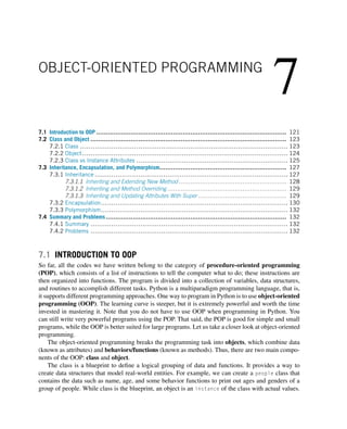
![122 CHAPTER 7 OBJECT-ORIENTED PROGRAMMING
For example, a person named “Iron man” with age 35. Put it another way, a class is like a template
to define the needed information, and an object is one specific copy that filled in the template. Also,
objects instantiated from the same class are independent from each other. For example, if we have
another person, say, “Batman” with age 33, it can be instantiated from the people class, but it remains
an independent instance.
To implement the above example in Python, see the code below. Do not worry if you do not under-
stand the syntax; the next section provides more helpful examples.
In [1]: class People():
def __init__(self, name, age):
self.name = name
self.age = age
def greet(self):
print(Greetings, + self.name)
In [2]: person1 = People(name = Iron Man, age = 35)
person1.greet()
print(person1.name)
print(person1.age)
Greetings, Iron Man
Iron Man
35
In [3]: person2 = People(name = Batman, age = 33)
person2.greet()
print(person2.name)
print(person2.age)
Greetings, Batman
Batman
33
In the above code example, we first defined a class, People, with name and age as the data, and a
method greet. We then instantiated an object, person1 with the specific name and age. We can clearly
see that the class defines the whole structure, while the object is just an instance of the class.
The many benefits of using OOP are as follows: It provides a clear modular structure for pro-
grams that enhances code reusability. It provides a simple way to solve complex problems. It helps
define more abstract data types to model real-world scenarios. It hides implementation details, leaving
a clearly defined interface. It combines data and operations.
There are also other advantages of using OOP in a large project. We encourage you to search online
to find out more. At this point, you may still not fully understand OOP’s advantages until you are
involved in complex large projects. We will continue to learn more about OOP during the course of
this book, and its usefulness will become apparent.](https://image.slidesharecdn.com/pythonprogrammingandnumericalmethodsaguideforengineersand-231017183839-0fbc5295/85/Python_Programming_and_Numerical_Methods_A_Guide_for_Engineers_and-pdf-135-320.jpg)
![7.2 CLASS AND OBJECT 123
7.2 CLASS AND OBJECT
The previous section introduced the two main components of OOP: class, which is a blueprint used to
define a logical grouping of data and functions, and object, which is an instance of the defined class
with actual values. In this section, we will get into greater detail of both of these components.
7.2.1 CLASS
A class is a definition of the structure that we want. Similar to a function, it is defined as a block of
code, starting with the class statement. The syntax of defining a class is:
class ClassName(superclass):
def __init__(self, arguments):
# define or assign object attributes
def other_methods(self, arguments):
# body of the method
Note that the definition of a class is very similar to a function. It needs to be instantiated first before
you can use it. For the class name, it is standard convention to use CapWords. The superclass is used
when you want create a new class to inherit the attributes and methods from another already defined
class. We will talk more about inheritance in the next section. The __init__ is one of the special
methods in Python classes that is run as soon as an object of a class is instantiated (created). It assigns
initial values to the object before it is ready to be used. Note the two underscores at the beginning and
end of the init, indicating this is a special method reserved for special use in the language. In this init
method, you can assign attributes directly when you create the object. The other_methods functions
are used to define the instance methods that will be applied on the attributes, just like functions we
discussed before. You may notice that there is an argument self for defining this method in the class.
Why? A class instance method must have this extra argument as the first argument when you define
it. This particular argument refers to the object itself; conventionally, we use self to name it. Instance
methods can freely access attributes and other methods in the same object by using this self parameter.
See the example below.
EXAMPLE: Define a class named Student, with the attributes sid (student id), name, gender,
type in the init method, and a method called say_name to print out the student’s name. All
attributes will be passed in except type, which will have a value as learning.
In [1]: class Student():
def __init__(self, sid, name, gender):
self.sid = sid
self.name = name
self.gender = gender](https://image.slidesharecdn.com/pythonprogrammingandnumericalmethodsaguideforengineersand-231017183839-0fbc5295/85/Python_Programming_and_Numerical_Methods_A_Guide_for_Engineers_and-pdf-136-320.jpg)
![124 CHAPTER 7 OBJECT-ORIENTED PROGRAMMING
self.type = learning
def say_name(self):
print(My name is + self.name)
From the above example, we can see this simple class contains all the necessary parts mentioned
previously. The __init__ method will initialize the attributes when we create an object. We need to
pass in the initial value for sid, name, and gender, while the attribute type is a fixed value as learning.
These attributes can be accessed by all the other methods defined in the class with self.attribute, for
example, in the say_name method, we can use the name attribute with self.name. The methods defined
in the class can be accessed and used in other different methods as well using self.method. Let us see
the following example.
TRY IT! Add a method report that prints not only the student name, but also the student id. The
method will have another parameter, score, that will pass in a number between 0 and 100 as part
of the report.
In [2]: class Student():
def __init__(self, sid, name, gender):
self.sid = sid
self.name = name
self.gender = gender
self.type = learning
def say_name(self):
print(My name is + self.name)
def report(self, score):
self.say_name()
print(My id is: + self.sid)
print(My score is: + str(score))
7.2.2 OBJECT
As mentioned before, an object is an instance of the defined class with actual values. Many instances of
different values associated with the class are possible, and each of these instances will be independent
with each other (as seen previously). Also, after we create an object and call this instance method from
the object, we do not need to give value to the self parameter because Python automatically provides
it; see the following example.](https://image.slidesharecdn.com/pythonprogrammingandnumericalmethodsaguideforengineersand-231017183839-0fbc5295/85/Python_Programming_and_Numerical_Methods_A_Guide_for_Engineers_and-pdf-137-320.jpg)
![7.2 CLASS AND OBJECT 125
EXAMPLE: Create two objects (001, Susan, F) and (002, Mike, M), and call
the method say_name.
In [3]: student1 = Student(001, Susan, F)
student2 = Student(002, Mike, M)
student1.say_name()
student2.say_name()
print(student1.type)
print(student1.gender)
My name is Susan
My name is Mike
learning
F
In the above code, we created two objects, student1 and student2, with two different sets of values.
Each object is an instance of the Student class and has a different set of attributes. Type student1.+TAB
to see the defined attributes and methods. To get access to one attribute, type object.attribute, e.g.,
student1.type. In contrast, to call a method, you need the parentheses because you are calling a
function, such as student1.say_name().
TRY IT! Call method report for student1 and student2 with scores of 95 and 90, respectively.
Note that we do not need the “self” as an argument here.
In [4]: student1.report(95)
student2.report(90)
My name is Susan
My id is: 001
My score is: 95
My name is Mike
My id is: 002
My score is: 90
We can see both methods calling to print out the data associated with the two objects. Note that the
score value we passed in is only available to the method report (within the scope of this method). We
can also see that the method say_name call in the report also works, as long as you call the method
with the self in it.
7.2.3 CLASS VS INSTANCE ATTRIBUTES
The attributes we presented above are actually called instance attributes, which means that they are
only belong to a specific instance; when you use them, you need to use the self.attribute within](https://image.slidesharecdn.com/pythonprogrammingandnumericalmethodsaguideforengineersand-231017183839-0fbc5295/85/Python_Programming_and_Numerical_Methods_A_Guide_for_Engineers_and-pdf-138-320.jpg)
![126 CHAPTER 7 OBJECT-ORIENTED PROGRAMMING
the class. There are other attributes called class attributes, which will be shared with all the instances
created from this class. Let us see an example how to define and use a class attribute.
EXAMPLE: Modify the Student class to add a class attribute n, which will record how many
object we are creating. Also, add a method num_instances to print out the number.
In [5]: class Student():
n = 0
def __init__(self, sid, name, gender):
self.sid = sid
self.name = name
self.gender = gender
self.type = learning
Student.n += 1
def say_name(self):
print(My name is + self.name)
def report(self, score):
self.say_name()
print(My id is: + self.sid)
print(My score is: + str(score))
def num_instances(self):
print(fWe have {Student.n}-instance in total)
In defining a class attribute, we must define it outside of all the other methods without using
self. To use the class attributes, we use ClassName.attribute, which in this case is Student.n. This
attribute will be shared with all the instances that are created from this class. Let us see the following
code to show the idea.
In [6]: student1 = Student(001, Susan, F)
student1.num_instances()
student2 = Student(002, Mike, M)
student1.num_instances()
student2.num_instances()
We have 1-instance in total
We have 2-instance in total
We have 2-instance in total
As before, we created two objects, the instance attribute sid, name, but gender only belongs to the
specific object. For example, student1.name is “Susan” and student2.name is “Mike”. But when we](https://image.slidesharecdn.com/pythonprogrammingandnumericalmethodsaguideforengineersand-231017183839-0fbc5295/85/Python_Programming_and_Numerical_Methods_A_Guide_for_Engineers_and-pdf-139-320.jpg)
![7.3 INHERITANCE, ENCAPSULATION, AND POLYMORPHISM 127
print the class attribute Student.n_instances out after we created object student2, the one in the
student1 changes as well. This is the expectation we have for the class attribute because it is shared
across all the created objects.
Now that we understand the difference between class and instance, we are in good shape to use basic
OOP in Python. Before we can take full advantage of OOP, we still need to understand the concept of
inheritance, encapsulation, and polymorphism. Let us start the next section!
7.3 INHERITANCE, ENCAPSULATION, AND POLYMORPHISM
We have already seen the modeling power of OOP using the class and object functions by combin-
ing data and methods. There are three more important concepts: (1) inheritance, which makes the
OOP code more modular, easier to reuse, and capable of building a relationship between classes;
(2) encapsulation, which can hide some of the private details of a class from other objects; and
(3) polymorphism, which allows us to use a common operation in different ways. A brief discussion
of how these concepts is discussed below.
7.3.1 INHERITANCE
Inheritance allows us to define a class that inherits all the methods and attributes from another class.
Convention denotes the new class as child class, and the one that it inherits from is called the parent
class or superclass. If we refer back to the definition of class structure, we can see the structure for
basic inheritance is class ClassName(superclass), which means the new class can access all the
attributes and methods from the superclass. Inheritance builds a relationship between the child and
parent classes. Usually, the parent class is a general type while the child class is a specific type. An
example is presented below.
TRY IT! Define a class named Sensor with attributes name, location, and record_date that pass
from the creation of an object and an attribute data as an empty dictionary to store data. Create
one method add_data with t and data as input parameters to take in timestamp and data arrays.
Within this method, assign t and data to the data attribute with “time” and “data” as the keys. In
addition, create one clear_data method to delete the data.
In [1]: class Sensor():
def __init__(self, name, location, record_date):
self.name = name
self.location = location
self.record_date = record_date
self.data = {}
def add_data(self, t, data):
self.data[time] = t](https://image.slidesharecdn.com/pythonprogrammingandnumericalmethodsaguideforengineersand-231017183839-0fbc5295/85/Python_Programming_and_Numerical_Methods_A_Guide_for_Engineers_and-pdf-140-320.jpg)
![128 CHAPTER 7 OBJECT-ORIENTED PROGRAMMING
self.data[data] = data
print(fWe have {len(data)} points saved)
def clear_data(self):
self.data = {}
print(Data cleared!)
Now we have a class to store general sensor information, we can create a sensor object to store data.
EXAMPLE: Create a sensor object.
In [2]: import numpy as np
sensor1 = Sensor(sensor1, Berkeley, 2019-01-01)
data = np.random.randint(-10, 10, 10)
sensor1.add_data(np.arange(10), data)
sensor1.data
We have 10 points saved
Out[2]: {time: array([0, 1, 2, 3, 4, 5, 6, 7, 8, 9]),
data: array([ 3, 2, 5, -1, 2, -2, 6, -1, 5, 4])}
7.3.1.1 Inheriting and Extending New Method
Suppose we have one different type of sensor, an accelerometer. It shares the same attributes and
methods as Sensor class, but it also has different attributes or methods that need to be appended or
modified from the original class. What should we do? Do we create a different class from scratch? This
is where inheritance can be used to make life easier. This new class will inherit from the Sensor class
with all the attributes and methods. We can think whether we want to extend the attributes or methods.
Let us first create this new class, Accelerometer, and add a new method, show_type, to report what
kind of sensor it is.
In [3]: class Accelerometer(Sensor):
def show_type(self):
print(I am an accelerometer!)
acc = Accelerometer(acc1, Oakland, 2019-02-01)
acc.show_type()
data = np.random.randint(-10, 10, 10)
acc.add_data(np.arange(10), data)
acc.data](https://image.slidesharecdn.com/pythonprogrammingandnumericalmethodsaguideforengineersand-231017183839-0fbc5295/85/Python_Programming_and_Numerical_Methods_A_Guide_for_Engineers_and-pdf-141-320.jpg)
![7.3 INHERITANCE, ENCAPSULATION, AND POLYMORPHISM 129
I am an accelerometer!
We have 10 points saved
Out[3]: {time: array([0, 1, 2, 3, 4, 5, 6, 7, 8, 9]),
data: array([ -1, 4, 7, -10, -2, -6, 2, -8, 9, 3])}
Creating this new Accelerometer class is very simple. It inherits from Sensor (denoted as a su-
perclass), and the new class actually contains all the attributes and methods from the superclass. We
then add a new method, show_type, which does not exist in the Sensor class, but we can successfully
extend the child class by adding the new method. This shows the power of inheritance: we have reused
most part of the Sensor class in a new class, and extended the functionality. Basically, the inheritance
sets up a logical relationship for the modeling of the real-world entities: the Sensor class as the parent
class is more general and passes all the characteristics to the child class Accelerometer.
7.3.1.2 Inheriting and Method Overriding
When we inherit from a parent class, we can change the implementation of a method provided by the
parent class; this is called method overriding and is shown in the example below.
EXAMPLE: Create a class UCBAcc (a specific type of accelerometer that was created at UC
Berkeley) that inherits from Accelerometer but replaces the show_type method that also prints
out the name of the sensor.
In [4]: class UCBAcc(Accelerometer):
def show_type(self):
print(fI am {self.name}, created at Berkeley!)
acc2 = UCBAcc(UCBAcc, Berkeley, 2019-03-01)
acc2.show_type()
I am UCBAcc, created at Berkeley!
We see that our new UCBAcc class actually overrides the method show_type with new features. In
this example, we are not only inheriting features from our parent class, but we are also modifying/im-
proving some methods.
7.3.1.3 Inheriting and Updating Attributes With Super
Let us create a class NewSensor that inherits from Sensor class, but is updated the attributes by adding
a new attribute brand. Of course, we can redefine the whole __init__ method as shown below that is
capable of overriding the parent function.](https://image.slidesharecdn.com/pythonprogrammingandnumericalmethodsaguideforengineersand-231017183839-0fbc5295/85/Python_Programming_and_Numerical_Methods_A_Guide_for_Engineers_and-pdf-142-320.jpg)
![130 CHAPTER 7 OBJECT-ORIENTED PROGRAMMING
In [5]: class NewSensor(Sensor):
def __init__(self,name,location,record_date,brand):
self.name = name
self.location = location
self.record_date = record_date
self.brand = brand
self.data = {}
new_sensor = NewSensor(OK, SF, 2019-03-01, XYZ)
new_sensor.brand
Out[5]: XYZ
There is a better way to achieve the same result. If we use the super method, we can avoid referring
to the parent class explicitly, as shown in the following example:
EXAMPLE: Redefine the attributes in inheritance.
In [6]: class NewSensor(Sensor):
def __init__(self,name,location,record_date,brand):
super().__init__(name, location, record_date)
self.brand = brand
new_sensor = NewSensor(OK, SF, 2019-03-01, XYZ)
new_sensor.brand
Out[6]: XYZ
Now we can see with the super method, we have avoided listing all of the definition of the attributes;
this helps keep your code maintainable for the foreseeable future. Because the child class does not
implicitly call the __init__ of the parent class, we must use super().__init__, as shown above.
7.3.2 ENCAPSULATION
Encapsulation is one of the fundamental concepts in OOP. It describes the idea of restricting access to
methods and attributes in a class. Encapsulation hides complex details from the users and prevents data
being modified by accident. In Python, this is achieved by using private methods or attributes using the
underscore as prefix, i.e., single “_” or double “__”, as shown the following example.
EXAMPLE:
In [7]: class Sensor():
def __init__(self, name, location):
self.name = name](https://image.slidesharecdn.com/pythonprogrammingandnumericalmethodsaguideforengineersand-231017183839-0fbc5295/85/Python_Programming_and_Numerical_Methods_A_Guide_for_Engineers_and-pdf-143-320.jpg)
![7.3 INHERITANCE, ENCAPSULATION, AND POLYMORPHISM 131
self._location = location
self.__version = 1.0
# a getter function
def get_version(self):
print(fThe sensor version is {self.__version})
# a setter function
def set_version(self, version):
self.__version = version
In [8]: sensor1 = Sensor(Acc, Berkeley)
print(sensor1.name)
print(sensor1._location)
print(sensor1.__version)
Acc
Berkeley
--------------------------------------------------------
AttributeError Traceback (most recent call last)
ipython-input-8-ca9b481690ba in module
2 print(sensor1.name)
3 print(sensor1._location)
---- 4 print(sensor1.__version)
AttributeError: 'Sensor' object has no attribute '__version'
The above example shows how the encapsulation works. With single underscore, we defined a
private variable that should not be accessed directly. Note that this is convention and nothing stops you
from actually accessing it. With double underscores, we can see that the attribute __version cannot be
accessed or modified directly. To get access to the double underscore attributes, we need to use “getter”
and “setter” functions to access it internally. A “getter” function is shown in the following example.
In [9]: sensor1.get_version()
The sensor version is 1.0](https://image.slidesharecdn.com/pythonprogrammingandnumericalmethodsaguideforengineersand-231017183839-0fbc5295/85/Python_Programming_and_Numerical_Methods_A_Guide_for_Engineers_and-pdf-144-320.jpg)
![132 CHAPTER 7 OBJECT-ORIENTED PROGRAMMING
In [10]: sensor1.set_version(2.0)
sensor1.get_version()
The sensor version is 2.0
The single and double underscore(s) apply to private methods as well, which are not discussed
because they are similar to the private attributes.
7.3.3 POLYMORPHISM
Polymorphism is another fundamental concept in OOP, which means multiple forms. Polymorphism
allows the use of a single interface with different underlying forms, such as data types or classes. For
example, we can have commonly named methods across classes or child classes. We have already seen
one example above when we overrode the method show_type in the UCBAcc. Both the parent class
Accelerometer and child class UCBAcc have a method named show_type, but they are implemented
differently. This ability of using a single name with many forms acting differently in different situations
greatly reduces our complexities. We will not expand this discussion on polymorphism, if you are
interested, check more online to get a deeper understanding.
7.4 SUMMARY AND PROBLEMS
7.4.1 SUMMARY
1. OOP and POP are different. OOP has many benefits and is often more appropriate for use in large-
scale projects.
2. Class is the blueprint of the structure that allows us to group data and methods, while object is an
instance from the class.
3. The concept of “inheritance” is key to OOP, which allows us to refer attributes or methods from the
superclass.
4. The concept of “encapsulation” allows us to hide some of the private details of a class from other
objects.
5. The concept of “polymorphism” allows us to use a common operation in different ways for different
data input.
7.4.2 PROBLEMS
1. Describe the differences between classes and objects.
2. Describe why we use “self” as the first argument in a method.
3. What is a constructor? And why do we use it?
4. Describe the differences between class and instance attributes.
5. The following is a definition of the class Point that takes in the coordinates x, y. Add a method
plot_point that plots the position of a point.](https://image.slidesharecdn.com/pythonprogrammingandnumericalmethodsaguideforengineersand-231017183839-0fbc5295/85/Python_Programming_and_Numerical_Methods_A_Guide_for_Engineers_and-pdf-145-320.jpg)
![7.4 SUMMARY AND PROBLEMS 133
import matplotlib.pyplot as plt
class Point():
def __init__(self, x, y):
self.x = x
self.y = y
6. Use the class from Problem 5 and add a method calculate_dist which takes in x and y from
another point, and returns the distance calculated between the two points.
7. What’s inheritance?
8. How do we inherit from a superclass and add new methods?
9. When we inherit from a superclass, we need to replace a method with a new one; how do we do
that?
10. What’s the super method? Why do we need it?
11. Create a class to model some real world objects and create a new class to inherit from it. See the
example below. You should use a different example and incorporate as many of the concepts we’ve
learned so far as possible.
In [1]: class Car():
def __init__(self, brand, color):
self.brand = brand
self.color = color
def start_my_car(self):
print(I am ready to drive!)
class Truck(Car):
def __init__(self, brand, color, size):
super().__init__(brand, color)
self.size = size
def start_my_car(self, key):
if key == truck_key:
print(I am ready to drive!)
else:
print(Key is not right)
def stop_my_car(self, brake):
if brake:
print(The engine is stopped!)
else:
print(I am still running!)](https://image.slidesharecdn.com/pythonprogrammingandnumericalmethodsaguideforengineersand-231017183839-0fbc5295/85/Python_Programming_and_Numerical_Methods_A_Guide_for_Engineers_and-pdf-146-320.jpg)

![8
COMPLEXITY
8.1 Complexity and Big-O Notation ..................................................................................... 135
8.2 Complexity Matters ................................................................................................... 137
8.3 The Profiler............................................................................................................. 139
8.3.1 Using the Magic Command .......................................................................... 139
8.3.2 Use Python Profiler ................................................................................... 140
8.3.3 Use Line Profiler....................................................................................... 141
8.4 Summary and Problems.............................................................................................. 142
8.4.1 Summary ............................................................................................... 142
8.4.2 Problems ............................................................................................... 142
8.1 COMPLEXITY AND BIG-O NOTATION
The complexity of a function is the relationship between the size of the input and the difficulty of
running the function to completion. The size of the input is usually denoted by n. However, n usually
describes something more tangible, such as the length of an array. The difficulty of a problem can
be measured in several ways. One suitable way to describe the difficulty of the problem is to use
basic operations: additions, subtractions, multiplications, divisions, assignments, and function calls.
Although each basic operation takes different amount of time, the number of basic operations needed
to complete a function is sufficiently related to the running time to be useful, and it is much easier to
count.
TRY IT! Count the number of basic operations, in terms of n, required for the following function
to terminate:
In [1]: def f(n):
out = 0
for i in range(n):
for j in range(n):
out += i*j
return out
Let us calculate the number of operations:
n2 additions; 0 subtractions; n2 multiplications; 0 divisions; 2n2 + 1 assignments; 0 function calls;
4n2 + 1 in total.](https://image.slidesharecdn.com/pythonprogrammingandnumericalmethodsaguideforengineersand-231017183839-0fbc5295/85/Python_Programming_and_Numerical_Methods_A_Guide_for_Engineers_and-pdf-148-320.jpg)
![136 CHAPTER 8 COMPLEXITY
The number of assignments is 2n2 + n + 1 because the line out += i*j is evaluated n2 times, j is
assigned n2 times, i is assigned n times, and the line out = 0 is assigned once. So, the complexity of
the function f can be described as 4n2 + n + 1.
A common notation for complexity is called Big-O notation. Big-O notation establishes the rela-
tionship in the growth of the number of basic operations with respect to the size of the input as the input
size becomes very large. Because hardware may be different on every machine, we cannot accurately
calculate how long it will take to complete without also evaluating the hardware, which is only valid
for that specific machine. How long it takes to calculate a specific set of input on a specific machine is
not germane. What is germane is the “time to completion.” Because this type of analysis is hardware
independent, the basic operations grow in direct response to the increase in the size of the input. As n
gets large, the highest power dominates; therefore, only the highest power term is included in Big-O
notation. Additionally, coefficients are not required to characterize growth, and so coefficients are also
dropped. In the previous example, we counted 4n2 + n + 1 basic operations to complete the function.
In Big-O notation we would say that the function is O(n2) (pronounced “O of n-squared”). We say
that any algorithm with complexity O(nc) where c is some constant with respect to n is polynomial
time.
TRY IT! Determine the complexity of the iterative Fibonacci function in Big-O notation.
In [2]: def my_fib_iter(n):
out = [1, 1]
for i in range(2, n):
out.append(out[i - 1] + out[i - 2])
return out
Since the only lines of code that take more time as n grows are those in the for-loop, we can restrict
our attention to the for-loop and the code block within it. The code within the for-loop does not grow
with respect to n (i.e., it is constant). Therefore, the number of basic operations is Cn, where C is some
constant representing the number of basic operations that occur in the for-loop, and these C operations
run n times. This gives a complexity of O(n) for my_fib_iter.
Assessing the exact complexity of a function can be difficult. In these cases, it might be sufficient
to give an upper bound or even an approximation of the complexity.
TRY IT! Give an upper bound on the complexity of the recursive implementation of Fibonacci.
Do you think it is a good approximation of the upper bound? Do you think that recursive Fibonacci
can possibly be polynomial time?
In [3]: def my_fib_rec(n):
if n 2:
out = 1](https://image.slidesharecdn.com/pythonprogrammingandnumericalmethodsaguideforengineersand-231017183839-0fbc5295/85/Python_Programming_and_Numerical_Methods_A_Guide_for_Engineers_and-pdf-149-320.jpg)
![8.2 COMPLEXITY MATTERS 137
else:
out = my_fib_rec(n-1) + my_fib_rec(n-2)
return out
As n gets large, we can say that the vast majority of function calls make two other function calls:
one addition and one assignment to the output. The addition and assignment do not grow with n per
function call, so we can ignore them in Big-O notation. However, the number of function calls grows
approximately by 2n , and so the complexity of my_fib_rec is upper bounded by O(2n).
There is an on-going debate whether or not O(2n) is a good approximation for the Fibonacci func-
tion.
Since the number of recursive calls grows exponentially with n, there is no way the recursive Fi-
bonacci function can be polynomial. That is, for any c, there is an n such that my_fib_rec takes more
than O(nc) basic operations to complete. Any function that is O(cn) for some constant c is said to be
exponential time.
TRY IT! What is the complexity of the following function in Big-O notation?
In [4]: def my_divide_by_two(n):
out = 0
while n 1:
n /= 2
out += 1
return out
Again, only the while-loop runs longer for larger n, so we can restrict our attention there. Within
the while-loop, there are two assignments: one division and one addition, both of which are constant
time with respect to n. So the complexity depends only on how many times the while-loop runs.
The while-loop cuts n in half in every iteration until n is less than 1. So the number of iterations,
I, is the solution to the equation n
2I = 1. With some manipulation, the solution is I = logn, so the
complexity of my_divide_by_two is O(logn). If we recall log rules, it does not matter what the base of
the log is because all logs are a scalar multiple of each other. Any function with complexity O(logn)
is said to be log-time.
8.2 COMPLEXITY MATTERS
So why does complexity matter? Because differing complexities require different amounts of time to
complete the task. Fig. 8.1 is a quick sketch showing you how the time changes with different input
size for complexity log(n), n, n2.
Let us look at another example. Assume you have an algorithm that runs in exponential time, say
O(2n), and let N be the largest problem you can solve with this algorithm using the computational](https://image.slidesharecdn.com/pythonprogrammingandnumericalmethodsaguideforengineersand-231017183839-0fbc5295/85/Python_Programming_and_Numerical_Methods_A_Guide_for_Engineers_and-pdf-150-320.jpg)
![8.3 THE PROFILER 139
algorithms exist for these problems. Examples of NP-complete problems include the Traveling Sales-
man, Set Cover, and Set Packing problems. Although theoretical in construction, solutions to these
problems have numerous applications in logistics and operations research. In fact, some encryption
algorithms that keep web and bank applications secure rely on the NP-completeness of breaking them.
A further discussion of NP-complete problems and the theory of complexity is beyond the scope of
this book, but these problems are very interesting and important to many engineering applications.
8.3 THE PROFILER
8.3.1 USING THE MAGIC COMMAND
Even if it does not change the Big-O complexity of a program, many programmers will spend long
hours to make their code run twice as fast or to gain even smaller improvements.
There are ways to check the run time of the code in the Jupyter notebook. Introduced below are the
magic commands to do that:
• %time: Get the run time of a single statement.
• %timeit: Get the repeated run time of a single statement.
• %%time: Get the run time of all the code in the cell.
• %%timeit: Get the repeated run time of a cell.
Note that the double percent magic command will measure the run time for all the code in a cell,
while the single percent command only works for a single statement.
In [1]: %time sum(range(200))
CPU times: user 6 µs, sys: 1 µs, total: 7 µs, wall time: 9.06 µs
Out[1]: 19900
In [2]: %timeit sum(range(200))
1.24 µs ± 70.6 ns per loop (mean ± std. dev. of 7 runs, 1000000 loops each)
In [3]: %%time
s = 0
for i in range(200):
s += i
CPU times: user 15 µs, sys: 0 ns, total: 15 µs, wall time: 17.9 µs
In [4]: %%timeit
s = 0](https://image.slidesharecdn.com/pythonprogrammingandnumericalmethodsaguideforengineersand-231017183839-0fbc5295/85/Python_Programming_and_Numerical_Methods_A_Guide_for_Engineers_and-pdf-152-320.jpg)
![140 CHAPTER 8 COMPLEXITY
for i in range(200):
s += i
7.06 µs ± 414 ns per loop (mean ± std. dev. of 7 runs, 100000 loops each)
WARNING! Sometimes it may not be proper to use the timeit, since it will run many loops for
the code, taking an inordinate amount of time to complete the task.
8.3.2 USE PYTHON PROFILER
You can also use the Python profiler (for additional discussion, read more in the Python documenta-
tion) to profile the code you write. In Jupyter notebook,
• %prun: Run a single statement through the Python code profiler.
• %%prun: Run a cell through the Python code profiler.
The following example sums random numbers over and over again:
In [6]: import numpy as np
In [7]: def slow_sum(n, m):
for i in range(n):
# we create a size m array of random numbers
a = np.random.rand(m)
s = 0
# in this loop we iterate through the array
# and add elements to the sum one by one
for j in range(m):
s += a[j]
In [8]: %prun slow_sum(1000, 10000)
The results are shown in Fig. 8.2.
The table shows the following columns (from Python profiler):
• ncalls is the number of calls;
• tottime is the total time spent in performing the given function (and excluding time made in calls
to subfunctions);
• percall is the quotient of dividing tottime by ncalls;
• cumtime is the total time spent in this and all subfunctions (from invocation till exit). This figure is
accurate even for recursive functions;
• percall is the quotient of dividing cumtime by primitive calls.](https://image.slidesharecdn.com/pythonprogrammingandnumericalmethodsaguideforengineersand-231017183839-0fbc5295/85/Python_Programming_and_Numerical_Methods_A_Guide_for_Engineers_and-pdf-153-320.jpg)
![8.3 THE PROFILER 141
FIGURE 8.2
The profiling result from prun.
8.3.3 USE LINE PROFILER
Many times we want to determine which line in a code script takes a long time so that we can rewrite
this line to make it more efficient. This can be done using the line_profiler, which will profile the
code line by line. This function is not shipped with Python; therefore, we need to install it, and then we
can use the magic command:
• %lprun: Run the line by line profile on a single statement.
In [9]: # Note, you only need run this once.
!conda install line_profiler
After you have installed this package, load the line_profiler extension:
In [10]: %load_ext line_profiler
The way we use the line_profiler to profile the code is shown as follows:
In [11]: %lprun -f slow_sum slow_sum(1000, 10000)
Running the above command will perform line by line profiling, as shown in Fig. 8.3.
The results include a summary for each line of the function. Note that lines 10 and 11 take the
majority of the total running time.
Usually when code takes longer to run than you would like, there is a bottleneck where a majority
of the time is being spent. That is, there is a line of code that is taking much longer to execute than
the other lines in the program. Addressing the bottleneck in a program will usually lead to the biggest
improvement in performance, even if there are other areas of your code that are more easily improved.
TIP! Start at the bottleneck when improving the performance of a code.](https://image.slidesharecdn.com/pythonprogrammingandnumericalmethodsaguideforengineersand-231017183839-0fbc5295/85/Python_Programming_and_Numerical_Methods_A_Guide_for_Engineers_and-pdf-154-320.jpg)
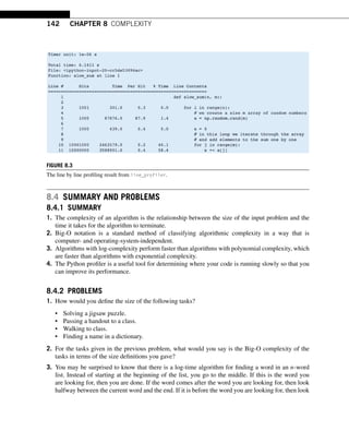
![8.4 SUMMARY AND PROBLEMS 143
halfway between the first word and the current word. Keep repeating this process until you find the
word. This algorithm is known as a binary search. It runs in log time because the search space is
cut in half at each iteration; therefore, it requires, at most, log2(n) iterations to find the word. Hence
the increase in run time is only a log in the length of the list.
There is a way to look up a word in O(1) or constant time. This means that no matter how long the
list is, it takes the same amount of time! Can you think of how this is done? Hint: Research hash
functions.
4. What is the complexity of the algorithms that compute the following recursive relationships? Clas-
sify the following algorithms as log time, polynomial time, or exponential time in terms of n given
that the implementation is (a) recursive and (b) iterative.
Tribonacci, T (n):
T (n) = T (n − 1) + T (n − 2) + T (n − 3)
T (1) = T (2) = T (3) = 1.
Timmynacci, t(n):
t(n) = t(n/2) + t(n/4)
t(n) = 1 if n 1.
5. What is the Big-O complexity of the Towers of Hanoi problem given in Chapter 6? Is the complexity
an upper bound or is it exact?
6. What is the Big-O complexity of the quicksort algorithm?
7. Run the following two iterative implementations of finding Fibonacci numbers in the line_pro-
filer as well as using the magic command to get the repeated run time. The first implementation
preallocates memory to an array that stores all the Fibonacci numbers. The second implementation
expands the list at each iteration of the for-loop.
In [ ]: import numpy as np
def my_fib_iter1(n):
out = np.zeros(n)
out[:2] = 1
for i in range(2, n):
out[i] = out[i-1] + out[i-2]
return out
def my_fib_iter2(n):
out = [1, 1]](https://image.slidesharecdn.com/pythonprogrammingandnumericalmethodsaguideforengineersand-231017183839-0fbc5295/85/Python_Programming_and_Numerical_Methods_A_Guide_for_Engineers_and-pdf-156-320.jpg)
![144 CHAPTER 8 COMPLEXITY
for i in range(2, n):
out.append(out[i-1]+out[i-2])
return np.array(out)](https://image.slidesharecdn.com/pythonprogrammingandnumericalmethodsaguideforengineersand-231017183839-0fbc5295/85/Python_Programming_and_Numerical_Methods_A_Guide_for_Engineers_and-pdf-157-320.jpg)
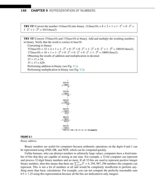
![9.2 FLOATING POINT NUMBERS 147
FIGURE 9.2
Binary multiplication.
9.2 FLOATING POINT NUMBERS
The number of bits is usually fixed for any given computer. Using binary representation gives us an
insufficient range and precision of numbers to do relevant engineering calculations. To achieve the
range of values needed with the same number of bits, we use floating point numbers, or floats for short.
Instead of utilizing each bit as the coefficient of a power of 2, floats allocate bits to three different parts:
the sign indicator, s, which says whether a number is positive or negative; characteristic or exponent,
e, which is the power of 2; and the fraction, f , which is the coefficient of the exponent. Almost all
platforms map Python floats to the IEEE754 double precision for a total of 64 bits. One bit is allocated
to the sign indicator, 11 bits are allocated to the exponent, and 52 bits are allocated to the fraction. With
11 bits allocated to the exponent; this makes 2048 values that this number can use. Since we want to
be able to make very precise numbers, we want some of these values to represent negative exponents
(i.e., to allow numbers that are between 0 and 1 (base10)). To accomplish this, 1023 is subtracted from
the exponent to normalize it. The value subtracted from the exponent is commonly referred to as the
bias. The fraction is a number between 1 and 2. In binary, this means that the leading term will always
be 1, and, therefore, it is a waste of bits to store it. To save space, the leading 1 is dropped. In Python,
we can obtain the float information using the sys package as shown below:
In [1]: import sys
sys.float_info
Out[1]: sys.float_info(max=1.7976931348623157e+308, max_exp=1024,
max_10_exp=308, min=2.2250738585072014e-308,
min_exp=-1021, min_10_exp=-307, dig=15,
mant_dig=53, epsilon=2.220446049250313e-16,
radix=2, rounds=1)
A float can then be represented as n = (−1)s2e−1023(1 + f ), for 64-bit.](https://image.slidesharecdn.com/pythonprogrammingandnumericalmethodsaguideforengineersand-231017183839-0fbc5295/85/Python_Programming_and_Numerical_Methods_A_Guide_for_Engineers_and-pdf-160-320.jpg)
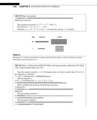
![9.2 FLOATING POINT NUMBERS 149
Therefore, the IEEE754 number
0 10000000010 1110000000000000000000000000000000000000000000000000
not only represents the number 15.0, but also all real numbers halfway between its immediate
neighbors. So any computation that has a result within this interval will be assigned as “15.0”.
We call the distance from one number to the next the gap. Because the fraction is multiplied by
2e−1023, the gap grows as the number represented grows. The gap at a given number can be computed
using the function spacing in NumPy.
TRY IT! Use the spacing function to determine the gap at 1e9. Verify that adding a number to
1e9 that is less than half the gap at 1e9 results in the same number.
In [2]: import numpy as np
In [3]: np.spacing(1e9)
Out[3]: 1.1920928955078125e-07
In [4]: 1e9 == (1e9 + np.spacing(1e9)/3)
Out[4]: True
There are special cases for the value of a floating point number when e = 0 (i.e., e =
00000000000(base2)) and when e = 2047, i.e., e = 11111111111(base2), which are reserved. When
the exponent is 0, the leading 1 in the fraction takes the value 0 instead. The result is a subnormal
number, which is computed by n = (−1)s2−1022(0 + f ) (note that it is −1022 instead of −1023).
When the exponent is 2047 and f is nonzero, then the result is “Not a Number,” which means that
the number is undefined. When the exponent is 2047, then f = 0 and s = 0, and the result is positive
infinity. When the exponent is 2047, then f = 0, and s = 1, and the result is minus infinity.
TRY IT! Compute the base10 value for
0 11111111110 1111111111111111111111111111111111111111111111111111
(IEEE754), the largest defined number for 64 bits, and for
0 00000000001 000000000000000000000000000000000000000000000000000
(IEEE754), the smallest. Note that to comply with the previously stated rules, the exponent
is e = 2046 and e = 1, respectively. Verify that Python agrees with these calculations using
sys.float_info.max and sys.float_info.min.
In [5]: l = (2**(2046-1023))*((1 + sum(0.5**np.arange(1, 53))))
l
Out[5]: 1.7976931348623157e+308](https://image.slidesharecdn.com/pythonprogrammingandnumericalmethodsaguideforengineersand-231017183839-0fbc5295/85/Python_Programming_and_Numerical_Methods_A_Guide_for_Engineers_and-pdf-162-320.jpg)
![150 CHAPTER 9 REPRESENTATION OF NUMBERS
In [6]: sys.float_info.max
Out[6]: 1.7976931348623157e+308
In [7]: s = (2**(1-1023))*(1+0)
s
Out[7]: 2.2250738585072014e-308
In [8]: sys.float_info.min
Out[8]: 2.2250738585072014e-308
Numbers that are larger than the largest floating point number capable of being represented result
in overflow; Python handles this case by assigning the result to inf. Numbers that are smaller than the
smallest subnormal number result in underflow; Python handles this case by assigning the result to
zero.
TRY IT! Show that adding the maximum 64-bit float number with 2 results in the same
number. Because the Python float does not have sufficient precision to store the + 2 for
sys.float_info.max, the operation is essentially equivalent to adding zero. Also show that
adding the maximum 64-bit float number with itself results in overflow, and that Python assigns
this overflow number to inf.
In [9]: sys.float_info.max + 2 == sys.float_info.max
Out[9]: True
In [10]: sys.float_info.max + sys.float_info.max
Out[10]: inf
TRY IT! The smallest subnormal number in a 64-bit number has
s = 0,e = 00000000000
and
f = 0000000000000000000000000000000000000000000000000001.
Using the special rules for subnormal numbers, this results in the subnormal number
(−1)021−10232−52 = 2−1074. Show that 2−1075 underflows to zero, and that the result cannot
be distinguished from zero. Show that 2−1074 does not.
In [11]: 2**(-1075)](https://image.slidesharecdn.com/pythonprogrammingandnumericalmethodsaguideforengineersand-231017183839-0fbc5295/85/Python_Programming_and_Numerical_Methods_A_Guide_for_Engineers_and-pdf-163-320.jpg)
![9.3 ROUND-OFF ERRORS 151
Out[11]: 0.0
In [12]: 2**(-1075) == 0
Out[12]: True
In [13]: 2**(-1074)
Out[13]: 5e-324
What have we gained by using IEEE754 versus binary? Using 64-bit binary gives us 264 numbers.
Since the number of bits does not change between binary and IEEE754, IEEE754 must also give us
264 numbers. In binary, numbers have a constant spacing between them. As a result, you cannot have
both range (i.e., large distance between minimum and maximum numbers capable of being represented)
and precision (i.e., small spacing between numbers). Controlling these parameters would depend on
where you put the decimal point in your number. IEEE754 overcomes this limitation by using very
high precision at small numbers and very low precision at large numbers. This limitation is usually
acceptable because the gap at large numbers is still small relative to the size of the number itself.
Therefore, even if the gap is millions large, it is irrelevant to normal calculations if the number under
consideration is in the trillions or higher.
This section introduced the representation of floating point numbers. This concept is described in
detail computer organization and design by David Patterson and John Hennessy.
9.3 ROUND-OFF ERRORS
In the previous section, we talked about how the floating-point numbers are represented in computers
as base2 fractions. This has a side effect that the floating-point numbers cannot be stored with perfect
precision; instead the numbers are approximated by a finite number of bytes. Therefore, the difference
between an approximation of a number used in computation and its correct (true) value is called a
round-off error. It is one of the common errors found usually in numerical calculations. The other
one is truncation error, which will be introduced in Chapter 18. The difference is that truncation
error is the error made by truncating an infinite sum and approximating it by a finite sum.
9.3.1 REPRESENTATION ERROR
The most common form of a round-off error is the representation error in the floating-point numbers.
A simple example will be how do we represent π? We know that π is an infinite number (i.e., has an
infinite number of digits); typically, we only use a finite number of digits. For example, if you only use
3.14159265, there will be an error between this approximation and the true infinite number. Another
example will be 1/3, the true value will be 0.333333333... No matter how many decimal digits we
choose, there is an round-off error as well.
When we round the numbers multiple times, the error will accumulate. For instance, if 4.845 is
rounded to two decimal places, it is 4.85. Then if we round it again to one decimal place, it is 4.9, the](https://image.slidesharecdn.com/pythonprogrammingandnumericalmethodsaguideforengineersand-231017183839-0fbc5295/85/Python_Programming_and_Numerical_Methods_A_Guide_for_Engineers_and-pdf-164-320.jpg)
![152 CHAPTER 9 REPRESENTATION OF NUMBERS
total error will be 0.55. But if we only round one time to one decimal place, it is 4.8, and the error is
0.045.
9.3.2 ROUND-OFF ERROR BY FLOATING-POINT ARITHMETIC
From the above example, the error between 4.845 and 4.8 should be 0.055. But if you calculate it in
Python, you will see the 4.9 − 4.845 is not equal to 0.055.
In [1]: 4.9 - 4.845 == 0.055
Out[1]: False
Why does this happen? If we take a second look at 4.9 − 4.845, we actually get
0.055000000000000604. This is because the floating point cannot be represented by the exact number
because it is an approximation; when it is used in arithmetic, it causes a small error.
In [2]: 4.9 - 4.845
Out[2]: 0.055000000000000604
In [3]: 4.8 - 4.845
Out[3]: -0.04499999999999993
Another example shows below that 0.1 + 0.2 + 0.3 is not equal to 0.6; the error is due to the same
cause.
In [4]: 0.1 + 0.2 + 0.3 == 0.6
Out[4]: False
Though the numbers cannot be made closer to their intended exact values, the round function can be
useful for post-rounding so that results with inexact values become comparable to one another:
In [5]: round(0.1 + 0.2 + 0.3, 5) == round(0.6, 5)
Out[5]: True
9.3.3 ACCUMULATION OF ROUND-OFF ERRORS
When we are doing a sequence of calculations on an initial input with round-off errors due to inexact
representation, the errors can be magnified or accumulated. As an example, if we have the number 1,
add and then subtract 1/3, it should give us 1. But if we add 1/3 and subtract the same number of times
1/3 over several iterations, do we still get the same number 1? No, we don’t. In the example below, the
more times you do this, the additional accumulates.](https://image.slidesharecdn.com/pythonprogrammingandnumericalmethodsaguideforengineersand-231017183839-0fbc5295/85/Python_Programming_and_Numerical_Methods_A_Guide_for_Engineers_and-pdf-165-320.jpg)
![9.4 SUMMARY AND PROBLEMS 153
In [6]: # If we only do once
1 + 1/3 - 1/3
Out[6]: 1.0
In [7]: def add_and_subtract(iterations):
result = 1
for i in range(iterations):
result += 1/3
for i in range(iterations):
result -= 1/3
return result
In [8]: # If we do this 100 times
add_and_subtract(100)
Out[8]: 1.0000000000000002
In [9]: # If we do this 1000 times
add_and_subtract(1000)
Out[9]: 1.0000000000000064
In [10]: # If we do this 10000 times
add_and_subtract(10000)
Out[10]: 1.0000000000001166
9.4 SUMMARY AND PROBLEMS
9.4.1 SUMMARY
1. Numbers may be represented in several different ways, each representation scheme having advan-
tages and disadvantages.
2. Computers must represent numbers using a finite number of digits (i.e., bits).
3. Binary and IEEE754 are finite representations of numbers used by computers.
4. The round-off error is an important error associated with numerical methods.
9.4.2 PROBLEMS
1. Write a function my_bin_2_dec(b) where b is a binary number represented by a list of ones and
zeros. The last element of b represents the coefficient of 20, the second-to-last element of b repre-](https://image.slidesharecdn.com/pythonprogrammingandnumericalmethodsaguideforengineersand-231017183839-0fbc5295/85/Python_Programming_and_Numerical_Methods_A_Guide_for_Engineers_and-pdf-166-320.jpg)
![154 CHAPTER 9 REPRESENTATION OF NUMBERS
sents the coefficient of 21, and so on. The output variable, d, should be the decimal representation
of b. Test cases are provided below.
In [ ]: def my_bin_2_dec(b):
# write your function code here
return d
In [ ]: # Output: 7
my_bin_2_dec([1, 1, 1])
In [ ]: # Output: 85
my_bin_2_dec([1, 0, 1, 0, 1, 0, 1])
In [ ]: # Output: 33554431
my_bin_2_dec([1]*25)
2. Write a function my_dec_2_bin(d) where d is a positive integer in decimal, and b is the binary
representation of d. The output b must be a list of ones and zeros, and the leading term must be a
1 unless the decimal input value is 0. Test cases are provided below.
In [ ]: def my_dec_2_bin(d):
# write your function code here
return b
In [ ]: # Output: [0]
my_dec_2_bin(0)
In [ ]: # Output: [1, 0, 1, 1, 1]
my_dec_2_bin(23)
In [ ]: # Output: [1, 0, 0, 0, 0, 0, 1, 1, 0, 0, 0, 1]
my_dec_2_bin(2097)
3. Use the two functions you wrote in Problems 1 and 2 to compute
d = my_bin_2_dec(my_dec_2_bin(12654)). Do you get the same number?
4. Write a function my_bin_adder(b1,b2) where b1, b2 and the output variable b are binary numbers
represented as in Problem 1. The output variable should be computed as b = b1 + b2. Do not
use your functions from Problems 1 and 2 to write this function (i.e., do not convert b1 and b2
to decimals; add them and then convert the result back to binary). This function should be able
to accept inputs b1 and b2 of any length (i.e., very long binary numbers), and b1 and b2 may not
necessarily be of the same length.
In [ ]: def my_bin_adder(b1, b2):
# write your function code here
return b
In [ ]: # Output: [1, 0, 0, 0, 0, 0]
my_bin_adder([1, 1, 1, 1, 1], [1])
In [ ]: # Output: [1, 1, 1, 0, 0, 1, 1]
my_bin_adder([1, 1, 1, 1, 1], [1, 0, 1, 0, 1, 0, 0])](https://image.slidesharecdn.com/pythonprogrammingandnumericalmethodsaguideforengineersand-231017183839-0fbc5295/85/Python_Programming_and_Numerical_Methods_A_Guide_for_Engineers_and-pdf-167-320.jpg)
![9.4 SUMMARY AND PROBLEMS 155
In [ ]: # Output: [1, 0, 1, 1]
my_bin_adder([1, 1, 0], [1, 0, 1])
5. What is the effect of allocating more bits to the fraction versus the characteristic, and vice versa?
What is the effect of allocating more bits to the sign?
6. Write a function my_ieee_2_dec(ieee) where ieee is a string that contains 64 characters of ones
and zeros, representing a 64-bit IEEE754 number. The output should be d, which is the equivalent
decimal representation of ieee. The input variable ieee will always be a 64-element string of ones
and zeros defining a 64-bit float.
In [ ]: def my_ieee_2_dec(ieee):
# Write your function here
return d
In [ ]: # Output: -48
ieee =1100000001001000000000000000000000000000000000000000000000000000
my_ieee_2_dec(ieee)
In [ ]: # Output: 3.39999999999999991118215802999
ieee =0100000000001011001100110011001100110011001100110011001100110011
my_ieee_2_dec(ieee)
7. Write a function my_dec_2_ieee(d) where d is a number in decimal, and the output variable ieee
is a string with 64 characters of ones and zeros, representing the 64-bit IEEE754 closest to d.
Assume that d will not cause an overflow for 64-bit ieee numbers.
In [ ]: def my_dec_2_ieee(d):
# write your function code here
return ieee
In [ ]: #Output:0100000000101110010111101010001110011100001100011010010001101000
d = 1.518484199625
my_dec_2_ieee(d)
In [ ]: #Output:1100000001110011010100100100010010010001001010011000100010010000
d = -309.141740
my_dec_2_ieee(d)
In [ ]: #Output:1100000011011000101010010000000000000000000000000000000000000000
d = -25252
my_dec_2_ieee(d)
8. Define ieee_baby to be a representation of numbers using 6 bits, where the first bit is the sign bit,
the second and third bits are allocated to the characteristic, and the fourth, fifth, and sixth bits are
allocated to the fraction. The normalization for the characteristic is 1.
Write all the decimal numbers that can be represented by ieee_baby. What is the largest/smallest
gap in ieee_baby?](https://image.slidesharecdn.com/pythonprogrammingandnumericalmethodsaguideforengineersand-231017183839-0fbc5295/85/Python_Programming_and_Numerical_Methods_A_Guide_for_Engineers_and-pdf-168-320.jpg)
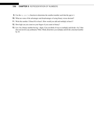
![10
ERRORS, GOOD
PROGRAMMING PRACTICES,
AND DEBUGGING
10.1 Error Types ........................................................................................................... 157
10.2 Avoiding Errors ...................................................................................................... 160
10.2.1 Plan Your Program ................................................................................. 160
10.2.2 Test Everything Often ............................................................................. 161
10.2.3 Keep Your Code Clean ............................................................................ 161
10.3 Try/Except............................................................................................................. 163
10.4 Type Checking ....................................................................................................... 166
10.5 Debugging ............................................................................................................ 168
10.5.1 Activating Debugger After Running Into an Exception ....................................... 168
10.5.2 Activating Debugger Before Running the Code................................................ 171
10.5.3 Add a Breakpoint .................................................................................. 172
10.6 Summary and Problems ............................................................................................ 173
10.6.1 Summary............................................................................................ 173
10.6.2 Problems ............................................................................................ 173
10.1 ERROR TYPES
We have noted errors before but have not yet talked about them in detail. There are three basic types
of errors that programmers need to be concerned about: syntax errors, runtime errors, and logical
errors. Syntax is the set of rules that govern a language. In written and spoken language, rules can
be bent or even broken to accommodate the speaker or writer. However, in a programming language
the rules are rigid. A syntax error occurs when the programmer writes an instruction using incorrect
syntax; Python cannot understand what you are saying. For example, 1 = x is not legal in the Python
programming language because numbers cannot be assigned as variables. If the programmer tries to
execute one of these instructions or any other syntactically incorrect statement, Python will return
an error message to the programmer and point out the location where the error occurred. Note that
although Python can identify the location where the syntax error is detected by the parser, it is possible
that the syntax error causing the error may be far away from the specific line identified.
EXAMPLE: Syntax error examples.
In [1]: 1 = x](https://image.slidesharecdn.com/pythonprogrammingandnumericalmethodsaguideforengineersand-231017183839-0fbc5295/85/Python_Programming_and_Numerical_Methods_A_Guide_for_Engineers_and-pdf-170-320.jpg)
![158 CHAPTER 10 ERRORS, GOOD PROGRAMMING PRACTICES, AND DEBUGGING
File ipython-input-1-7a7b257d8e3d, line 1
1 = x
ˆ
SyntaxError: can’t assign to literal
In [2]: (1]
File ipython-input-2-800df0a5e99c, line 1
(1]
ˆ
SyntaxError: invalid syntax
In [3]: if True
print(Here)
File ipython-input-3-025e9fce1ee3, line 1
if True
ˆ
SyntaxError: invalid syntax
The last line of the error message shows what happened – SyntaxError, and the lines before in-
dicate where the error happens in the context of the code. Overall, syntax errors are usually easily
detectable, found, and fixed.
Even if all the syntax is correct in your code, it may still cause an error during execution of the
code. Errors that occur during execution are called exceptions or runtime errors. Exceptions are
more difficult to find and are only detectable when a program is run. Note that exceptions are not fatal.
We will learn later how to handle them in Python. If we do not handle them, Python will terminate the
program. Let us see some examples below.
In [4]: 1/0
------------------------------------------------------
ZeroDivisionError Traceback (most recent call last)
ipython-input-4-9e1622b385b6 in module
---- 1 1/0](https://image.slidesharecdn.com/pythonprogrammingandnumericalmethodsaguideforengineersand-231017183839-0fbc5295/85/Python_Programming_and_Numerical_Methods_A_Guide_for_Engineers_and-pdf-171-320.jpg)
![10.1 ERROR TYPES 159
ZeroDivisionError: division by zero
In [5]: x = [2]
x + 2
-----------------------------------------------------
TypeError Traceback (most recent call last)
ipython-input-5-29a14b9fefb9 in module
1 x = [2]
---- 2 x + 2
TypeError: can only concatenate list (not int) to list
In [6]: print(a)
------------------------------------------------------
NameError Traceback (most recent call last)
ipython-input-6-bca0e2660b9f in module
---- 1 print(a)
NameError: name a is not defined
As shown in the examples above, there are different built-in exceptions: ZeroDivisionError,
TypeError, and NameError. You can find a complete list of built-in exceptions in the Python docu-
mentation.1 In addition, you can define your own exception types, but we will not deal with this herein;
if you are interested in how to define customized exceptions, check out the documentation.2
Most of the exceptions are easy to locate because Python will stop running and tell you where the
problem is. After programming a function, seasoned programmers will usually run the function several
times, allowing the function to “throw” any errors so that they can fix them. Note that no exception
does not mean the function works correctly.
1 https://docs.python.org/3/library/exceptions.html#bltin-exceptions.
2 https://docs.python.org/3/tutorial/errors.html#user-defined-exceptions.](https://image.slidesharecdn.com/pythonprogrammingandnumericalmethodsaguideforengineersand-231017183839-0fbc5295/85/Python_Programming_and_Numerical_Methods_A_Guide_for_Engineers_and-pdf-172-320.jpg)
![160 CHAPTER 10 ERRORS, GOOD PROGRAMMING PRACTICES, AND DEBUGGING
One of the most difficult errors to find are called logic errors. A logic error does not throw an error.
Although the program will run smoothly, it is an error because the output obtained is not the solution
you expect. For example, consider the following incorrect implementation of the factorial function.
In [7]: def my_bad_factorial(n):
out = 0
for i in range(1, n+1):
out = out*i
return out
In [8]: my_bad_factorial(4)
Out[8]: 0
This function will not produce a runtime error for any input that is valid for a correctly implemented
factorial function; however, if you try using my_bad_factorial, you will find that the answer is always
0 because out is initialized to 0 instead of 1. Therefore, the line out = 0 is a logic error. It does not
produce a runtime error by Python, but it leads to an incorrect computation.
Although the logic errors seem unlikely to occur—or at least as easy to find as other kinds of
errors—when programs become longer and more complicated, such errors are very easy to generate
and notoriously difficult to find. When logic errors occur, you have no choice but to meticulously comb
through each line of your code until you find the problem. For these cases, it is important to know
exactly how Python will respond to every command you give and not make any assumptions. You can
also use Python’s debugger, which will be described in the last section of this chapter.
10.2 AVOIDING ERRORS
There are many techniques that can help prevent errors and make it easier for you to find them when
they occur. Because becoming familiar with the types of mistakes common in programming is a “learn-
ing as you go” process; we cannot possibly list them all here. That said, we present a few of them in
the following section to help you build good habits.
10.2.1 PLAN YOUR PROGRAM
When writing an essay, it is important to have a structure and a direction that you intend to follow. To
help make your structure more tangible, writing an essay usually starts with an outline containing the
main points you wish to address in your paper. This is even more important to do when programming
because computers do not interpret what you write. When coding complicated programs, you should
start with an outline of your program that addresses all the tasks you want your program to perform
and in the order in which it should perform them.
Many novice programmers, eager to finish their assignments, will rush to the programming part
without properly planning out the tasks needed to accomplish the given task. Haphazard planning](https://image.slidesharecdn.com/pythonprogrammingandnumericalmethodsaguideforengineersand-231017183839-0fbc5295/85/Python_Programming_and_Numerical_Methods_A_Guide_for_Engineers_and-pdf-173-320.jpg)
![162 CHAPTER 10 ERRORS, GOOD PROGRAMMING PRACTICES, AND DEBUGGING
y=x**2
y=y+2*x
y=y+1
Even if the outcome is the same, every character you type is a chance that you will make a mistake;
therefore, reducing how much code you write will reduce your risk of introducing errors. Additionally,
writing a complete expression will help you and other people understand what you are doing. In the
previous example, in the first case it is clear that you are computing the value of a quadratic at x, while
in the second case it is not clear. You can also keep your code “clean” by using variables rather than
values.
EXAMPLE: Poor implementation of adding 10 random numbers.
In [1]: import numpy as np
s = 0
a = np.random.rand(10)
for i in range(10):
s = s + a[i]
EXAMPLE: Good implementation of adding 10 random numbers.
In [2]: n = 10
s = 0
a = np.random.rand(n)
for i in range(n):
s = s + a[i]
The second implementation is better for two reasons: first, it is easier for anyone reading your code
that n represents the number of random numbers you want to add up, and it appears rationally where
it is supposed to in the code (i.e., when creating the array of random numbers and when indexing
the array in the for-loop); and second, if you ever wanted to change the number of random numbers
you wish to add up, you would only have to change it in one place at the beginning. This reduces the
chances of making mistakes while writing the code and when changing the value of n.
Again, this is not critical for such a small piece of code, but it will become very important when
your code becomes more complicated and values must be reused many times.
EXAMPLE: An even better implementation of adding 10 random numbers.
In [3]: s = sum(np.random.rand(10))
When you become more familiar with Python, you will want to use as few lines as possible to do
the same job; therefore, familiarity of the common functions and how to use them will make your code
more concise and efficient.](https://image.slidesharecdn.com/pythonprogrammingandnumericalmethodsaguideforengineersand-231017183839-0fbc5295/85/Python_Programming_and_Numerical_Methods_A_Guide_for_Engineers_and-pdf-175-320.jpg)
![10.3 TRY/EXCEPT 163
You can also keep your code clean by assigning your variables short, descriptive names. For exam-
ple, as noted earlier, n is a sufficient variable for such a simple task. The variable name x is probably a
good name since x usually holds value of position rather than a number; but theNumberOfRandomNum-
bersToBeAdded is a poor variable name even though it is descriptive.
Finally, you can keep your code clean by commenting frequently. Although no commenting is
certainly bad practice, over-commenting can be equally bad practice. Different programmers will dis-
agree on exactly how much commenting is appropriate. It will be up to you to decide what level of
commenting is appropriate.
10.3 TRY/EXCEPT
Often it is important to write programs that can handle certain types of errors or exceptions gracefully.
More specifically, the error or exception must not cause a critical error that makes your program shut
down. A Try-Except statement is a code block that allows your program to take alternative actions in
case an error occurs.
CONSTRUCTION: Try-Exception Statement
try:
code block 1
except ExceptionName:
code block 2
Python will first attempt to execute the code in the try statement (code block 1). If no exception
occurs, the except statement is skipped and the execution of the try statement is finished. If any
exception occurs, the rest of the clause is skipped. Then if the exception type matches the exception
named after the except keyword (ExceptionName), the code in the except statement will be executed
(code block 2). If nothing in this block stops the program, it will continue to execute the rest of the
code outside of the try-except code blocks. If the exception does not match the ExceptionName, it is
passed on to outer try statements. If no other handler is found, then the execution stops with an error
message.
EXAMPLE: Capture the exception.
In [1]: x = 6
try:
if x 3:
print(X is larger than 3)
except TypeError:
print(Oops! x is not a valid number. Try again...)](https://image.slidesharecdn.com/pythonprogrammingandnumericalmethodsaguideforengineersand-231017183839-0fbc5295/85/Python_Programming_and_Numerical_Methods_A_Guide_for_Engineers_and-pdf-176-320.jpg)
![164 CHAPTER 10 ERRORS, GOOD PROGRAMMING PRACTICES, AND DEBUGGING
Oops! x is not a valid number. Try again...
EXAMPLE: If your handler is trying to capture another exception type that the except does not
capture, then an error occurs and the execution stops.
In [2]: x = 6
try:
if x 3:
print(X is larger than 3)
except ValueError:
print(Oops! x is not a valid number. Try again...)
------------------------------------------------------
TypeError Traceback (most recent call last)
ipython-input-2-899d928e7a1f in module
1 x = 6
2 try:
---- 3 if x 3:
4 print(X is larger than 3)
5 except ValueError:
TypeError: not supported between instances of str
and int
Of course, a try statement may have more than one except statement to handle different exceptions
or you cannot specify the exception type so that the except will catch any exception.
In [3]: x = s
try:
if x 3:
print(x)
except:
print(fSomething is wrong with x = {x})
Something is wrong with x = s](https://image.slidesharecdn.com/pythonprogrammingandnumericalmethodsaguideforengineersand-231017183839-0fbc5295/85/Python_Programming_and_Numerical_Methods_A_Guide_for_Engineers_and-pdf-177-320.jpg)
![10.3 TRY/EXCEPT 165
EXAMPLE: Handling multiple exceptions.
In [4]: def test_exceptions(x):
try:
x = int(x)
if x 3:
print(x)
except TypeError:
print(x was not a valid number. Try again...)
except ValueError:
print(Cannot convert x to int. Try again...)
except:
print(Unexpected error)
In [5]: x = [1, 2]
test_exceptions(x)
x was not a valid number. Try again...
In [6]: x = s
test_exceptions(x)
Cannot convert x to int. Try again...
Another useful thing in Python is that we can raise some exceptions in certain cases using raise.
For example, if we need x to be less than or equal to 5, we can use the following code to raise an
exception if x is larger than 5. The program will display our exception and stop the execution.
In [7]: x = 10
if x 5:
raise(Exception(x should be = 5))
--------------------------------------------------------
Exception Traceback (most recent call last)
ipython-input-7-99b32b52c4f8 in module
2
3 if x 5:
---- 4 raise(Exception(x should be = 5))](https://image.slidesharecdn.com/pythonprogrammingandnumericalmethodsaguideforengineersand-231017183839-0fbc5295/85/Python_Programming_and_Numerical_Methods_A_Guide_for_Engineers_and-pdf-178-320.jpg)
![166 CHAPTER 10 ERRORS, GOOD PROGRAMMING PRACTICES, AND DEBUGGING
Exception: x should be = 5
WARNING! Try-except statements should never be used in place of good programming prac-
tice. For example, you should not code sloppily and then encase your program in a try-except
statement until you have taken every measure you can think of to ensure that your function is
working properly.
10.4 TYPE CHECKING
Python is both a strongly and dynamically typed programming language. This means that any variable
can take on any data type at any time (this is dynamically typed part); however, once a variable is
assigned a type, it cannot change. For example, you can write x = 1 immediately followed by x = s
because Python is a dynamically typed language. You cannot run 3 + 5, because it is a strongly typed
language, i.e., the string 3 cannot convert in runtime to an integer. In statically typed programming
languages, you must declare what kind of data type your variable is to execute before you use it, and
the data type usage of your variable cannot change within the scope of a function.
In the case of Python, there is no way to ensure that the user of your function is inputting variables
of the data type you expect. For example, the function my_adder in Chapter 3 is designed to add three
numbers together. However, the user can input strings, lists, dictionaries, or functions, each of which
will cause different levels of problems. You can have your function type check the input variables
before continuing and force an error using the error function.
TRY IT! Modify my_adder to type check that the input variables are floats. If any of the input
variables are not floats, the function should return an appropriate error to the user using the raise
function. Try your function for erroneous input arguments to verify that they are checked.
In [1]: def my_adder(a, b, c):
# type check
if isinstance(a, float) and isinstance(b, float) and
isinstance(c, float):
pass
else:
raise(TypeError(Inputs must be floats))
out = a + b + c
return out
In [2]: my_adder(1.0, 2.0, 3.0)](https://image.slidesharecdn.com/pythonprogrammingandnumericalmethodsaguideforengineersand-231017183839-0fbc5295/85/Python_Programming_and_Numerical_Methods_A_Guide_for_Engineers_and-pdf-179-320.jpg)
![10.4 TYPE CHECKING 167
Out[2]: 6.0
In [3]: my_adder(1.0, 2.0, 3.0)
---------------------------------------------------
TypeError Traceback (most recent call last)
ipython-input-3-14e4b71b8c1d in module
---- 1 my_adder(1.0, 2.0, 3.0)
ipython-input-1-c2a54d39e3d9 in my_adder(a, b, c)
---- 6 raise(TypeError(Inputs must be floats))
7
8 out = a + b + c
9 return out
TypeError: Input arguments must be floats
In [4]: my_adder(1, 2, 3)
-----------------------------------------------------
Exception Traceback (most recent call last)
ipython-input-4-fc54adcab3d7 in module
---- 1 my_adder(1, 2, 3)
ipython-input-1-c2a54d39e3d9 in my_adder(a, b, c)
4 pass
5 else:
---- 6 raise(TypeError(Inputs must be floats))
7
8 out = a + b + c
TypeError: Inputs must be floats
Note that 1, 2, 3 are integers instead of floats, therefore, it raised an error message, and we need to
change the function to make sure that any numbers will be added.](https://image.slidesharecdn.com/pythonprogrammingandnumericalmethodsaguideforengineersand-231017183839-0fbc5295/85/Python_Programming_and_Numerical_Methods_A_Guide_for_Engineers_and-pdf-180-320.jpg)
![168 CHAPTER 10 ERRORS, GOOD PROGRAMMING PRACTICES, AND DEBUGGING
In [5]: def my_adder(a, b, c):
# type check
if isinstance(a, (float, int, complex)) and
isinstance(b, (float, int, complex)) and
isinstance(c, (float, int, complex)):
pass
else:
raise(TypeError(Inputs must be numbers))
out = a + b + c
return out
In [6]: my_adder(1, 2, 3)
Out[6]: 6
In [7]: my_adder(1.0, 2, 3)
Out[7]: 6.0
In [8]: my_adder(1j, 2+2j, 3+2j)
Out[8]: (5+5j)
10.5 DEBUGGING
Debugging is the process of systematically removing errors, or bugs, from your code. Python has
functionalities that can assist you when debugging. The standard debugging tool in Python is pdb
(Python DeBugger) for interactive debugging. It lets you step through the code line by line to find out
what might be causing a difficult error. The IPython version of this is ipdb (IPython DeBugger). We
will not cover too much about it herein; check out the documentation3 for details. In this section, basic
debug steps in Jupyter notebook will be introduced. We will show you how to use two really useful
magic commands %debug and %pdb to find the code causing trouble.
There are two ways you can debug your code: (1) activate the debugger when you run into an
exception; and (2) activate debugger before running the code.
10.5.1 ACTIVATING DEBUGGER AFTER RUNNING INTO AN EXCEPTION
If we run the code which stops at an exception, we can call %debug. For example, we have a function
that squares the input number and then adds to itself, as shown below:
3 https://docs.python.org/3/library/pdb.html.](https://image.slidesharecdn.com/pythonprogrammingandnumericalmethodsaguideforengineersand-231017183839-0fbc5295/85/Python_Programming_and_Numerical_Methods_A_Guide_for_Engineers_and-pdf-181-320.jpg)
![10.5 DEBUGGING 169
In [1]: def square_number(x):
sq = x**2
sq += x
return sq
In [2]: square_number(10)
-----------------------------------------------------
TypeError Traceback (most recent call last)
ipython-input-2-e0b77a2957d5 in module
---- 1 square_number(10)
ipython-input-1-3fc6a3900214 in square_number(x)
1 def square_number(x):
2
---- 3 sq = x**2
4 sq += x
5
TypeError: unsupported operand type(s) for ** or pow():
str and int
After we locate this exception, we can activate the debugger by using the magic command %debug,
which opens an interactive debugger, at which point you can type in commands in the debugger to get
useful information.
In [3]: %debug
ipython-input-1-3fc6a3900214(3)square_number()
1 def square_number(x):
2
---- 3 sq = x**2
4 sq += x
5](https://image.slidesharecdn.com/pythonprogrammingandnumericalmethodsaguideforengineersand-231017183839-0fbc5295/85/Python_Programming_and_Numerical_Methods_A_Guide_for_Engineers_and-pdf-182-320.jpg)
![10.5 DEBUGGING 171
10.5.2 ACTIVATING DEBUGGER BEFORE RUNNING THE CODE
We can also turn on the debugger before we run the code and then turn it off once we are finished
running the code.
In [4]: %pdb on
Automatic pdb calling has been turned ON
In [5]: square_number(10)
--------------------------------------------------------
TypeError Traceback (most recent call last)
ipython-input-5-e0b77a2957d5 in module
---- 1 square_number(10)
ipython-input-1-3fc6a3900214 in square_number(x)
1 def square_number(x):
2
---- 3 sq = x**2
4 sq += x
5
TypeError: unsupported operand type(s) for ** or pow():
str and int
ipython-input-1-3fc6a3900214(3)square_number()
1 def square_number(x):
2
---- 3 sq = x**2
4 sq += x
5
ipdb p x
10
ipdb c](https://image.slidesharecdn.com/pythonprogrammingandnumericalmethodsaguideforengineersand-231017183839-0fbc5295/85/Python_Programming_and_Numerical_Methods_A_Guide_for_Engineers_and-pdf-184-320.jpg)
![172 CHAPTER 10 ERRORS, GOOD PROGRAMMING PRACTICES, AND DEBUGGING
In [6]: # let’s turn off the debugger
%pdb off
Automatic pdb calling has been turned OFF
10.5.3 ADD A BREAKPOINT
It is often very useful to insert a breakpoint into your code. A breakpoint is a line in your code at which
Python will stop when the function is run.
In [7]: import pdb
In [8]: def square_number(x):
sq = x**2
# we add a breakpoint here
pdb.set_trace()
sq += x
return sq
In [9]: square_number(3)
ipython-input-8-e48ec2675aea(8)square_number()
- sq += x
(Pdb) l
3 sq = x**2
4
5 # we add a breakpoint here
6 pdb.set_trace()
7
8 - sq += x
9
10 return sq
[EOF]
(Pdb) p x
3
(Pdb) p sq
9](https://image.slidesharecdn.com/pythonprogrammingandnumericalmethodsaguideforengineersand-231017183839-0fbc5295/85/Python_Programming_and_Numerical_Methods_A_Guide_for_Engineers_and-pdf-185-320.jpg)
![10.6 SUMMARY AND PROBLEMS 173
(Pdb) c
Out[9]: 12
After we added pdb.set_trace(), the program stopped at this line and activated the pdb debugger.
We can now check all the variable values that were assigned before this line and use the command c to
continue the execution.
Using the Python’s debugger can be extremely helpful in finding and fixing errors in your code. We
encourage you to use the debugger for large programs.
10.6 SUMMARY AND PROBLEMS
10.6.1 SUMMARY
1. Errors are inevitable when coding. Errors are important because they tell you that something is not
working the way you intended.
2. There are three types of errors: syntax errors, exceptions, and logical errors.
3. You can reduce the numbers of errors in your coding with good coding practice.
4. Try-except statements can be used to handle exceptions without stopping your code.
5. The Debugger is a Python tool for helping you find errors.
10.6.2 PROBLEMS
None, have fun with what we learned in this chapter.](https://image.slidesharecdn.com/pythonprogrammingandnumericalmethodsaguideforengineersand-231017183839-0fbc5295/85/Python_Programming_and_Numerical_Methods_A_Guide_for_Engineers_and-pdf-186-320.jpg)
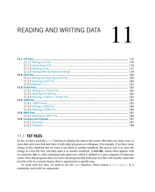
![176 CHAPTER 11 READING AND WRITING DATA
f = open(filename, mode)
The f above is the returned file object. The filename takes a string that tells the computer the
location of the file you want to open, and mode is another string containing a few characters, which
describes the way in which the file will be used. The common modes are:
• r, this is the default mode, which opens a file for reading.
• w, this mode opens a file for writing. If the file does not exist, it creates a new file.
• a, opens a file in append mode, so that you can append data to end of file. If the file does not exist,
it creates a new file.
• b, opens a file in binary mode.
• r+, opens a file (does not create) for reading and writing.
• w+, opens or creates a file for writing and reading, discards existing contents.
• a+, opens or creates a file for reading and writing, and appends data to the end of file.
11.1.1 WRITING TO A FILE
TRY IT! Create a text file called test.txt and write a couple lines in it.
In [1]: f = open(test.txt, w)
for i in range(5):
f.write(fThis is line {i}n)
f.close()
In the above code, we first opened a file object f with the file name test.txt. We used w for
the mode, which indicates we want to write code. We wrote five lines (note the newline n at the end
of the string), and then we closed the file object. The content of the file is shown in Fig. 11.1.
NOTE! It is good practice to close the file using f.close() at the end of the file. If you do not
close them yourself, Python will eventually close them for you. Note that sometimes when writing
to a file, the data may not write to disk until you close the file. The longer you keep the file open,
the greater the chance you will lose your data.
11.1.2 APPENDING A FILE
Next, we will append a string to the test.txt file. It is very similar to how we write the file, with only
one difference: we change the mode to a instead. See the results in Fig. 11.2.](https://image.slidesharecdn.com/pythonprogrammingandnumericalmethodsaguideforengineersand-231017183839-0fbc5295/85/Python_Programming_and_Numerical_Methods_A_Guide_for_Engineers_and-pdf-188-320.jpg)
![11.1 TXT FILES 177
FIGURE 11.1
The content in the text file we write.
FIGURE 11.2
Append a line to the end of an existing file.
In [2]: f = open(test.txt, a)
f.write(fThis is another linen)
f.close()
11.1.3 READING A FILE
We can read a file from disk and store all the contents to a variable. Let us read in the test.txt file we
created above and store all the contents in the file to a variable content.
In [3]: f = open(./test.txt, r)
content = f.read()](https://image.slidesharecdn.com/pythonprogrammingandnumericalmethodsaguideforengineersand-231017183839-0fbc5295/85/Python_Programming_and_Numerical_Methods_A_Guide_for_Engineers_and-pdf-189-320.jpg)
![178 CHAPTER 11 READING AND WRITING DATA
f.close()
print(content)
This is line 0
This is line 1
This is line 2
This is line 3
This is line 4
This is another line
In this way, we can store all the lines in the file into a one-string variable. To prove that this is a string,
we can verify that variable content.
In [4]: type(content)
Out[4]: str
Sometimes we want to read in the contents in the files line by line and store it in a list: using
f.readlines() will achieve this.
In [5]: f = open(./test.txt, r)
contents = f.readlines()
f.close()
print(contents)
[This is line 0n,This is line 1n,This is line 2n,
This is line 3n,This is line 4n,This is another linen]
In [6]: type(contents)
Out[6]: list
11.1.4 DEALING WITH NUMBERS AND ARRAYS
Since we will be working with numerical methods later and will often work with numbers or arrays,
we can use the above methods to save the numbers or arrays to a file and read it back to the memory.
Although viable, it is a bit clumsy. Instead, programmers commonly use the NumPy package to directly
save/read an array. An example is presented below.
TRY IT! Store an array [[1.20, 2.20, 3.00], [4.14, 5.65, 6.42]] to a file named my_ar-
ray.txt and read it back to a variable called my_arr.
In [7]: import numpy as np](https://image.slidesharecdn.com/pythonprogrammingandnumericalmethodsaguideforengineersand-231017183839-0fbc5295/85/Python_Programming_and_Numerical_Methods_A_Guide_for_Engineers_and-pdf-190-320.jpg)
![11.1 TXT FILES 179
In [8]: arr = np.array([[1.20, 2.20, 3.00], [4.14, 5.65, 6.42]])
arr
Out[8]: array([[1.2 , 2.2 , 3. ],
[4.14, 5.65, 6.42]])
In [9]: np.savetxt(my_arr.txt, arr, fmt=%.2f,
header = Col1 Col2 Col3)
The above example demonstrates how to save a 2D array into a text file using np.savetxt. The first
argument is the file name, the second argument is the object we wish to save, and the third argument
is to define the format for the output (we use %.2f to indicate we want the output numbers with two
decimals). The fourth argument is the header we wish to write into the file. See the results in Fig. 11.3.
FIGURE 11.3
The NumPy array we saved in the file.
In [10]: my_arr = np.loadtxt(my_arr.txt)
my_arr
Out[10]: array([[1.2 , 2.2 , 3. ],
[4.14, 5.65, 6.42]])
Reading the file directly into an array is very simple by using the np.loadtxt function, which skips
the first header. There are many different arguments that can control how a file is read. Additional
discussion on this topic will be explored in the next section; however, we are not going into much
detail herein beyond what is presented above. Check the documentation or use the question mark if
you need help.](https://image.slidesharecdn.com/pythonprogrammingandnumericalmethodsaguideforengineersand-231017183839-0fbc5295/85/Python_Programming_and_Numerical_Methods_A_Guide_for_Engineers_and-pdf-191-320.jpg)
![180 CHAPTER 11 READING AND WRITING DATA
11.2 CSV FILES
Often, scientific data are stored in the comma-separated values (CSV) file format, which is a delimited
text file that uses a comma to separate values. It is a very useful format that can store large tables of
data (numbers and text) in plain text. Each line (row) in the data is one data record, and each record
consists of one or more fields separated by commas. It also can be opened using Microsoft Excel to
visualize the rows and columns.
Python has its own CSV module to read and write a CSV file; we are not going to discuss this
further. Details on this module is available in the documentation.1 Instead, we will use the NumPy
package to deal with CSV files, because it is preferred to read a CSV file directly into a NumPy array.
11.2.1 WRITING AND OPENING A CSV FILE
Presented below is a simple example of generating 100 rows and 5 columns of data.
In [1]: import numpy as np
In [2]: data = np.random.random((100,5))
In [3]: np.savetxt(test.csv, data, fmt = %.2f,
delimiter=,, header = c1, c2, c3, c4, c5)
First, we generated some random data for 100 rows and 5 columns using the np.random function
and assigned it to a data variable, using the np.savetxt function to save the data to a CSV file. Note
that the first three arguments are the same as those used in the previous section, but in this case we set
the delimiter argument to ,, which indicates that we want to separate the data using a comma.
Now, we can open the CSV file using Microsoft Excel; see Fig. 11.4. We can also open the CSV
file using a text editor; note that the values are separated by commas (Fig. 11.5).
11.2.2 READING A CSV FILE
As before, we can read in the CSV file using the np.loadtxt function. If we read in the CSV file we
just saved to the disk to a variable my_csv and output the first 5 rows, we need to use the delimiter
again to specify that the data in the file is separated by commas.
In [4]: my_csv = np.loadtxt(./test.csv, delimiter=,)
my_csv[:5, :]
Out[4]: array([[0.84, 0.99, 0.56, 0.24, 0.71],
[0.33, 0.8 , 0.32, 0.28, 0.83],
[0.89, 0.19, 0.25, 0.63, 0.84],
[0.08, 0.49, 0.76, 0.34, 0.69],
[0.66, 0.65, 0.73, 0.48, 0.12]])
1 https://docs.python.org/3/library/csv.html.](https://image.slidesharecdn.com/pythonprogrammingandnumericalmethodsaguideforengineersand-231017183839-0fbc5295/85/Python_Programming_and_Numerical_Methods_A_Guide_for_Engineers_and-pdf-192-320.jpg)
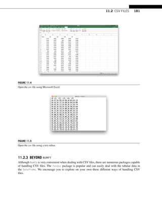
![182 CHAPTER 11 READING AND WRITING DATA
11.3 PICKLE FILES
This section will introduce another way to store the data to the disk, namely pickle. We have talked
about saving data into text files or CSV files, but in certain cases, we want to store dictionaries, tuples,
lists, or any other data type to the disk and use them later or send them to colleagues. This is where
pickle comes in; it can serialize objects so that they can be saved into a file and loaded again later.
Pickle can be used to serialize Python object structures, which refers to the process of converting
an object in the memory to a byte stream that can be stored as a binary file on disk. When we load it
back to a Python program, this binary file can be deserialized back to a Python object.
11.3.1 WRITING TO A PICKLE FILE
TRY IT! Create a dictionary and save it to a pickle file on a disk. To use a pickle, we need to
import the module first.
In [1]: import pickle
In [2]: dict_a = {A:0, B:1, C:2}
pickle.dump(dict_a, open(test.pkl, wb))
To use pickle to serialize an object, we use the pickle.dump function which takes two arguments:
the first one is the object, and the second argument is a file object returned by the open function. Note
that the mode of the open function is wb which indicates it is writing to a binary file.
11.3.2 READING A PICKLE FILE
Next, we load the pickle file we just saved on the disk back using the pickle.load function.
In [3]: my_dict = pickle.load(open(./test.pkl, rb))
my_dict
Out[3]: {A: 0, B: 1, C: 2}
We can see the loading of a pickle file is very similar to the saving process, but here the mode of the
open function is rb, which indicates it is reading the binary file. This function deserializes the binary
file back to the original object, which in this case is a dictionary. This is also one of the reason that the
pickle format is popular; it is very easy to store and load a Python data structure without adding extra
code to change it.
11.3.3 READING IN PYTHON 2 PICKLE FILE
Sometimes, you may need to open a pickle file from some colleague who generated it using Python
2 instead of Python 3. You can either unpickle it using Python 2, or use Python 3 with the encod-
ing=latin1 in the pickle.load function.](https://image.slidesharecdn.com/pythonprogrammingandnumericalmethodsaguideforengineersand-231017183839-0fbc5295/85/Python_Programming_and_Numerical_Methods_A_Guide_for_Engineers_and-pdf-194-320.jpg)
![11.4 JSON FILES 183
infile = open(filename,rb)
new_dict = pickle.load(infile, encoding=latin1)
WARNING! One drawback of pickle files is that they are not in a universal file format, which
means that it is not easy for other programming languages to use it. TXT and CSV files can be
easily shared with other colleagues who are not using Python, and they can open them using R,
Matlab®, Java, and so on. But pickle files are specially designed for Python and the data is not
designed to work with other programming languages.
11.4 JSON FILES
JSON is another format we are introducing. It stands for JavaScript Object Notation. A JSON file
usually ends with the extension “.json”. Unlike pickle, which is Python dependent, JSON is a language-
independent data format, making it attractive to use. In addition, it usually takes up less space on the
disk, and manipulating a JSON file is faster compared to pickle; search online for more detail regarding
the advantages and disadvantages of using JSON versus pickle. Thus, it is a good practice to store your
data using JSON. This section briefly explores how to handle JSON files in Python.
11.4.1 JSON FORMAT
Text in JSON is represented using quoted strings that contain value in key-value pairs within {}; the
structure should appear very similar as it is nearly identical to the dictionary using in Python. For
example,
{
school: UC Berkeley,
address: {
city: Berkeley,
state: California,
postal: 94720
},
list:[
student 1,
student 2,
student 3
]
}](https://image.slidesharecdn.com/pythonprogrammingandnumericalmethodsaguideforengineersand-231017183839-0fbc5295/85/Python_Programming_and_Numerical_Methods_A_Guide_for_Engineers_and-pdf-195-320.jpg)
![184 CHAPTER 11 READING AND WRITING DATA
11.4.2 WRITING A JSON FILE
The easiest way to handle JSON in Python is to use the json library. There are several other libraries
that are available, such as simplejson, jyson, etc. This section will be limited to using json, which is
natively supported by Python to enable you to write and load JSON files.
TRY IT! Create a dictionary and save it to a JSON file on the disk. We need to import the pickle
module first.
In [1]: import json
In [2]: school = {
school: UC Berkeley,
address: {
city: Berkeley,
state: California,
postal: 94720
},
list:[
student 1,
student 2,
student 3
],
array:[1, 2, 3]
}
json.dump(school, open(school.json, w))
To serialize an object using JSON, we use the json.dump function which takes two arguments: the
first one is the object, and the second argument is a file object returned by the open function. Note that
the mode of the open function is w, indicating that it is a “write” file.
11.4.3 READING A JSON FILE
Now we load the JSON file just saved on the disk after using the json.load function.
In [3]: my_school = json.load(open(./school.json, r))
my_school
We can see the use of json is actually very similar to pickle in the last section. JSON supports
strings and numbers, as well as nested lists, tuples, and objects. We suggest exploring these different
options on your own.](https://image.slidesharecdn.com/pythonprogrammingandnumericalmethodsaguideforengineersand-231017183839-0fbc5295/85/Python_Programming_and_Numerical_Methods_A_Guide_for_Engineers_and-pdf-196-320.jpg)
![11.5 HDF5 FILES 185
11.5 HDF5 FILES
Scientific computing often needs to store large amounts of data with quick access; the file formats we
introduced earlier are not applicable. To store large amounts of data, HDF5 (Hierarchical Data Format)
is the solution. It is a powerful binary data format with no limit on the file size. It provides parallel IO
(input/output) and carries out a bunch of low-level optimizations “under the hood” to speed up the
queries and minimize the storage requirements.
An HDF5 file saves two types of objects: datasets, which are array-like collections of data (like
NumPy arrays), and groups, which are folder-like containers that hold datasets and other groups. There
are also attributes that can be associated with the datasets and groups to describe some properties. The
so called hierarchical in HDF5 refers to the fact that the data can be saved like a file system, with
folder-like structures, such as folder, subfolder (in HDF5, it is called group, subgroup). Groups operate
like dictionaries with the keys and values: keys are names of the groups, and values are the subgroups
or datasets.
In order to use read/write HDF5 in Python, there are some packages or wrappers that serve this
purpose. The most common two packages are PyTables2 and h5py.3 We will only introduce the h5py
here. You can install h5py by using conda (refer back to Chapter 1 if you need a refresher).
Once h5py is installed, follow the Quick Start Guide in h5py documentation.4 For your information,
presented below is one example to demonstrate how to create and read an HDF5 file. We will import
the NumPy and h5py first.
In [1]: import numpy as np
import h5py
EXAMPLE: Assume we have deployed instruments to monitor the accelerations and GPS
location in San Francisco Bay Area, California. We have deployed two accelerometers at Berkeley
and Oakland, as well as one GPS station in San Francisco. They record data at different sampling
rates, with the accelerometer at Berkeley sampling the data every 0.04 s, and the sensor in Oakland
at every 0.01 s. The GPS samples the location every 60 s in San Francisco. We want to store the
two types of data into an HDF5, as well as some attributes to indicate where the data has been
recorded, the start time of the recording, station name, and the sampling interval.
In [2]: # Generate random data for recording
acc_1 = np.random.random(1000)
station_number_1 = 1
# unix timestamp
start_time_1 = 1542000276
# time interval for recording
dt_1 = 0.04
2 https://www.pytables.org.
3 https://www.h5py.org.
4 http://docs.h5py.org/en/latest/quick.html.](https://image.slidesharecdn.com/pythonprogrammingandnumericalmethodsaguideforengineersand-231017183839-0fbc5295/85/Python_Programming_and_Numerical_Methods_A_Guide_for_Engineers_and-pdf-197-320.jpg)
![186 CHAPTER 11 READING AND WRITING DATA
location_1 = Berkeley
acc_2 = np.random.random(500)
station_number_2 = 2
start_time_2 = 1542000576
dt_2 = 0.01
location_2 = Oakland
In [3]: hf = h5py.File(station.hdf5, w)
In [4]: hf[/acc/1/data] = acc_1
hf[/acc/1/data].attrs[dt] = dt_1
hf[/acc/1/data].attrs[start_time] = start_time_1
hf[/acc/1/data].attrs[location] = location_1
hf[/acc/2/data] = acc_2
hf[/acc/2/data].attrs[dt] = dt_2
hf[/acc/2/data].attrs[start_time] = start_time_2
hf[/acc/2/data].attrs[location] = location_2
hf[/gps/1/data] = np.random.random(100)
hf[/gps/1/data].attrs[dt] = 60
hf[/gps/1/data].attrs[start_time] = 1542000000
hf[/gps/1/data].attrs[location] = San Francisco
In [5]: hf.close()
The above code shows the core concepts in HDF5: the groups, datasets, and attributes. First, we
created an HDF5 object for writing: station.hdf5. Then we stored the data into two top-level groups:
acc and gps. Both of these top-levels groups contain subgroups labeled 1 or 2 to indicate the station
names. Each station will contain the next level subgroup, i.e., the data, which is used to store the array
data we collected. Next, we add attributes to the groups or the data. In this case, we have added the
dt, start_time, and location as the attributes to the datasets stored here. You can see that it is quite
similar to folder-like structure, with data acc_1 saved at /acc/1/data. Last, we close the file object.
Saving data in HDF5 is easy. We can also use the function create_dataset and create_group as
shown in the quick start.5
11.5.1 READING AN HDF5 FILE
Now suppose you send the station.hdf5 to a colleague, who wants to get access to the data. Here is
how he/she will do it.
5 http://docs.h5py.org/en/latest/quick.html.](https://image.slidesharecdn.com/pythonprogrammingandnumericalmethodsaguideforengineersand-231017183839-0fbc5295/85/Python_Programming_and_Numerical_Methods_A_Guide_for_Engineers_and-pdf-198-320.jpg)
![11.6 SUMMARY AND PROBLEMS 187
In [6]: hf_in = h5py.File(station.hdf5, r)
In [7]: list(hf_in.keys())
Out[7]: [acc, gps]
In [8]: acc = hf_in[acc]
In [9]: list(acc.keys())
Out[9]: [1, 2]
In [10]: data_1 = hf_in[acc/1/data]
In [11]: data_1.value[:10]
Out[11]: array([0.41820889, 0.89832446, 0.40229251, 0.41287538,
0.16173359, 0.75855904, 0.89288185, 0.82944522,
0.84228139, 0.50365515])
In [12]: list(data_1.attrs)
Out[12]: [dt, start_time, location]
In [13]: data_1.attrs[dt]
Out[13]: 0.04
In [14]: data_1.attrs[location]
Out[14]: Berkeley
Reading an HDF5 turns out to be easy as well using h5py. After we read in the HDF5 to hf_in,
we can see what groups are in the HDF5 using the keys function. Then we can get access to the group
members and see what is contained in the subgroups as the hf_in[acc], or directly specify the path
to the datasets as hf_in[acc/1/data] and get the array data. Remember that the attributes associated
with the data can also be accessed as a dictionary.
11.6 SUMMARY AND PROBLEMS
11.6.1 SUMMARY
1. Data must often be stored to a disk for a later Python session or for reading by other programs.
2. Data created by other programs may have to be read by Python.
3. Python has functions to read and write data in several standard forms: TXT, CSV, pickle, and HDF5.](https://image.slidesharecdn.com/pythonprogrammingandnumericalmethodsaguideforengineersand-231017183839-0fbc5295/85/Python_Programming_and_Numerical_Methods_A_Guide_for_Engineers_and-pdf-199-320.jpg)
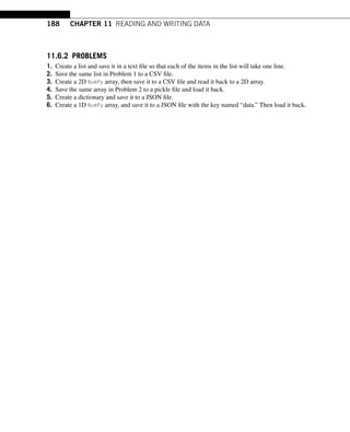
![12
VISUALIZATION AND PLOTTING
12.1 2D Plotting............................................................................................................ 189
12.2 3D Plotting............................................................................................................ 199
12.3 Working With Maps ................................................................................................. 205
12.4 Animations and Movies............................................................................................. 212
12.5 Summary and Problems ............................................................................................ 215
12.5.1 Summary............................................................................................ 215
12.5.2 Problems ............................................................................................ 215
12.1 2D PLOTTING
In Python, the matplotlib is the most important package when plotting data. View the matplotlib
gallery1 to get a sense of what can be done. Usually, the first thing you should do is to import the
matplotlib package. In Jupyter notebook, we can show the figure directly within the notebook and
also have the interactive operations like pan, zoom in/out, and so on using the magic command –
%matplotlib notebook. Below are some examples.
In [1]: import numpy as np
import matplotlib.pyplot as plt
%matplotlib notebook
The basic plotting function is plot(x,y). The plot function takes in two lists/arrays, x and y, and
produces a visual display of the respective points in x and y.
TRY IT! Given the lists x = [0, 1, 2, 3] and y = [0, 1, 4, 9], use the plot function to
produce a plot of x versus y.
In [2]: x = [0, 1, 2, 3]
y = [0, 1, 4, 9]
plt.plot(x, y)
plt.show()
1 https://matplotlib.org/gallery/index.html#gallery.](https://image.slidesharecdn.com/pythonprogrammingandnumericalmethodsaguideforengineersand-231017183839-0fbc5295/85/Python_Programming_and_Numerical_Methods_A_Guide_for_Engineers_and-pdf-201-320.jpg)
![190 CHAPTER 12 VISUALIZATION AND PLOTTING
FIGURE 12.1
Plot of x versus y.
Note in Fig. 12.1 that by default, the plot function connects each point with a blue line. To make
the function look smooth, you can use finer discretization points. The plt.plot function did the main
job to plot the figure, and plt.show() is telling Python that we are done plotting and asks to show
the figure. The buttons beneath the plot allow you to move the line, zoom in or out, or save the figure.
Note that before you plot Fig. 12.2, you need to turn off the interactive plot by pressing the stop
interaction button on the top right of the figure, otherwise, the next figure will be plotted in the same
frame, or use the magic function %matplotlib inline to turn off the interactive features.
TRY IT! Make a plot of the function f (x) = x2 for −5 ≤ x ≤ 5.
In [3]: %matplotlib inline
In [4]: x = np.linspace(-5,5, 100)
plt.plot(x, x**2)
plt.show()](https://image.slidesharecdn.com/pythonprogrammingandnumericalmethodsaguideforengineersand-231017183839-0fbc5295/85/Python_Programming_and_Numerical_Methods_A_Guide_for_Engineers_and-pdf-202-320.jpg)
![12.1 2D PLOTTING 191
FIGURE 12.2
Plot of the function f (x) = x2 for −5 ≤ x ≤ 5.
To change the marker or line, add a third input argument into plot, which is a string that specifies
the color and line style to be used in the plot. For example, plot(x,y,ro) will plot the elements of
x against the elements of y using red, r, circles, o. The possible specifications are shown below in
the table (see also Fig. 12.3).
Symbol Description Symbol Description
b blue T T
g green s square
r red d diamond
c cyan v triangle (down)
m magenta ˆ triangle (up)
y yellow triangle (left)
k black triangle (right)
w white p pentagram
. point h hexagram
o circle - solid
x x-mark : dotted
+ plus -. dashed–dotted
* star - dashed
TRY IT! Make a plot of the function f (x) = x2 for −5 ≤ x ≤ 5 using a dashed green line.
In [5]: x = np.linspace(-5,5, 100)
plt.plot(x, x**2, g-)
plt.show()](https://image.slidesharecdn.com/pythonprogrammingandnumericalmethodsaguideforengineersand-231017183839-0fbc5295/85/Python_Programming_and_Numerical_Methods_A_Guide_for_Engineers_and-pdf-203-320.jpg)
![192 CHAPTER 12 VISUALIZATION AND PLOTTING
FIGURE 12.3
Plot of the function f (x) = x2 for −5 ≤ x ≤ 5 using dashed line.
Before the plt.show() statement, you can add in and plot more datasets within one figure (see also
Fig. 12.4).
TRY IT! Make a plot of the function f (x) = x2 and g(x) = x3 for −5 ≤ x ≤ 5. Use different
colors and markers for each function.
In [6]: x = np.linspace(-5,5,20)
plt.plot(x, x**2, ko)
plt.plot(x, x**3, r*)
plt.show()
FIGURE 12.4
Using different colors and markers.
It is customary in engineering and science to always provide your plot with both title and axis labels
so that people know what your plot is about. Sometimes you want to change the size of the figure as
well. You can add a title to your plot using the title function, which takes as input a string and puts](https://image.slidesharecdn.com/pythonprogrammingandnumericalmethodsaguideforengineersand-231017183839-0fbc5295/85/Python_Programming_and_Numerical_Methods_A_Guide_for_Engineers_and-pdf-204-320.jpg)
![12.1 2D PLOTTING 193
that string as the title of the plot. The functions xlabel and ylabel work in the same way to name your
axis labels. To change the size of the figure, create a figure object and resize it. Note that every time
we call plt.figure function, we create a new figure object and draw on it.
TRY IT! Add a title and axis labels to the previous plot. Make the figure larger so that it is 10
inches wide and 6 inches high.
In [7]: plt.figure(figsize = (10,6))
x = np.linspace(-5,5,20)
plt.plot(x, x**2, ko)
plt.plot(x, x**3, r*)
plt.title(fPlot of Various Polynomials from {x[0]} to
{x[-1]})
plt.xlabel(X axis, fontsize = 18)
plt.ylabel(Y axis, fontsize = 18)
plt.show()
FIGURE 12.5
Adding title and axis labels to a figure.
As demonstrated in Fig. 12.5, we can change any part of the figure, such as the x and y axis label
size by specifying a fontsize argument in the plt.xlabel function. There are some predefined styles
that automatically change the style. Here is the list of the styles.
In [8]: print(plt.style.available)
[seaborn-dark, seaborn-darkgrid, seaborn-ticks,
fivethirtyeight, seaborn-whitegrid, classic,
_classic_test, fast, seaborn-talk,
seaborn-dark-palette, seaborn-bright,
seaborn-pastel, grayscale, seaborn-notebook,](https://image.slidesharecdn.com/pythonprogrammingandnumericalmethodsaguideforengineersand-231017183839-0fbc5295/85/Python_Programming_and_Numerical_Methods_A_Guide_for_Engineers_and-pdf-205-320.jpg)
![194 CHAPTER 12 VISUALIZATION AND PLOTTING
ggplot, seaborn-colorblind, seaborn-muted,
seaborn’, Solarize_Light2, seaborn-paper,
bmh, tableau-colorblind10, seaborn-white,
dark_background, seaborn-poster, seaborn-deep]
One of my favorite predefined styles is the seaborn style; we can change it using the plt.style.use
function. If we change it to seaborn-poster, it will make everything bigger (see also Fig. 12.6).
In [9]: plt.style.use(seaborn-poster)
In [10]: plt.figure(figsize = (10,6))
x = np.linspace(-5,5,20)
plt.plot(x, x**2, ko)
plt.plot(x, x**3, r*)
plt.title(fPlot of Various Polynomials from {x[0]} to
{x[-1]})
plt.xlabel(X axis)
plt.ylabel(Y axis)
plt.show()
FIGURE 12.6
Using seaborn-poster style.
You can create a legend for your plot by using the legend function, by adding the label argument in
the plot function. The legend function also takes argument of loc to indicate where to put the legend;
change it from 0 to 10 and see what happens (see also Fig. 12.7).
In [11]: plt.figure(figsize = (10,6))
x = np.linspace(-5,5,20)
plt.plot(x, x**2, ko, label = quadratic)](https://image.slidesharecdn.com/pythonprogrammingandnumericalmethodsaguideforengineersand-231017183839-0fbc5295/85/Python_Programming_and_Numerical_Methods_A_Guide_for_Engineers_and-pdf-206-320.jpg)
![12.1 2D PLOTTING 195
plt.plot(x, x**3, r*, label = cubic)
plt.title(fPlot of Various Polynomials from {x[0]} to
{x[-1]})
plt.xlabel(X axis)
plt.ylabel(Y axis)
plt.legend(loc = 2)
plt.show()
FIGURE 12.7
Using a legend in the figure.
Finally, you can further customize the appearance of your plots by changing the limits of each axis
using the xlim or ylim function. Using the grid function will turn on the grid of Fig. 12.8.
TRY IT! Change the limits of the plot so that x is visible from −6 to 6, and y is visible from −10
to 10. Turn on the grid.
In [12]: plt.figure(figsize = (10,6))
x = np.linspace(-5,5,100)
plt.plot(x, x**2, ko, label = quadratic)
plt.plot(x, x**3, r*, label = cubic)
plt.title(fPlot of Various Polynomials from {x[0]} to
{x[-1]})
plt.xlabel(X axis)
plt.ylabel(Y axis)
plt.legend(loc = 2)
plt.xlim(-6.6)
plt.ylim(-10,10)
plt.grid()
plt.show()](https://image.slidesharecdn.com/pythonprogrammingandnumericalmethodsaguideforengineersand-231017183839-0fbc5295/85/Python_Programming_and_Numerical_Methods_A_Guide_for_Engineers_and-pdf-207-320.jpg)
![196 CHAPTER 12 VISUALIZATION AND PLOTTING
FIGURE 12.8
Changing limits of the figure and turning on grid.
We can create a table of plots on a single figure using the subplot function. The subplot function
takes three inputs: the number of rows of plots, the number of columns of plots, and designating which
plot all calls to plotting functions should plot. You can move to a different subplot by calling the subplot
again with a different entry for the plot location.
There are several other plotting functions that plot x versus y data. Some of them are scatter,
bar, loglog, semilogx, and semilogy. Function scatter works exactly the same as plot except it
defaults to red circles (i.e., plot(x,y,ro) is equivalent to scatter(x,y)). The bar function plots
bars centered at x with height y. The loglog, semilogx, and semilogy functions plot the data in x and
y, with the x and y axis on a log-scale, the x axis on a log-scale and the y axis on a linear scale, and the
y axis on a log-scale and the x axis on a linear scale, respectively (see also Fig. 12.9).
TRY IT! Given the lists x = np.arange(11) and y = x2, create a 2 × 3 subplot where each subplot
plots x versus y using plot, scatter, bar, loglog, semilogx, and semilogy. Title and label each
plot appropriately. Use a grid, but a legend is not necessary here.
In [13]: x = np.arange(11)
y = x**2
plt.figure(figsize = (14, 8))
plt.subplot(2, 3, 1)
plt.plot(x,y)
plt.title(Plot)
plt.xlabel(X)
plt.ylabel(Y)
plt.grid()
plt.subplot(2, 3, 2)](https://image.slidesharecdn.com/pythonprogrammingandnumericalmethodsaguideforengineersand-231017183839-0fbc5295/85/Python_Programming_and_Numerical_Methods_A_Guide_for_Engineers_and-pdf-208-320.jpg)
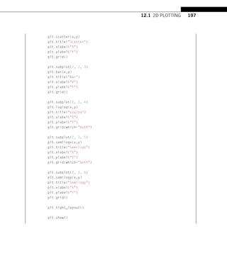
![198 CHAPTER 12 VISUALIZATION AND PLOTTING
FIGURE 12.9
Different type of plots.
We can see that at the end of our plot, we used plt.tight_layout to ensure that the subfigures did
not overlap with each other. Rerun this plot and see the effect without this statement.
Sometimes, you want to save the figures in a specific format, such as pdf, jpeg, png, and so on. You
can do this with the function plt.savefig (see also Fig. 12.10).
In [14]: plt.figure(figsize = (8,6))
plt.plot(x,y)
plt.xlabel(X)
plt.ylabel(Y)
plt.savefig(image.pdf)](https://image.slidesharecdn.com/pythonprogrammingandnumericalmethodsaguideforengineersand-231017183839-0fbc5295/85/Python_Programming_and_Numerical_Methods_A_Guide_for_Engineers_and-pdf-210-320.jpg)
![12.2 3D PLOTTING 199
FIGURE 12.10
Saving a figure.
Finally, there are other functions for plotting data in 2D. The errorbar function plots x versus y
data but with error bars for each element. The polar function plots θ versus r rather than x versus
y. The stem function plots stems at x with height at y. The hist function makes a histogram of a
dataset; boxplot gives a statistical summary of a dataset; and pie makes a pie chart. The usage of these
functions are left for you to explore on your own. Remember to check the examples on the matplotlib
gallery.2
12.2 3D PLOTTING
To plot three-dimensional (3D) figures, first we need to import the mplot3d toolkit, which adds the
simple 3D plotting capabilities to matplotlib.
In [1]: import numpy as np
from mpl_toolkits import mplot3d
import matplotlib.pyplot as plt
plt.style.use(seaborn-poster)
Once we have imported the mplot3d toolkit, we can create 3D axes and add data to the axes. Let us
first create 3D axes (see also Fig. 12.11).
2 https://matplotlib.org/gallery/index.html#gallery.](https://image.slidesharecdn.com/pythonprogrammingandnumericalmethodsaguideforengineersand-231017183839-0fbc5295/85/Python_Programming_and_Numerical_Methods_A_Guide_for_Engineers_and-pdf-211-320.jpg)
![200 CHAPTER 12 VISUALIZATION AND PLOTTING
In [2]: fig = plt.figure(figsize = (10,10))
ax = plt.axes(projection=3d)
plt.show()
FIGURE 12.11
3D axes.
The ax = plt.axes(projection=3d) created a 3D-axes object. To add data to it, use plot3D
function. It is possible to change the title, set the x,y,z labels for the plot as well.
TRY IT! Consider the parameterized dataset: t is a vector from 0 to 10π with a step π/50,
x = sin(t), and y = cos(t). Make a 3D plot of the (x,y,t) dataset using plot3. Turn on the grid,
make the axis equal, and add axis labels and a title. Activate the interactive plot using %matplotlib
notebook so that you can move and rotate the figure as well.
In [3]: %matplotlib notebook
In [4]: fig = plt.figure(figsize = (8,8))
ax = plt.axes(projection=3d)
ax.grid()
t = np.arange(0, 10*np.pi, np.pi/50)
x = np.sin(t)
y = np.cos(t)](https://image.slidesharecdn.com/pythonprogrammingandnumericalmethodsaguideforengineersand-231017183839-0fbc5295/85/Python_Programming_and_Numerical_Methods_A_Guide_for_Engineers_and-pdf-212-320.jpg)
![12.2 3D PLOTTING 201
ax.plot3D(x, y, t)
ax.set_title(3D Parametric Plot)
# Set axes label
ax.set_xlabel(x, labelpad=20)
ax.set_ylabel(y, labelpad=20)
ax.set_zlabel(t, labelpad=20)
plt.show()
See the interactive examples in the notebook.
Try to rotate the above figure to get a 3D view of the plot. You may notice that we also set the
labelpad=20 to the 3-axis labels, which will make it so that the label does not overlap with the tick
texts.
We can also plot a 3D scatter plot using the scatter function (see also Fig. 12.12).
TRY IT! Make a 3D scatter plot with randomly generated 50 data points for x, y, and z. Set the
point color as red and size of the point as 50.
In [5]: # Turn off the interactive plot
%matplotlib inline
In [6]: x = np.random.random(50)
y = np.random.random(50)
z = np.random.random(50)
fig = plt.figure(figsize = (10,10))
ax = plt.axes(projection=3d)
ax.grid()
ax.scatter(x, y, z, c = r, s = 50)
ax.set_title(3D Scatter Plot)
# Set axes label
ax.set_xlabel(x, labelpad=20)
ax.set_ylabel(y, labelpad=20)
ax.set_zlabel(z, labelpad=20)
plt.show()](https://image.slidesharecdn.com/pythonprogrammingandnumericalmethodsaguideforengineersand-231017183839-0fbc5295/85/Python_Programming_and_Numerical_Methods_A_Guide_for_Engineers_and-pdf-213-320.jpg)
![202 CHAPTER 12 VISUALIZATION AND PLOTTING
FIGURE 12.12
3D scatter plot.
When plotting in three dimensions, sometimes it is desirable to use a surface plot rather than a line
plot. In 3D surface plotting, we wish to make a graph of some relationship f (x,y). In surface plotting
all (x,y) pairs must be given. This is not straightforward to do using vectors; therefore, in surface
plotting, the first data structure you must create is called a mesh. Given lists/arrays of x and y values, a
mesh is a listing of all the possible combinations of x and y. In Python, the mesh is given as two arrays
X and Y, where X[i,j] and Y[i,j] that define the possible (x,y) pairs. A third array, Z, can then be
created such that Z[i,j]=f(X[i,j],Y[i,j]). A mesh can be created using the np.meshgrid function
in Python. The meshgrid function has the inputs x and y, which are lists containing the independent
dataset. The output variables X and Y were described earlier.
TRY IT! Create a mesh for x = [1, 2, 3, 4] and y = [3, 4, 5] using the meshgrid function.
In [7]: x = [1, 2, 3, 4]
y = [3, 4, 5]
X, Y = np.meshgrid(x, y)
print(X)
[[1 2 3 4]
[1 2 3 4]](https://image.slidesharecdn.com/pythonprogrammingandnumericalmethodsaguideforengineersand-231017183839-0fbc5295/85/Python_Programming_and_Numerical_Methods_A_Guide_for_Engineers_and-pdf-214-320.jpg)
![12.2 3D PLOTTING 203
[1 2 3 4]]
In [8]: print(Y)
[[3 3 3 3]
[4 4 4 4]
[5 5 5 5]]
In addition, we can plot 3D surfaces in Python: the function to plot 3D surfaces is
plot_surface(X,Y,Z), where X and Y are the output arrays from meshgrid, and Z=f(X,Y) or
Z[i,j]=f(X[i,j],Y[i,j]) (see Fig. 12.13).
TRY IT! Make a plot of the surface f (x,y) = sin(x) · cos(y) for −5 ≤ x ≤ 5,−5 ≤ y ≤ 5 using
the plot_surface function. Take care to use a sufficiently fine discretization in x and y so that the
plot looks smooth.
In [9]: fig = plt.figure(figsize = (12,10))
ax = plt.axes(projection=3d)
x = np.arange(-5, 5.1, 0.2)
y = np.arange(-5, 5.1, 0.2)
X, Y = np.meshgrid(x, y)
Z = np.sin(X)*np.cos(Y)
surf = ax.plot_surface(X, Y, Z, cmap = plt.cm.cividis)
# Set axes label
ax.set_xlabel(x, labelpad=20)
ax.set_ylabel(y, labelpad=20)
ax.set_zlabel(z, labelpad=20)
fig.colorbar(surf, shrink=0.5, aspect=8)
plt.show()](https://image.slidesharecdn.com/pythonprogrammingandnumericalmethodsaguideforengineersand-231017183839-0fbc5295/85/Python_Programming_and_Numerical_Methods_A_Guide_for_Engineers_and-pdf-215-320.jpg)
![204 CHAPTER 12 VISUALIZATION AND PLOTTING
FIGURE 12.13
3D surface plot.
Note that the surface plot shows different colors for different elevations, yellow for higher and
blue for lower (light grey for higher and dark grey for lower in print version); this is because we used
the colormap plt.cm.cividis in the surface plot. You can change to different color schemes for the
surface plot. These are left for you to complete as additional exercises. We also plotted a colorbar to
show the corresponding colors to different values.
We can have subplots of different 3D plots as well (see Fig. 12.14). To do that, use the add_subplot
function from the figure object we created to generate the subplots for 3D cases.
TRY IT! Make a 1 × 2 subplot to plot the above X, Y, Z data in a wireframe plot and a surface
plot.
In [10]: fig = plt.figure(figsize=(12,6))
ax = fig.add_subplot(1, 2, 1, projection=3d)
ax.plot_wireframe(X,Y,Z)
ax.set_title(Wireframe plot)
ax = fig.add_subplot(1, 2, 2, projection=3d)
ax.plot_surface(X,Y,Z)
ax.set_title(Surface plot)](https://image.slidesharecdn.com/pythonprogrammingandnumericalmethodsaguideforengineersand-231017183839-0fbc5295/85/Python_Programming_and_Numerical_Methods_A_Guide_for_Engineers_and-pdf-216-320.jpg)
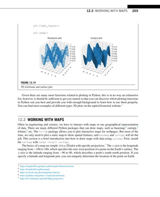
![206 CHAPTER 12 VISUALIZATION AND PLOTTING
The package cartopy has very nice API to interact with matplotlib to plot a map; we only need
to tell the matplotlib to use a specific map projection, and then we can add other map features to the
plot (see also Fig. 12.15).
TRY IT! Plot a world map with cartopy using Plate Carree projection (Google it), and draw the
coastline on the map.
In [1]: import cartopy.crs as ccrs
import matplotlib.pyplot as plt
%matplotlib inline
In [2]: plt.figure(figsize = (12, 8))
ax = plt.axes(projection=ccrs.PlateCarree())
ax.coastlines()
ax.gridlines(draw_labels=True)
plt.show()
FIGURE 12.15
Simple world map.
The above example plotted the map with the Plate Carree projection. In addition, we turned on
the grid lines and drew the labels on the maps. We suggest you check out other cartopy supported
projections.8
The map background we drew above is blank; however, we can easily add a nice map background
in cartopy using stock_img (see also Fig. 12.16).
8 https://scitools.org.uk/cartopy/docs/v0.16/crs/projections.html#cartopy-projections.](https://image.slidesharecdn.com/pythonprogrammingandnumericalmethodsaguideforengineersand-231017183839-0fbc5295/85/Python_Programming_and_Numerical_Methods_A_Guide_for_Engineers_and-pdf-218-320.jpg)
![12.3 WORKING WITH MAPS 207
In [3]: plt.figure(figsize = (12, 8))
ax = plt.axes(projection=ccrs.PlateCarree())
ax.coastlines()
ax.stock_img()
ax.gridlines(draw_labels=True)
plt.show()
FIGURE 12.16
World map with background.
We can zoom in the map to any places on the Earth using the ax.set_extent function, which takes
a list with the first two numbers that are the x-axis limits and the last two numbers are the y-axis limits
(see also Fig. 12.17).
TRY IT! Zoom in the map to the United States.
In [4]: plt.figure(figsize = (10, 5))
ax = plt.axes(projection=ccrs.PlateCarree())
ax.coastlines()
ax.set_extent([-125, -75, 25, 50])
ax.gridlines(draw_labels=True)
plt.show()](https://image.slidesharecdn.com/pythonprogrammingandnumericalmethodsaguideforengineersand-231017183839-0fbc5295/85/Python_Programming_and_Numerical_Methods_A_Guide_for_Engineers_and-pdf-219-320.jpg)
![208 CHAPTER 12 VISUALIZATION AND PLOTTING
FIGURE 12.17
Simple US map.
Did you notice that there are no features added on the map, such as the country boundary, state
boundary, lakes/water, etc.? In cartopy, these features must be specified if we want to add them to our
map (see also Fig. 12.18).
TRY IT! For the map of the United States we made above, add the following features: land,
ocean, states and country borders, lakes, and rivers.
In [5]: import cartopy.feature as cfeature
In [6]: plt.figure(figsize = (10, 5))
ax = plt.axes(projection=ccrs.PlateCarree())
ax.coastlines()
ax.set_extent([-125, -75, 25, 50])
ax.add_feature(cfeature.LAND)
ax.add_feature(cfeature.OCEAN)
ax.add_feature(cfeature.STATES, linestyle=:)
ax.add_feature(cfeature.BORDERS)
ax.add_feature(cfeature.LAKES, alpha=0.5)
ax.add_feature(cfeature.RIVERS)
plt.show()](https://image.slidesharecdn.com/pythonprogrammingandnumericalmethodsaguideforengineersand-231017183839-0fbc5295/85/Python_Programming_and_Numerical_Methods_A_Guide_for_Engineers_and-pdf-220-320.jpg)
![12.3 WORKING WITH MAPS 209
FIGURE 12.18
US map with various features.
It is possible to zoom in further to a smaller area, but we would need to download and use the
high-resolution coastlines and land to have a decent-looking map (see also Fig. 12.19).
TRY IT! Plot the San Francisco Bay Area with the 10 m-resolution coastlines and land. Try to
change one of them to 50 m and see what happens.
In [7]: plt.figure(figsize = (10, 8))
ax = plt.axes(projection=ccrs.PlateCarree())
ax.coastlines(resolution=10m)
ax.set_extent([-122.8, -122, 37.3, 38.3])
# we can add high-resolution land and water
LAND =
cfeature.NaturalEarthFeature(physical, land, 10m,
edgecolor=face,
facecolor=cfeature.COLORS[land],
linewidth=.1)
OCEAN =
cfeature.NaturalEarthFeature(physical,ocean,10m,
edgecolor=face,
facecolor=cfeature.COLORS[water],
linewidth=.1)
ax.add_feature(LAND, zorder=0)
ax.add_feature(OCEAN, zorder=0)](https://image.slidesharecdn.com/pythonprogrammingandnumericalmethodsaguideforengineersand-231017183839-0fbc5295/85/Python_Programming_and_Numerical_Methods_A_Guide_for_Engineers_and-pdf-221-320.jpg)
![210 CHAPTER 12 VISUALIZATION AND PLOTTING
plt.show()
FIGURE 12.19
Bay area map with higher resolution.
In many cases, we want to plot our data onto the map and show the spatial location of different
entities. Data can be added to it in exactly the same way as with normal matplotlib axes. By default,
the coordinate system of any additional data is the same as the coordinate system of the axes we defined
at the beginning of the plot. Let us first try to add some data to the map above (see also Fig. 12.20).
TRY IT! Add the location of UC Berkeley and Stanford University on the Bay Area map above.
In [8]: plt.figure(figsize = (10, 8))
# plot the map related stuff
ax = plt.axes(projection=ccrs.PlateCarree())
ax.coastlines(resolution=10m)
ax.set_extent([-122.8, -122, 37.3, 38.3])
ax.add_feature(LAND, zorder=0)
ax.add_feature(OCEAN, zorder=0)](https://image.slidesharecdn.com/pythonprogrammingandnumericalmethodsaguideforengineersand-231017183839-0fbc5295/85/Python_Programming_and_Numerical_Methods_A_Guide_for_Engineers_and-pdf-222-320.jpg)
![12.3 WORKING WITH MAPS 211
# plot the data related stuff
berkeley_lon, berkeley_lat = -122.2585, 37.8719
stanford_lon, stanford_lat = -122.1661, 37.4241
# plot the two universities as blue dots
ax.plot([berkeley_lon, stanford_lon],
[berkeley_lat, stanford_lat],
color=blue, linewidth=2, marker=o)
# add labels for the two universities
ax.text(berkeley_lon + 0.16, berkeley_lat - 0.02,
UC Berkeley, horizontalalignment=right)
ax.text(stanford_lon + 0.02, stanford_lat - 0.02,
Stanford, horizontalalignment=left)
plt.show()
FIGURE 12.20
Add more entities on the map.](https://image.slidesharecdn.com/pythonprogrammingandnumericalmethodsaguideforengineersand-231017183839-0fbc5295/85/Python_Programming_and_Numerical_Methods_A_Guide_for_Engineers_and-pdf-223-320.jpg)
![212 CHAPTER 12 VISUALIZATION AND PLOTTING
The cartopy package is extremely versatile. The official example is available at the gallery online.9
We suggest exploring this on your own to augment your map-making abilities.
12.4 ANIMATIONS AND MOVIES
An animation is a sequence of still frames, or plots, that are displayed in fast enough succession to
create the illusion of continuous motion. Animations and movies often convey information better than
individual plots. You can create animations in Python by calling a plot function inside of a loop (usually
a for-loop). The main tools for making animations in Python is the matplotlib.animation.Animation
base class, which provides a framework around which the animation functionality is built. See the
example below.
TRY IT! Create an animation of a red circle following a blue sine wave.
In [1]: import numpy as np
import matplotlib.pyplot as plt
import matplotlib.animation as manimation
In [2]: n = 1000
x = np.linspace(0, 6*np.pi, n)
y = np.sin(x)
# Define the meta data for the movie
FFMpegWriter = manimation.writers[ffmpeg]
metadata = dict(title=Movie Test, artist=Matplotlib,
comment=a red circle following a blue sine wave)
writer = FFMpegWriter(fps=15, metadata=metadata)
# Initialize the movie
fig = plt.figure()
# plot the sine wave line
sine_line, = plt.plot(x, y, b)
red_circle, = plt.plot([], [], ro, markersize = 10)
plt.xlabel(x)
plt.ylabel(sin(x))
# Update the frames for the movie
with writer.saving(fig, writer_test.mp4, 100):
9 https://scitools.org.uk/cartopy/docs/latest/gallery/index.html.](https://image.slidesharecdn.com/pythonprogrammingandnumericalmethodsaguideforengineersand-231017183839-0fbc5295/85/Python_Programming_and_Numerical_Methods_A_Guide_for_Engineers_and-pdf-224-320.jpg)
![12.4 ANIMATIONS AND MOVIES 213
for i in range(n):
x0 = x[i]
y0 = y[i]
red_circle.set_data(x0, y0)
writer.grab_frame()
Before we make a movie, it is advised to first follow the next three steps:
• Define the meta data for the movie.
• Decide what in the background does not need changing.
• Decide which objects needs changing in each movie frame.
Once these parameters are determined, it is relatively easy to make the movie using Python follow-
ing the next three steps:
• Define the meta data for the movie.
• Initialize the movie background figure.
• Update the frames for the movie.
Using the example above, we can clearly see how the code relates to these three steps.
1. Defining the meta data for the movie
FFMpegWriter = manimation.writers[ffmpeg]
metadata = dict(title=Movie Test, artist=Matplotlib,
comment=a red circle following a blue sine wave)
writer = FFMpegWriter(fps=15, metadata=metadata)
This block of code is telling Python that we want to create a movie using a movie writer
and need to provide the title, artist, and any necessary commentary. In addition, we need to tell](https://image.slidesharecdn.com/pythonprogrammingandnumericalmethodsaguideforengineersand-231017183839-0fbc5295/85/Python_Programming_and_Numerical_Methods_A_Guide_for_Engineers_and-pdf-225-320.jpg)
![214 CHAPTER 12 VISUALIZATION AND PLOTTING
Python the rate of the frames in the movie, that is, fps=15, which means that we want to display
15 consecutive frames within 1 s (fps stands for frames per second).
2. Initializing the movie background figure
fig = plt.figure()
# plot the sine wave line
sine_line, = plt.plot(x, y, b)
red_circle, = plt.plot([], [], ro, markersize = 10)
plt.xlabel(x)
plt.ylabel(sin(x))
First we need to initialize the background figure for the movie. The reason we call it the
background figure is that the graphics we plot here will not change during the movie. In this
example, the sine wave curve will not change. At the same time, we plot an empty red dot (which
will not appear on the figure). It serves as a place holder for the things that will change later in
the movie; this is equivalent to telling Python that we will have a red point and we will update the
location of the point later. In this case, the x and y axes labels will not change, and, therefore, are
plotted them here.
3. Updating the frames for the movie
with writer.saving(fig, writer_test.mp4, 100):
for i in range(n):
x0 = x[i]
y0 = y[i]
red_circle.set_data(x0, y0)
writer.grab_frame()
This block of code specifies the name of the output file, format, and resolution of the figure
(dpi – dots per inch). In this case, we want the output file to have a name writer_test with the
format mp4, and we want a dpi of 100 for this figure. Next we code the core part of the movie:
repeated updating of the figure, i.e., to create the “motion.” We use a for-loop to update the figure,
and in each loop, we change the location (x, y location) of the red circle. The writer.grab_frame
function will capture this change in each frame and display it based on the fps we set.
This is how to make a simple movie.
Numerous examples on how to make a movie are available in matplotlib movie tutorial.10 Run
through some of the examples to get a better understanding of how to make movies in Python.
10 https://matplotlib.org/api/animation_api.html.](https://image.slidesharecdn.com/pythonprogrammingandnumericalmethodsaguideforengineersand-231017183839-0fbc5295/85/Python_Programming_and_Numerical_Methods_A_Guide_for_Engineers_and-pdf-226-320.jpg)
![12.5 SUMMARY AND PROBLEMS 215
12.5 SUMMARY AND PROBLEMS
12.5.1 SUMMARY
1. Visualizing data is an essential tool in engineering and science applications.
2. Python has many different packages of plotting tools that can be used to visualize data.
3. Two- and three-dimensional plots and maps are usually used in engineering and science to commu-
nicate research results.
4. Videos are a sequence of static images that are displayed at a certain speed.
12.5.2 PROBLEMS
1. A cycloid is the curve traced by a point located on the edge of a wheel rolling along a flat surface.
The (x,y) coordinates of a cycloid generated from a wheel with radius, r, can be described by the
parametric equations:
x = r(φ − sinφ),
y = r(1 − cosφ),
where φ is the number of radians that the wheel has rolled through.
Generate a plot of the cycloid for 0 ≤ φ ≤ 2π using 1000 increments and r = 3. Give your plot a
title and labels. Turn on the grid and modify the axis limits to make the plot neat and attractive.
2. Consider the following function:
y(x) =
100(1 − 0.01x2)2 + 0.02x2
(1 − x2)2 + 0.1x2
.
Generate a 2 × 2 subplot of y(x) for 0 ≤ x ≤ 100 using plot, semilogx, semilogy, and loglog.
Use a fine enough discretization in x to make the plot appear smooth. Give each plot axis labels
and a title. Turn on the grid. Which plot seems to convey the most information?.
3. Plot the functions y1(x) = 3 + exp(−x)sin(6x) and y2(x) = 4 + exp(−x)cos(6x) for 0 ≤ x ≤ 5
on a single axis. Give the plot axis labels, a title, and a legend.
4. Generate 1000 normally distributed random numbers using the np.random.randn function. Look
up the help for the plt.hist function. Use the plt.hist function to plot a histogram of the
randomly generated numbers. Use the plt.hist function to distribute the randomly generated
numbers into 10 bins. Create a bar graph of the output using the plt.bar function. It should look
very similar to the plot produced by plt.hist.
Do you think that the np.random.randn function is a good approximation of a normally distributed
number?
5. Let the number of students with A’s, B’s, C’s, D’s, and F’s be contained in the list grade_dist =
[42, 85, 67, 20, 5]. Use the plt.pie function to generate a pie chart of grade_dist. Put a title
and legend on the pie chart.
6. Let −4 ≤ x ≤ 4,−3 ≤ y ≤ 3, and z(x,y) = xy(x2−y2)
x2+y2 . Create arrays x and y with 100 evenly
spaced points over the interval. Create meshgrids X and Y for x and y using the meshgrid func-](https://image.slidesharecdn.com/pythonprogrammingandnumericalmethodsaguideforengineersand-231017183839-0fbc5295/85/Python_Programming_and_Numerical_Methods_A_Guide_for_Engineers_and-pdf-227-320.jpg)
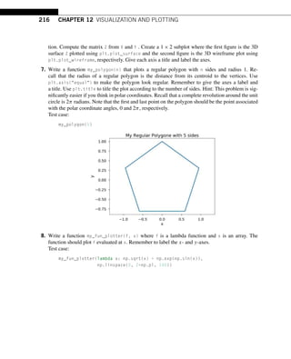
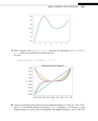
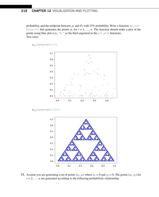
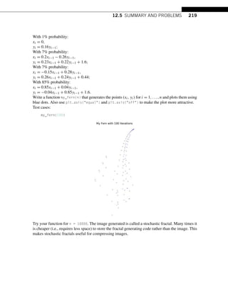
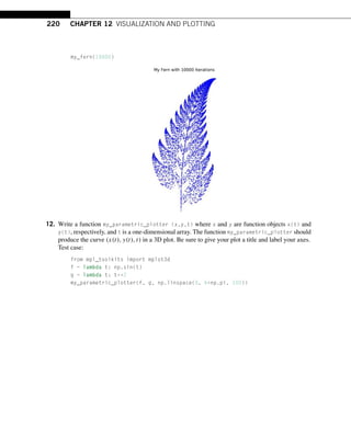
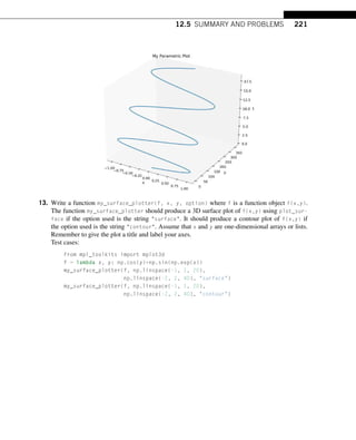
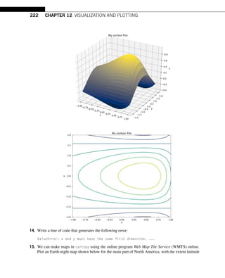

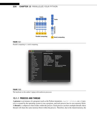
![13.2 MULTIPROCESSING 227
variables or objects for multiple threads in a process are all shared. If you change one variable in one
thread, it will change for all the other threads. This is not the case for different processes. If you change
one variable in one process, it will not change that variable in other processes. Process and thread both
have advantages or disadvantages, and can be used in different tasks to maximize the benefits of each.
13.1.2 PYTHON’S GIL PROBLEM
Python was designed before the multicore processors were available on personal computers (this shows
you how old the language is). It contains an inherent limitation called Global Interpreter Lock (GIL),
whereby only one native thread can run at any time, i.e., it prevents multiple threads from running
simultaneously. Even though there are workarounds in Python to do multithreading, only multipro-
cessing library will be covered below.
13.1.3 DISADVANTAGES OF USING PARALLEL COMPUTING
There are disadvantages when using parallel computing: the code becomes more complicated because
of the overheads required to launch and maintain new processes. Thus, if your task is small, using
parallel computing will actually take longer since it takes time for the system to initialize new processes
and maintain them.
13.2 MULTIPROCESSING
The multiprocessing library, Python’s standard library to support its parallel computing using pro-
cesses, has many different features that are too numerous to discuss herein. We suggest you check out
the official documentation.1 Here, we are introducing only the basics to get you started with parallel
computing. Let us start by importing the library and printing out the total number of CPUs on your
machine that can be used for parallel computing.
In [1]: import multiprocessing as mp
In [2]: print(fNumber of cpu: {mp.cpu_count()})
Number of cpu: 12
The example below shows you how to use multiple cores in one machine to reduce the execution
time.
1 https://docs.python.org/3/library/multiprocessing.html.](https://image.slidesharecdn.com/pythonprogrammingandnumericalmethodsaguideforengineersand-231017183839-0fbc5295/85/Python_Programming_and_Numerical_Methods_A_Guide_for_Engineers_and-pdf-238-320.jpg)
![228 CHAPTER 13 PARALLELIZE YOUR PYTHON
EXAMPLE: Generate 10,000,000 random numbers between 0 and 10, and square them. Store
the results in a list.
Serial version
In [3]: import numpy as np
import time
def random_square(seed):
np.random.seed(seed)
random_num = np.random.randint(0, 10)
return random_num**2
In [4]: t0 = time.time()
results = []
for i in range(10000000):
results.append(random_square(i))
t1 = time.time()
print(fExecution time {t1 - t0} s)
Execution time 38.20956087112427 s
Parallel version
The simplest way to do parallel computing using the multiprocessing is to use the pool class. There
are four common methods in this class that are used often: apply, map, apply_async, and map_async.
Look at the documentation for the differences between them for your own edification. We will only use
the map function in parallel with the above example. The map(func, iterable) function takes in two
arguments. Apply the function func to each element in the iterable and then collect the results.
In [5]: t0 = time.time()
n_cpu = mp.cpu_count()
pool = mp.Pool(processes=n_cpu)
results = [pool.map(random_square, range(10000000))]
t1 = time.time()
print(fExecution time {t1 - t0} s)
Execution time 7.130078077316284 s
Using the above parallel version of the code reduced the run time from ~38 s to ~7 s. This is a big
gain in speed, especially if we were running a code that demanded a lot of computation.
The pool.apply function is similar except that it can accept more arguments. The pool.map and
pool.apply will lock the main program until all the processes are finished, which is quite useful if we](https://image.slidesharecdn.com/pythonprogrammingandnumericalmethodsaguideforengineersand-231017183839-0fbc5295/85/Python_Programming_and_Numerical_Methods_A_Guide_for_Engineers_and-pdf-239-320.jpg)
![13.2 MULTIPROCESSING 229
want to obtain results in a particular order for some applications. In contrast, if we do not need the
results in a particular order, we can also use pool.apply_async or pool.map_async, which will submit
all processes at once and retrieve the results as soon as they are finished. Check online to learn more.
13.2.1 VISUALIZE THE EXECUTION TIME
Let us visualize the execution time changes versus the number of data points using both the serial and
parallel version. You will see that until a certain point, it is better to use the serial version.
In [6]: import matplotlib.pyplot as plt
plt.style.use(seaborn-poster)
%matplotlib inline
def serial(n):
t0 = time.time()
results = []
for i in range(n):
results.append(random_square(i))
t1 = time.time()
exec_time = t1 - t0
return exec_time
def parallel(n):
t0 = time.time()
n_cpu = mp.cpu_count()
pool = mp.Pool(processes=n_cpu)
results = [pool.map(random_square, range(n))]
t1 = time.time()
exec_time = t1 - t0
return exec_time
In [7]: n_run = np.logspace(1, 7, num = 7)
t_serial = [serial(int(n)) for n in n_run]
t_parallel = [parallel(int(n)) for n in n_run]
In [8]: plt.figure(figsize = (10, 6))
plt.plot(n_run, t_serial, -o, label = serial)
plt.plot(n_run, t_parallel, -o, label = parallel)
plt.loglog()
plt.legend()
plt.ylabel(Execution time (s))](https://image.slidesharecdn.com/pythonprogrammingandnumericalmethodsaguideforengineersand-231017183839-0fbc5295/85/Python_Programming_and_Numerical_Methods_A_Guide_for_Engineers_and-pdf-240-320.jpg)
![230 CHAPTER 13 PARALLELIZE YOUR PYTHON
plt.xlabel(Number of random points)
plt.show()
As shown in the figure, when the number of data points is small (below 10000), the execution
time for the serial version is faster due to the overhead of the parallel version necessary to launch and
maintain the new processes. After that point, the parallel version would be a better choice. For example,
when we have 107 data points, the parallel version uses less than 10 s to finish the task while the serial
version takes roughly 50 s.
13.3 USING JOBLIB
Python also has other third party packages that can make the parallel computing easier, especially for
some daily tasks, e.g., package joblib2 provides a simple way to perform parallel computing (and has
many other usages as well).
First, install this package by running pip install joblib; then run the previous example using
this new package.
In [1]: from joblib import Parallel, delayed
import numpy as np
def random_square(seed):
np.random.seed(seed)
random_num = np.random.randint(0, 10)
return random_num**2
2 https://joblib.readthedocs.io/en/latest/index.html.](https://image.slidesharecdn.com/pythonprogrammingandnumericalmethodsaguideforengineersand-231017183839-0fbc5295/85/Python_Programming_and_Numerical_Methods_A_Guide_for_Engineers_and-pdf-241-320.jpg)
![13.4 SUMMARY AND PROBLEMS 231
In [2]: results = Parallel(n_jobs=8)
(delayed(random_square)(i) for i in range(1000000))
Note that the parallel part of the code becomes one line by using the joblib package, which is
very convenient. Parallel is a helper class that essentially provides a convenient interface for the
multiprocessing module we saw earlier. The delayed function is used to capture the arguments of
the target function, which in this case is the random_square. We ran the above code with eight CPUs.
If you want to use all the computational power on your machine, you can use all available CPUs on
your machine by setting n_jobs=-1. If you set it to -2, all CPUs but one will be used. In addition, turn
on the verbose argument if you want to output the status messages.
In [3]: results = Parallel(n_jobs=-1, verbose=1)
(delayed(random_square)(i) for i in range(1000000))
[Parallel(n_jobs=-1)]: Using backend LokyBackend with 12
concurrent workers.
[Parallel(n_jobs=-1)]: Done 60 tasks | elapsed: 0.1s
[Parallel(n_jobs=-1)]: Done 176056 tasks | elapsed: 3.0s
[Parallel(n_jobs=-1)]: Done 787056 tasks | elapsed: 12.4s
[Parallel(n_jobs=-1)]: Done 1000000 out of 1000000 |
elapsed: 15.5s finished
There are multiple backends in joblib, which means using different ways to do the parallel computing.
If you set the backend as multiprocessing, i.e., under the hood, it creates a multiprocessing pool that
uses separate Python worker processes to execute tasks concurrently on separate CPUs.
In [4]: results =
Parallel(n_jobs=-1, backend=multiprocessing, verbose=1)
(delayed(random_square)(i) for i in range(1000000))
[Parallel(n_jobs=-1)]: Using backend MultiprocessingBackend
with 12 concurrent workers.
[Parallel(n_jobs=-1)]: Done 220 tasks | elapsed: 0.0s
[Parallel(n_jobs=-1)]: Done 457032 tasks | elapsed: 1.9s
[Parallel(n_jobs=-1)]: Done 1000000 out of 1000000 |
elapsed: 3.8s finished
13.4 SUMMARY AND PROBLEMS
13.4.1 SUMMARY
1. Parallel computing can reduce execution time by using multiple cores on your computer.](https://image.slidesharecdn.com/pythonprogrammingandnumericalmethodsaguideforengineersand-231017183839-0fbc5295/85/Python_Programming_and_Numerical_Methods_A_Guide_for_Engineers_and-pdf-242-320.jpg)
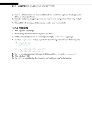
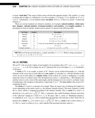
![14.1 BASICS OF LINEAR ALGEBRA 237
TRY IT! Create a row vector and a column vector, and show their shape.
In [1]: import numpy as np
vector_row = np.array([[1, -5, 3, 2, 4]])
vector_column = np.array([[1],[2],[3],[4]])
print(vector_row.shape)
print(vector_column.shape)
(1, 5)
(4, 1)
Note! In Python, the row and column vectors can be tricky. As shown in the example above, in order
to get the 1 row and 4 column or 4 row and 1 column vectors, we had to use a list of a list to specify
it. You can define np.array([1,2,3,4]), but you will soon notice that it does not contain information
about row or column.
TRY IT! Transpose the row vector defined above into a column vector and calculate its L1, L2,
and L∞ norm. Verify that the L∞ norm of a vector is equivalent to the maximum value of the
elements in the vector.
In [2]: from numpy.linalg import norm
new_vector = vector_row.T
print(new_vector)
norm_1 = norm(new_vector, 1)
norm_2 = norm(new_vector, 2)
norm_inf = norm(new_vector, np.inf)
print(L_1 is: %.1f%norm_1)
print(L_2 is: %.1f%norm_2)
print(L_inf is: %.1f%norm_inf)
[[ 1]
[-5]
[ 3]
[ 2]
[ 4]]
L_1 is: 15.0
L_2 is: 7.4
L_inf is: 5.0
Vector addition is defined as the pairwise addition of the elements of the added vectors. For exam-
ple, if v and w are vectors in Rn, then u = v + w is defined as having elements ui = vi + wi.](https://image.slidesharecdn.com/pythonprogrammingandnumericalmethodsaguideforengineersand-231017183839-0fbc5295/85/Python_Programming_and_Numerical_Methods_A_Guide_for_Engineers_and-pdf-246-320.jpg)
![238 CHAPTER 14 LINEAR ALGEBRA AND SYSTEMS OF LINEAR EQUATIONS
Vector multiplication can be defined in several ways depending on the context. Scalar multipli-
cation of a vector is the product of a vector and a scalar (i.e., a number in R). Scalar multiplication is
defined as the product of each element of the vector by the scalar. More specifically, if α is a scalar and
v is a vector, then u = αv is defined as having elements ui = αvi. Note that this is exactly how Python
implements scalar multiplication with a vector.
TRY IT! Show that a(v + w) = av + aw (i.e., scalar multiplication of a vector distributes across
vector addition).
By vector addition, u = v + w is the vector with entries ui = vi + wi. By definition of scalar
multiplication of a vector, x = αu is the vector with elements xi = α(vi + wi). Since α,vi, and
wi are scalars, multiplication distributes and xi = αvi + αwi. Therefore, a(v + w) = av + aw.
The dot-product of two vectors is the sum of the products of the respective elements and is denoted
by ·, and v · w is read “v dot w.” Therefore for v,w ∈ Rn,d = v · w is defined as d =
n
i=1 viwi. The
angle between two vectors, θ, is defined by the formula:
v · w = v2w2 cosθ.
The dot-product is a measure of how similarly directed the two vectors are. For example, the vectors
(1,1) and (2,2) are parallel. If you compute the angle between them using the dot-product, you will
find that θ = 0. If the angle between the vectors is θ = π/2, then the vectors are said to be perpendicular
or orthogonal, and the dot-product is 0.
TRY IT! Compute the angle between the vectors v = [10,9,3] and w = [2,5,12].
In [3]: from numpy import arccos, dot
v = np.array([[10, 9, 3]])
w = np.array([[2, 5, 12]])
theta = arccos(dot(v, w.T)/(norm(v)*norm(w)))
print(theta)
[[0.97992471]]
Finally, the cross-product between two vectors, v and w, is written as v × w. It is defined by
v × w = v2w2 sin(θ)n, where θ is the angle between the v and w (which can be computed
from the dot-product), and n is a vector perpendicular to both v and w with unit length (i.e., its
length is one). The geometric interpretation of the cross-product is a vector perpendicular to both
v and w, with the length equal to the area enclosed by the parallelogram created by the two vec-
tors.](https://image.slidesharecdn.com/pythonprogrammingandnumericalmethodsaguideforengineersand-231017183839-0fbc5295/85/Python_Programming_and_Numerical_Methods_A_Guide_for_Engineers_and-pdf-247-320.jpg)
![14.1 BASICS OF LINEAR ALGEBRA 239
TRY IT! Given the vectors v = [0,2,0] and w = [3,0,0], use the NumPy function cross to com-
pute the cross-product of v and w.
In [4]: v = np.array([[0, 2, 0]])
w = np.array([[3, 0, 0]])
print(np.cross(v, w))
[[ 0 0 -6]]
Assuming that S is a set in which addition and scalar multiplication are defined, a linear combina-
tion of S is defined as
αisi,
where αi is any real number, and si is the ith object in S. Sometimes the αi values are called the
coefficients of si.
Linear combinations can be used to describe numerous things. For example, a grocery bill can be
written
cini, where ci is the cost of item i and ni is the number of items i purchased. Thus, the total
cost is a linear combination of the items purchased.
A set is called linearly independent if no object in the set can be written as a linear combination of
the other objects in the set. For the purposes of this book, we will only consider the linear independence
of a set of vectors. A set of vectors that is not linearly independent is linearly dependent.
TRY IT! Given the row vectors v = [0,3,2], w = [4,1,1], and u = [0,−2,0], write the vector
x = [−8,−1,4] as a linear combination of v, w, and u.
In [5]: v = np.array([[0, 3, 2]])
w = np.array([[4, 1, 1]])
u = np.array([[0, -2, 0]])
x = 3*v-2*w+4*u
print(x)
[[-8 -1 4]]
TRY IT! Determine by inspection whether the following set of vectors is linearly independent:
v = [1,1,0], w = [1,0,0], u = [0,0,1].
Clearly, u is linearly independent from v and w because only u has a nonzero third element.
The vectors v and w are also linearly independent because only v has a nonzero second element.
Therefore, v,w, and u are linearly independent.
14.1.3 MATRICES
An m × n matrix is a rectangular table of numbers consisting of m rows and n columns. The norm of
a matrix can be considered as a particular kind of vector norm. If we treat the m × n elements of M as](https://image.slidesharecdn.com/pythonprogrammingandnumericalmethodsaguideforengineersand-231017183839-0fbc5295/85/Python_Programming_and_Numerical_Methods_A_Guide_for_Engineers_and-pdf-248-320.jpg)
![240 CHAPTER 14 LINEAR ALGEBRA AND SYSTEMS OF LINEAR EQUATIONS
the elements of an mn-dimensional vector, then the p-norm of this vector can be written as
Mp = p
m
i
n
j
|aij |p.
It is possible to calculate the matrix norm using the same norm function in NumPy as that for a
vector.
Matrix addition and scalar multiplication for matrices work the same way as for vectors. However,
matrix multiplication between two matrices, P and Q, is defined when P is an m × p matrix and Q
is a p × n matrix. The result of M = PQ is a matrix M that is m × n. The dimension p is called the
inner matrix dimension, and the inner matrix dimensions must match (i.e., the number of columns
in P and the number of rows in Q must be the same) for matrix multiplication to be defined. The
dimensions m and n are called the outer matrix dimensions. Formally, if P is m × p and Q is p × n,
then M = PQ is defined as
Mij =
p
k=1
PikQkj .
The product of two matrices P and Q in Python is achieved by using the dot method in NumPy.
The transpose of a matrix is a reversal of its rows with its columns. The transpose is denoted by a
superscript, T , such as MT is the transpose of matrix M. In Python, the method T for a NumPy array is
used to get the transpose. For example, if M is a matrix, then M.T is its transpose.
TRY IT!
Let matrices P and Q be [[1,7],[2,3],[5,0]] and [[2,6,3,1],[1,2,3,4]], respectively. Com-
pute the Python matrix product of P and Q. Show that the product of Q and P will produce an
error.
In [6]: P = np.array([[1, 7], [2, 3], [5, 0]])
Q = np.array([[2, 6, 3, 1], [1, 2, 3, 4]])
print(P)
print(Q)
print(np.dot(P, Q))
np.dot(Q, P)
[[1 7]
[2 3]
[5 0]]
[[2 6 3 1]
[1 2 3 4]]
[[ 9 20 24 29]
[ 7 18 15 14]
[10 30 15 5]]](https://image.slidesharecdn.com/pythonprogrammingandnumericalmethodsaguideforengineersand-231017183839-0fbc5295/85/Python_Programming_and_Numerical_Methods_A_Guide_for_Engineers_and-pdf-249-320.jpg)
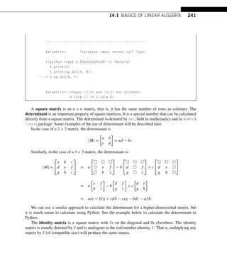
![242 CHAPTER 14 LINEAR ALGEBRA AND SYSTEMS OF LINEAR EQUATIONS
TRY IT!
Find the determinant of matrix M = [[0,2,1,3],[3,2,8,1],[1,0,0,3],[0,3,2,1]]. Use the
np.eye function to produce a 4 × 4 identity matrix, I. Multiply M by I to show that the result is
M.
In [7]: from numpy.linalg import det
M = np.array([[0,2,1,3],
[3,2,8,1],
[1,0,0,3],
[0,3,2,1]])
print(M:n, M)
print(Determinant: %.1f%det(M))
I = np.eye(4)
print(I:n, I)
print(M*I:n, np.dot(M, I))
M:
[[0 2 1 3]
[3 2 8 1]
[1 0 0 3]
[0 3 2 1]]
Determinant: -38.0
I:
[[1. 0. 0. 0.]
[0. 1. 0. 0.]
[0. 0. 1. 0.]
[0. 0. 0. 1.]]
M*I:
[[0. 2. 1. 3.]
[3. 2. 8. 1.]
[1. 0. 0. 3.]
[0. 3. 2. 1.]]
The inverse of a square matrix M is a matrix of the same size, N, such that M · N = I. The inverse
of a matrix is analogous to the inverse of a real number. For example, the inverse of 3 is 1
3 because
(3)(1
3 ) = 1. A matrix is said to be invertible if it has an inverse. The inverse of a matrix is unique,
that is, for an invertible matrix, there is only one inverse for that matrix. If M is a square matrix, its
inverse is denoted by M−1 in mathematics, and it can be computed in Python using the function inv
from NumPy’s linalg package.
For a 2 × 2 matrix, the analytical solution of the matrix inverse is](https://image.slidesharecdn.com/pythonprogrammingandnumericalmethodsaguideforengineersand-231017183839-0fbc5295/85/Python_Programming_and_Numerical_Methods_A_Guide_for_Engineers_and-pdf-251-320.jpg)
![14.1 BASICS OF LINEAR ALGEBRA 243
M−1
=
a b
c d
−1
=
1
|M|
d −b
−c a
.
Calculating the matrix inverse for the analytical solution becomes complicated as the dimension of
the matrix increases. There are many other methods which can make things easier, such as Gaussian
elimination, Newton’s method, eigendecomposition, etc. We will introduce some of these methods
after we learn how to solve a system of linear equations (as the process is essentially the same).
Recall that zero has no inverse for multiplication in the setting of real numbers. Similarly, there are
matrices that do not have inverses. These matrices are called singular. Matrices that do have an inverse
are called nonsingular.
One way to determine if a matrix is singular is by computing its determinant. If the determinant is
0, then the matrix is singular; if not, the matrix is non-singular.
TRY IT! The matrix M (in the previous example) has a nonzero determinant. Compute the inverse
of M. Show that the matrix P = [[0,1,0],[0,0,0],[1,0,1]] has a determinant value of zero, and
therefore has no inverse.
In [8]: from numpy.linalg import inv
print(Inv M:n, inv(M))
P = np.array([[0,1,0],
[0,0,0],
[1,0,1]])
print(det(p):n, det(P))
Inv M:
[[-1.57894737 -0.07894737 1.23684211 1.10526316]
[-0.63157895 -0.13157895 0.39473684 0.84210526]
[ 0.68421053 0.18421053 -0.55263158 -0.57894737]
[ 0.52631579 0.02631579 -0.07894737 -0.36842105]]
det(p):
0.0
A matrix that is close to being singular (i.e., the determinant is close to zero) is called ill-
conditioned. Although ill-conditioned matrices have inverses, they are problematic numerically in
the same way that dividing a number by a very, very small number is problematic. That is, it can result
in computations that result in overflow, underflow, or numbers small enough to result in significant
round-off errors. If you have forgotten any of these concepts, revisit Chapter 9. The condition number
is a measure of how ill-conditioned a matrix is: it is defined as the norm of the matrix times the norm
of the inverse of the matrix, that is, MM−1. In Python, it can be computed using NumPy’s function
cond from linalg. The higher the condition number, the closer the matrix to being singular.
The rank of an m × n matrix A is the number of linearly independent columns or rows of A
and is denoted by rank(A). It can be shown that the number of linearly independent rows is al-
ways equal to the number of linearly independent columns for any matrix. A matrix has full rank](https://image.slidesharecdn.com/pythonprogrammingandnumericalmethodsaguideforengineersand-231017183839-0fbc5295/85/Python_Programming_and_Numerical_Methods_A_Guide_for_Engineers_and-pdf-252-320.jpg)
![244 CHAPTER 14 LINEAR ALGEBRA AND SYSTEMS OF LINEAR EQUATIONS
if rank(A) = min(m,n). The matrix A is also of full rank if all of its columns are linearly inde-
pendent. An augmented matrix is a matrix A concatenated with a vector y and is written [A,y].
This is commonly read as “A augmented with y.” You can use np.concatenate to concatenate. If
rank([A,y]) = rank(A) + 1, then the vector y is “new” information. That is, it cannot be created as a
linear combination of the columns in A. Rank is an important characteristic of matrices because of its
relationship to solutions of linear equations, which is discussed in the last section of this chapter.
TRY IT! For the matrix A = [[1,1,0],[0,1,0],[1,0,1]], compute the condition number and
rank. If y = [[1],[2],[1]], get the augmented matrix [A,y].
In [9]: from numpy.linalg import cond, matrix_rank
A = np.array([[1,1,0],
[0,1,0],
[1,0,1]])
print(Condition number:n, cond(A))
print(Rank:n, matrix_rank(A))
y = np.array([[1], [2], [1]])
A_y = np.concatenate((A, y), axis = 1)
print(Augmented matrix:n, A_y)
Condition number:
4.048917339522305
Rank:
3
Augmented matrix:
[[1 1 0 1]
[0 1 0 2]
[1 0 1 1]]
14.2 LINEAR TRANSFORMATIONS
For any vectors x and y, and scalars a and b, we say that a function F is a linear transformation if
F(ax + by) = aF(x) + bF(y).
It can be shown that multiplying an m × n matrix A and an n × 1 vector v of compatible size is
a linear transformation of v. Therefore from this point forward, a matrix will be synonymous with a
linear transformation function.](https://image.slidesharecdn.com/pythonprogrammingandnumericalmethodsaguideforengineersand-231017183839-0fbc5295/85/Python_Programming_and_Numerical_Methods_A_Guide_for_Engineers_and-pdf-253-320.jpg)
![14.3 SYSTEMS OF LINEAR EQUATIONS 245
TRY IT! Let x be a vector and let F(x) be defined by F(x) = Ax, where A is a rectangular
matrix of appropriate size. Show that F(x) is a linear transformation.
Proof: Since F(x) = Ax, then for vectors v and w, and scalars a and b, F(av + bw) = A(av +
bw) (by definition of F)= aAv + bAw (by distributive property of matrix multiplication)=
aF(v) + bF(w) (by definition of F).
If A is an m × n matrix, then there are two important subspaces associated with A: one is Rn, and
the other is Rm. The domain of A is a subspace of Rn. It is the set of all vectors that can be multiplied
by A on the right. The range of A is a subspace of Rm. It is the set of all vectors y such that y = Ax.
It can be denoted as R(A), where R(A) = {y ∈ Rm : Ax = y}. Another way to think about the range
of A is as the set of all linear combinations of the columns in A, where xi is the coefficient of the ith
column in A. The null space N(A) = {x ∈ Rn : Ax = 0m} is the subset of vectors x in the domain of
A such that Ax = 0m, where 0m is the zero vector (i.e., a vector in Rm with all zeros).
TRY IT! Let A = [[1,0,0],[0,1,0],[0,0,0]] and let the domain of A be R3. Characterize the
range and nullspace of A.
Let v = [x,y,z] be a vector in R3; then u = Av is the vector u = [x,y,0]. Since x,y ∈ R, the
range of A is the x–y plane at z = 0.
Let v = [0,0,z] for z ∈ R. Then u = Av is the vector u = [0,0,0]. Therefore, the nullspace of
A is the z-axis (i.e., the set of vectors [0,0,z] z ∈ R).
Therefore, this linear transformation “flattens” any z-component from a vector.
14.3 SYSTEMS OF LINEAR EQUATIONS
A linear equation is an equality of the form
n
i=1
aixi = y,
where ai are scalars, xi are unknown variables in R, and y is a scalar.
TRY IT! Determine which of the following equations is linear and which is not. For the ones that
are not linear, can you manipulate them to make them linear?
1. 3x1 + 4x2 − 3 = −5x3,
2. −x1+x2
x3
= 2,
3. x1x2 + x3 = 5.](https://image.slidesharecdn.com/pythonprogrammingandnumericalmethodsaguideforengineersand-231017183839-0fbc5295/85/Python_Programming_and_Numerical_Methods_A_Guide_for_Engineers_and-pdf-254-320.jpg)
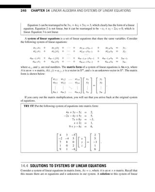
![14.4 SOLUTIONS TO SYSTEMS OF LINEAR EQUATIONS 247
equations is an x in Rn that satisfies the matrix form equation. Depending on the values that populate
A and y, there are three distinct possible solutions for x. Either there is no solution for x, or there is
one unique solution for x, or there are infinitely many solutions for x. This fact is not shown in this
text.
Case 1: There is no solution for x. If rank([A,y]) = rank(A) + 1 then y is linearly independent
from the columns of A. Therefore, because y is not in the range of A, by definition there cannot
be an x that satisfies the equation. Thus, comparing rank([A,y]) and rank(A) provides an easy
way to check if there are no solutions to a system of linear equations.
Case 2: There is a unique solution for x. If rank([A,y]) = rank(A), then y can be written as a
linear combination of the columns of A, and there is at least one solution for the matrix equation.
For there to be only one solution, rank(A) = n must also be true. In other words, the number of
equations must be exactly equal to the number of unknowns. To see why this property results in a
unique solution, consider the following three relationships between m and n : m n,m = n, and
m n.
• For the case m n, rank(A) = n cannot possibly be true because this means we have a “fat”
matrix with fewer equations than unknowns. Thus, we do not need to consider this subcase.
• When m = n and rank(A) = n, A is square and invertible. Since the inverse of a matrix is
unique, the matrix equation Ax = y can be solved by multiplying each side of the equation on
the left by A−1. This results in A−1Ax = A−1y → Ix = A−1y → x = A−1y, which gives the
unique solution to the equation.
• If m n, then there are more equations than unknowns; however, if rank(A) = n, then it is
possible to choose n equations (i.e., rows of A) such that if these equations are satisfied, then
the remaining m − n equations will also be satisfied. In other words, they are redundant. If the
m − n redundant equations are removed from the system, then the resulting system has an A
matrix that is n × n and invertible. These facts are not proven in this text. The new system then
has a unique solution, which is valid for the whole system.
Case 3: There are infinitely many solutions for x. If rank([A,y]) = rank(A), then y is in the
range of A, and there is at least one solution for the matrix equation; however, if rank(A) n,
then there are infinitely many solutions. Although it is not shown here, if rank(A) n, then there
is at least one nonzero vector, n, that is in the null space of A (Actually, there are infinitely
many null space vectors under these conditions.). If n is in the nullspace of A, then An = 0 by
definition. Now if x∗ is a solution to the matrix equation Ax = y, then, necessarily, Ax∗ = y;
however, Ax∗ + An = y or A(x∗ + n) = y. Therefore, x∗ + n is also a solution for Ax = y. In
fact, since A is a linear transformation, x∗ + αn is a solution for any real number α (you should
try to show this on your own). Since there are infinitely many acceptable values for α, there are
infinitely many solutions for the matrix equation.
The rest of the chapter will discuss how to solve a system of equations which has a unique solution.
First, we will discuss some of the common methods that you will most likely come across in your work
and then we will show you how to solve systems in Python.](https://image.slidesharecdn.com/pythonprogrammingandnumericalmethodsaguideforengineersand-231017183839-0fbc5295/85/Python_Programming_and_Numerical_Methods_A_Guide_for_Engineers_and-pdf-256-320.jpg)
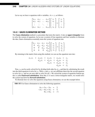
![14.4 SOLUTIONS TO SYSTEMS OF LINEAR EQUATIONS 249
Step 1: Turn these equations to the matrix form Ax = y.
⎡
⎣
4 3 −5
−2 −4 5
8 8 0
⎤
⎦
⎡
⎣
x1
x2
x3
⎤
⎦ =
⎡
⎣
2
5
−3
⎤
⎦.
Step 2: Obtain the augmented matrix [A,y] as
[A,y] =
⎡
⎣
4 3 −5 2
−2 −4 5 5
8 8 0 −3
⎤
⎦.
Step 3: Start eliminating the elements in the matrix by choosing a pivot equation, which is
used to eliminate the elements in other equations. Choose the first equation as the pivot equation
and turn the second row’s first element to zero by multiplying the first row (pivot equation) by
−0.5 and subtracting it from the second row. The multiplier is m2,1 = −0.5, giving us
⎡
⎣
4 3 −5 2
0 −2.5 2.5 6
8 8 0 −3
⎤
⎦.
Step 4: Turn the third row’s first element to zero. As was done above, we multiply the first row
by 2 and subtract it from the third row. The multiplier is m3,1 = 2, giving us
⎡
⎣
4 3 −5 2
0 −2.5 2.5 6
0 2 10 −7
⎤
⎦.
Step 5: Turn the third row’s second element to zero. We multiply the second row by −4/5 and
subtract it from the third row. The multiplier is m3,2 = −0.8, giving us
⎡
⎣
4 3 −5 2
0 −2.5 2.5 6
0 0 12 −2.2
⎤
⎦.
Step 6: We then obtain x3 = −2.2/12 = −0.183.
Step 7: If we insert x3 into the second equation, we obtain x2 = −2.583.
Step 8: If we insert x2 and x3 into the first equation, we obtain x1 = 2.208.
Note! Sometimes the first element in the first row is zero. When this is the case, switch the first row
with a nonzero first element row, then follow the same procedure as outlined above.
We are using the “pivoting” Gauss elimination method here. Note that there is also a “naive” Gauss
elimination method which assumes that the pivot values will never be zero.](https://image.slidesharecdn.com/pythonprogrammingandnumericalmethodsaguideforengineersand-231017183839-0fbc5295/85/Python_Programming_and_Numerical_Methods_A_Guide_for_Engineers_and-pdf-258-320.jpg)
![250 CHAPTER 14 LINEAR ALGEBRA AND SYSTEMS OF LINEAR EQUATIONS
14.4.2 GAUSS–JORDAN ELIMINATION METHOD
Gauss–Jordan elimination solves systems of equations. It is a procedure to turn A into a diagonal form
such that the matrix form of the equations becomes
⎡
⎢
⎢
⎣
1 0 0 0
0 1 0 0
0 0 1 0
0 0 0 1
⎤
⎥
⎥
⎦
⎡
⎢
⎢
⎣
x1
x2
x3
x4
⎤
⎥
⎥
⎦ =
⎡
⎢
⎢
⎢
⎣
y1
y2
y3
y4
⎤
⎥
⎥
⎥
⎦
.
Essentially, the equations become:
x1 + 0 + 0 + 0 = y1,
0 + x2 + 0 + 0 = y2,
0 + 0 + x3 + 0 = y3,
0 + 0 + 0 + x4 = y4.
Let us solve another equation system by using the above example as a blueprint.
TRY IT! Use Gauss–Jordan elimination to solve the following equations:
4x1 + 3x2 − 5x3 = 2,
−2x1 − 4x2 + 5x3 = 5,
8x1 + 8x2 = −3.
Step 1: Construct the augmented matrix [A,y],
[A,y] =
⎡
⎣
4 3 −5 2
−2 −4 5 5
8 8 0 −3
⎤
⎦.
Step 2: The first element in the first row should be 1, so we divide the row by 4:
⎡
⎣
1 3/4 −5/4 1/2
−2 −4 5 5
8 8 0 −3
⎤
⎦.
Step 3: To eliminate the first element in the second and third rows, we multiply the first row
by −2 and 8, respectively, and then subtract it from the second and third rows to get
⎡
⎣
1 3/4 −5/4 1/2
0 −5/2 5/2 6
0 2 10 −7
⎤
⎦.](https://image.slidesharecdn.com/pythonprogrammingandnumericalmethodsaguideforengineersand-231017183839-0fbc5295/85/Python_Programming_and_Numerical_Methods_A_Guide_for_Engineers_and-pdf-259-320.jpg)
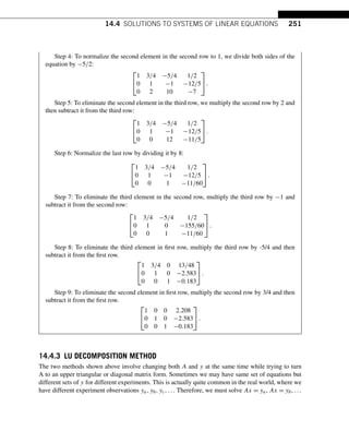
![252 CHAPTER 14 LINEAR ALGEBRA AND SYSTEMS OF LINEAR EQUATIONS
many times, since every time the [A,y] will change. Obviously, this is really inefficient. Is there a
method by which we only change the left side of A but not the right-hand side y?
The LU decomposition method changes the matrix A only, instead of y. It is ideal for solving the
system with the same coefficient matrices A but different constant vectors y. The LU decomposition
method aims to turn A into the product of two matrices L and U, where L is a lower triangular matrix
while U is an upper triangular matrix. With this decomposition, we convert the system of equations to
the following form:
LUx = y →
⎡
⎢
⎢
⎣
l1,1 0 0 0
l2,1 l2,2 0 0
l3,1 l3,2 l3,3 0
l4,1 l4,2 l4,3 l4,4
⎤
⎥
⎥
⎦
⎡
⎢
⎢
⎣
u1,1 u1,2 u1,3 u1,4
0 u2,2 u2,3 u2,4
0 0 u3,3 u3,4
0 0 0 u4,4
⎤
⎥
⎥
⎦
⎡
⎢
⎢
⎣
x1
x2
x3
x4
⎤
⎥
⎥
⎦ =
⎡
⎢
⎢
⎣
y1
y2
y3
y4
⎤
⎥
⎥
⎦.
If we define Ux = M, then the above equations become:
⎡
⎢
⎢
⎣
l1,1 0 0 0
l2,1 l2,2 0 0
l3,1 l3,2 l3,3 0
l4,1 l4,2 l4,3 l4,4
⎤
⎥
⎥
⎦M =
⎡
⎢
⎢
⎣
y1
y2
y3
y4
⎤
⎥
⎥
⎦.
We can easily solve the above problem by forward substitution (the opposite of the backward sub-
stitution as we saw in Gauss elimination method). After we solve for M, we can easily solve the rest
of the problem using backward substitution:
⎡
⎢
⎢
⎣
u1,1 u1,2 u1,3 u1,4
0 u2,2 u2,3 u2,4
0 0 u3,3 u3,4
0 0 0 u4,4
⎤
⎥
⎥
⎦
⎡
⎢
⎢
⎣
x1
x2
x3
x4
⎤
⎥
⎥
⎦ =
⎡
⎢
⎢
⎣
m1
m2
m3
m4
⎤
⎥
⎥
⎦.
But how do we obtain the L and U matrices? There are different ways to obtain the LU decompo-
sition. Below is one example that uses the Gauss elimination method. From the above, we know that
we obtain an upper triangular matrix after we conduct the Gauss elimination. At the same time, we
also obtain the lower triangular matrix even though it is never explicitly written out. During the Gauss
elimination procedure, the matrix A actually turns into the product of two matrices as shown below.
The right upper triangular matrix is the one we obtained earlier. The diagonal elements in the left lower
triangular matrix are 1, and the elements below the diagonal elements are the multipliers that multiply
the pivot equations to eliminate the elements during the calculation:
A =
⎡
⎢
⎢
⎣
1 0 0 0
m2,1 1 0 0
m3,1 m3,2 1 0
m4,1 m4,2 m4,3 1
⎤
⎥
⎥
⎦
⎡
⎢
⎢
⎣
u1,1 u1,2 u1,3 u1,4
0 u2,2 u2,3 u2,4
0 0 u3,3 u3,4
0 0 0 u4,4
⎤
⎥
⎥
⎦.
Note that we obtain both L and U at the same time when we perform the Gauss elimination. Using
the above example, where U is the one we used before to solve the equations, and L is composed of](https://image.slidesharecdn.com/pythonprogrammingandnumericalmethodsaguideforengineersand-231017183839-0fbc5295/85/Python_Programming_and_Numerical_Methods_A_Guide_for_Engineers_and-pdf-261-320.jpg)
![14.4 SOLUTIONS TO SYSTEMS OF LINEAR EQUATIONS 253
the multipliers (you can check the examples in the Gauss elimination section), we obtain:
L =
⎡
⎣
1 0 0
−0.5 1 0
2 −0.8 1
⎤
⎦,
U =
⎡
⎣
4 3 −5
0 −2.5 2.5
0 0 60
⎤
⎦.
TRY IT! Verify that the above L and U matrices are the LU decomposition of matrix A. The
result should be A = LU.
In [1]: import numpy as np
u = np.array([[4, 3, -5],
[0, -2.5, 2.5],
[0, 0, 12]])
l = np.array([[1, 0, 0],
[-0.5, 1, 0],
[2, -0.8, 1]])
print(LU=, np.dot(l, u))
LU= [[ 4. 3. -5.]
[-2. -4. 5.]
[ 8. 8. 0.]]
14.4.4 ITERATIVE METHODS – GAUSS–SEIDEL METHOD
The methods introduced above are all direct methods where the solution is computed using a finite
number of operations. This section introduces a different class of methods, namely the iterative meth-
ods, or indirect methods. They start with an initial guess of the solution and then repeatedly improve
the solution until the change of the solution is below a chosen threshold. In order to use this iterative
process, we first need to write the explicit form of a system of equations. If we have a system of linear
equations
⎡
⎢
⎢
⎢
⎣
a1,1 a1,2 ... a1,n
a2,1 a2,2 ... a2,n
.
.
.
.
.
.
...
.
.
.
am,1 am,2 ... am,n
⎤
⎥
⎥
⎥
⎦
⎡
⎢
⎢
⎢
⎣
x1
x2
.
.
.
xn
⎤
⎥
⎥
⎥
⎦
=
⎡
⎢
⎢
⎢
⎣
y1
y2
.
.
.
ym
⎤
⎥
⎥
⎥
⎦
,](https://image.slidesharecdn.com/pythonprogrammingandnumericalmethodsaguideforengineersand-231017183839-0fbc5295/85/Python_Programming_and_Numerical_Methods_A_Guide_for_Engineers_and-pdf-262-320.jpg)
![254 CHAPTER 14 LINEAR ALGEBRA AND SYSTEMS OF LINEAR EQUATIONS
we can write its explicit form as
xi =
1
ai,i
yi −
j=n
j=1,j=i
ai,j xj
.
This is the basics of the iterative methods; we can assume initial values for all the x, and use it as
x(0). In the first iteration, we can substitute x(0) into the right-hand side of the explicit equation above
to obtain the first iteration solution x(1). By substituting x(1) into the equation, we obtain x(2), and the
iterations continue until the difference between x(k) and x(k−1) is smaller than some predefined value.
Iterative methods require having specific conditions for the solution to converge. A sufficient, but
not necessary, condition of the convergence is that the coefficient matrix a is diagonally dominant.
This means that in each row of the matrix of coefficients a, the absolute value of the diagonal element
is greater than the sum of the absolute values of the off-diagonal elements. If the coefficient matrix
satisfies this condition, the iterations will converge to the solution. Note that the solution process might
still converge even when this condition is not satisfied.
14.4.4.1 Gauss–Seidel Method
The Gauss–Seidel method is a specific iterative method that is always using the latest estimated value
for each element in x. For example, first assume that the initial values for x2,x3,...,xn (except for
x1) are given and calculate x1. Using the calculated x1 and the rest of the x (except for x2), we can
calculate x2. Continuing in the same manner and calculating all the elements in x will conclude the
first iteration. The unique part of the Gauss–Seidel method is the use of the latest value to calculate the
next value in x. Such iterations are continued until the value converges. Let us use this method to solve
the same problem we just solved above.
EXAMPLE: Solve the following system of linear equations using Gauss–Seidel method using a
predefined threshold = 0.01. Remember to check if the converge condition is satisfied or not.
8x1 + 3x2 − 3x3 = 14,
−2x1 − 8x2 + 5x3 = 5,
3x1 + 5x2 + 10x3 = −8.
Let us first check if the coefficient matrix is diagonally dominant or not.
In [2]: a = [[8, 3, -3], [-2, -8, 5], [3, 5, 10]]
# Find diagonal coefficients
diag = np.diag(np.abs(a))
# Find row sum without diagonal
off_diag = np.sum(np.abs(a), axis=1) - diag
if np.all(diag off_diag):](https://image.slidesharecdn.com/pythonprogrammingandnumericalmethodsaguideforengineersand-231017183839-0fbc5295/85/Python_Programming_and_Numerical_Methods_A_Guide_for_Engineers_and-pdf-263-320.jpg)
![14.4 SOLUTIONS TO SYSTEMS OF LINEAR EQUATIONS 255
print(matrix is diagonally dominant)
else:
print(NOT diagonally dominant)
matrix is diagonally dominant
Since it is guaranteed to converge, we can use Gauss–Seidel method to solve the system.
In [3]: x1 = 0
x2 = 0
x3 = 0
epsilon = 0.01
converged = False
x_old = np.array([x1, x2, x3])
print(Iteration results)
print( k, x1, x2, x3 )
for k in range(1, 50):
x1 = (14-3*x2+3*x3)/8
x2 = (5+2*x1-5*x3)/(-8)
x3 = (-8-3*x1-5*x2)/(-5)
x = np.array([x1, x2, x3])
# check if it is smaller than threshold
dx = np.sqrt(np.dot(x-x_old, x-x_old))
print(%d, %.4f, %.4f, %.4f%(k, x1, x2, x3))
if dx epsilon:
converged = True
print(Converged!)
break
# assign the latest x value to the old value
x_old = x
if not converged:
print(Not converged, increase the # of iterations)
Iteration results
k, x1, x2, x3
1, 1.7500, -1.0625, 1.5875
2, 2.7437, -0.3188, 2.9275
3, 2.9673, 0.4629, 3.8433](https://image.slidesharecdn.com/pythonprogrammingandnumericalmethodsaguideforengineersand-231017183839-0fbc5295/85/Python_Programming_and_Numerical_Methods_A_Guide_for_Engineers_and-pdf-264-320.jpg)
![256 CHAPTER 14 LINEAR ALGEBRA AND SYSTEMS OF LINEAR EQUATIONS
4, 3.0177, 1.0226, 4.4332
5, 3.0290, 1.3885, 4.8059
6, 3.0315, 1.6208, 5.0397
7, 3.0321, 1.7668, 5.1861
8, 3.0322, 1.8582, 5.2776
9, 3.0322, 1.9154, 5.3348
10, 3.0323, 1.9512, 5.3705
11, 3.0323, 1.9735, 5.3929
12, 3.0323, 1.9875, 5.4068
13, 3.0323, 1.9962, 5.4156
14, 3.0323, 2.0017, 5.4210
Converged!
14.5 SOLVING SYSTEMS OF LINEAR EQUATIONS IN PYTHON
The examples presented above demonstrated the various methods you can use to solve systems of linear
equations. This is also very easy to do in Python, as shown below. The easiest way to get a solution is
via the solve function in NumPy.
TRY IT! Use numpy.linalg.solve to solve the following equations:
4x1 + 3x2 − 5x3 = 2,
−2x1 − 4x2 + 5x3 = 5,
8x1 + 8x2 = −3.
In [1]: import numpy as np
A = np.array([[4, 3, -5],
[-2, -4, 5],
[8, 8, 0]])
y = np.array([2, 5, -3])
x = np.linalg.solve(A, y)
print(x)
[ 2.20833333 -2.58333333 -0.18333333]
We get the same results as those in the previous section when calculated by hand. Under the “hood,”
the solver is actually doing an LU decomposition to get the results. If you can check the help of
the function, you will see it needs the input matrix to be square and of full rank, i.e., all rows (or,
equivalently, columns) must be linearly independent.](https://image.slidesharecdn.com/pythonprogrammingandnumericalmethodsaguideforengineersand-231017183839-0fbc5295/85/Python_Programming_and_Numerical_Methods_A_Guide_for_Engineers_and-pdf-265-320.jpg)
![14.5 SOLVING SYSTEMS OF LINEAR EQUATIONS IN PYTHON 257
TRY IT! Try to solve the above equations using the matrix inversion approach.
In [2]: A_inv = np.linalg.inv(A)
x = np.dot(A_inv, y)
print(x)
[ 2.20833333 -2.58333333 -0.18333333]
We can also obtain the L and U matrices used in the LU decomposition using the SciPy
package.
TRY IT! Get the L and U for the above matrix A.
In [3]: from scipy.linalg import lu
P, L, U = lu(A)
print(P:n, P)
print(L:n, L)
print(U:n, U)
print(LU:n,np.dot(L, U))
P:
[[0. 0. 1.]
[0. 1. 0.]
[1. 0. 0.]]
L:
[[ 1. 0. 0. ]
[-0.25 1. 0. ]
[ 0.5 0.5 1. ]]
U:
[[ 8. 8. 0. ]
[ 0. -2. 5. ]
[ 0. 0. -7.5]]
LU:
[[ 8. 8. 0.]
[-2. -4. 5.]
[ 4. 3. -5.]]
Why do we obtain different L and U from those calculated by hand in the last section? You will
also see that there is a permutation matrix P that is returned by the lu function. This permutation
matrix records how it changes the order of the equations for easier calculation purposes. For example,](https://image.slidesharecdn.com/pythonprogrammingandnumericalmethodsaguideforengineersand-231017183839-0fbc5295/85/Python_Programming_and_Numerical_Methods_A_Guide_for_Engineers_and-pdf-266-320.jpg)
![258 CHAPTER 14 LINEAR ALGEBRA AND SYSTEMS OF LINEAR EQUATIONS
if the first element in the first row is zero, it cannot be the pivot equation since you cannot turn the first
elements in other rows to zero; therefore, we need to switch the order of the equations to get a new
pivot equation. If you multiply P and A, you will see that this permutation matrix reverses the order of
the equations for this case.
TRY IT! Multiply P and A and see what is the effect of the permutation matrix on A.
In [4]: print(np.dot(P, A))
[[ 8. 8. 0.]
[-2. -4. 5.]
[ 4. 3. -5.]]
14.6 MATRIX INVERSION
We defined the inverse of a square matrix M as a matrix of the same size, M−1, such that M · M−1 =
M−1 · M = I. If the dimension of the matrix is high, the analytical solution for the matrix inversion
will be complicated. Therefore, we need some other efficient ways to obtain the inverse of the matrix.
Let us use a 4 × 4 matrix for illustration. Suppose we have
M =
⎡
⎢
⎢
⎣
m1,1 m1,2 m1,3 m1,4
m2,1 m2,2 m2,3 m2,4
m3,1 m3,2 m3,3 m3,4
m4,1 m4,2 m4,3 m4,4
⎤
⎥
⎥
⎦,
and the inverse of M is
X =
⎡
⎢
⎢
⎣
x1,1 x1,2 x1,3 x1,4
x2,1 x2,2 x2,3 x2,4
x3,1 x3,2 x3,3 x3,4
x4,1 x4,2 x4,3 x4,4
⎤
⎥
⎥
⎦.
Therefore, we will have:
M · X =
⎡
⎢
⎢
⎣
m1,1 m1,2 m1,3 m1,4
m2,1 m2,2 m2,3 m2,4
m3,1 m3,2 m3,3 m3,4
m4,1 m4,2 m4,3 m4,4
⎤
⎥
⎥
⎦
⎡
⎢
⎢
⎣
x1,1 x1,2 x1,3 x1,4
x2,1 x2,2 x2,3 x2,4
x3,1 x3,2 x3,3 x3,4
x4,1 x4,2 x4,3 x4,4
⎤
⎥
⎥
⎦ =
⎡
⎢
⎢
⎣
1 0 0 0
0 1 0 0
0 0 1 0
0 0 0 1
⎤
⎥
⎥
⎦.
We can rewrite the above equation as four separate equations, i.e.,
⎡
⎢
⎢
⎣
m1,1 m1,2 m1,3 m1,4
m2,1 m2,2 m2,3 m2,4
m3,1 m3,2 m3,3 m3,4
m4,1 m4,2 m4,3 m4,4
⎤
⎥
⎥
⎦
⎡
⎢
⎢
⎣
x1,1
x2,1
x3,1
x4,1
⎤
⎥
⎥
⎦ =
⎡
⎢
⎢
⎣
1
0
0
0
⎤
⎥
⎥
⎦,](https://image.slidesharecdn.com/pythonprogrammingandnumericalmethodsaguideforengineersand-231017183839-0fbc5295/85/Python_Programming_and_Numerical_Methods_A_Guide_for_Engineers_and-pdf-267-320.jpg)
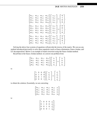
![260 CHAPTER 14 LINEAR ALGEBRA AND SYSTEMS OF LINEAR EQUATIONS
In summary, all we need to do is to convert
⎡
⎢
⎢
⎣
m1,1 m1,2 m1,3 m1,4 1 0 0 0
m2,1 m2,2 m2,3 m2,4 0 1 0 0
m3,1 m3,2 m3,3 m3,4 0 0 1 0
m4,1 m4,2 m4,3 m4,4 0 0 0 1
⎤
⎥
⎥
⎦
to
⎡
⎢
⎢
⎢
⎣
1 0 0 0 m1,1 m1,2 m1,3 m1,4
0 1 0 0 m2,1 m2,2 m2,3 m2,4
0 0 1 0 m3,1 m3,2 m3,3 m1,4
0 0 0 1 m4,1 m4,2 m4,3 m1,4
⎤
⎥
⎥
⎥
⎦
.
Then the matrix
⎡
⎢
⎢
⎢
⎣
m1,1 m1,2 m1,3 m1,4
m2,1 m2,2 m2,3 m2,4
m3,1 m3,2 m3,3 m1,4
m4,1 m4,2 m4,3 m1,4
⎤
⎥
⎥
⎥
⎦
is the inverse of M we are looking for.
Can you explain how to use LU decomposition to get the inverse of a matrix?
14.7 SUMMARY AND PROBLEMS
14.7.1 SUMMARY
1. Linear algebra is the foundation of many engineering fields.
2. Vectors can be considered as points in Rn; addition and multiplication are defined, although this is
not necessarily the case for scalars.
3. A set of vectors is linearly independent if none of the vectors can be written as a linear combination
of the others.
4. Matrices are tables of numbers. They have several important characteristics including the determi-
nant, rank, and inverse.
5. A system of linear equations can be represented by the matrix equation Ax = y.
6. The number of solutions to a system of linear equations is related to rank(A) and rank([A,y]). It
can be zero, one, or infinity.
7. We can solve the equations using Gauss elimination, Gauss–Jordan elimination, LU decomposition,
and the Gauss–Seidel method.
8. We introduced methods to find the matrix inverse.](https://image.slidesharecdn.com/pythonprogrammingandnumericalmethodsaguideforengineersand-231017183839-0fbc5295/85/Python_Programming_and_Numerical_Methods_A_Guide_for_Engineers_and-pdf-269-320.jpg)
![14.7 SUMMARY AND PROBLEMS 261
14.7.2 PROBLEMS
1. It is strongly recommended that you read a book on linear algebra, which will give you greater
mastery of the contents of this chapter. We strongly recommend reading the first part of book
Optimization Models by Giuseppe Calafiore and Laurent El Ghaoui to get you started.
2. Show that matrix multiplication distributes over matrix addition: show A(B + C) = AB + AC
assuming that A,B, and C are matrices of compatible size.
3. Write a function my_is_orthogonal(v1,v2,tol) where v1 and v2 are column vectors of the same
size, and tol is a scalar value strictly larger than zero. The output should be 1 if the angle between
v1 and v2 is within tol of π/2, that is, |π/2 − θ| tol, and zero otherwise. You may assume that
v1 and v2 are column vectors of the same size, and that tol is a positive scalar.
In [ ]: # Test cases for Problem 3
a = np.array([[1], [0.001]])
b = np.array([[0.001], [1]])
# output: 1
my_is_orthogonal(a,b, 0.01)
# output: 0
my_is_orthogonal(a,b, 0.001)
# output: 0
a = np.array([[1], [0.001]])
b = np.array([[1], [1]])
my_is_orthogonal(a,b, 0.01)
# output: 1
a = np.array([[1], [1]])
b = np.array([[-1], [1]])
my_is_orthogonal(a,b, 1e-10)
3. Write a function my_is_similar(s1,s2,tol) where s1 and s2 are strings, not necessarily of the
same size, and tol is a scalar value strictly larger than zero. From s1 and s2, the function should
construct two vectors, v1 and v2, where v1[0] is the number of a’s in s1, v1[1] is the number b’s
in s1, and so on until v1[25], which is the number of z’s in v1. The vector v2 should be similarly
constructed from s2. The output should be 1 if the absolute value of the angle between v1 and v2
is less than tol, that is, |θ| tol.
4. Write a function my_make_lin_ind(A) where A and B are matrices. Let rank(A) = n. Then B
should be a matrix containing the first n columns of A that are all linearly independent. Note that
this implies that B has full rank.
In [ ]: ## Test cases for Problem 4
A = np.array([[12,24,0,11,-24,18,15],
[19,38,0,10,-31,25,9],](https://image.slidesharecdn.com/pythonprogrammingandnumericalmethodsaguideforengineersand-231017183839-0fbc5295/85/Python_Programming_and_Numerical_Methods_A_Guide_for_Engineers_and-pdf-270-320.jpg)
![262 CHAPTER 14 LINEAR ALGEBRA AND SYSTEMS OF LINEAR EQUATIONS
[1,2,0,21,-5,3,20],
[6,12,0,13,-10,8,5],
[22,44,0,2,-12,17,23]])
B = my_make_lin_ind(A)
# B = [[12,11,-24,15],
# [19,10,-31,9],
# [1,21,-5,20],
# [6,13,-10,5],
# [22,2,-12,23]]
5. Cramer’s rule is a method of computing the determinant of a matrix. Consider an n × n square
matrix M. Let M(i,j) be the element of M in the ith row and jth column of M, and let mi,j be
the minor of M created by removing the ith row and jth column from M. Cramer’s rule says that
det(M) =
n
i=1
(−1)i−1
M(1,i)det(mi,j ).
Write a function my_rec_det(M) where the output is det(M). Use Cramer’s rule to compute the
determinant, not NumPy’s function.
6. What is the complexity of my_rec_det in the previous problem? Do you think this is an effective
way of determining if a matrix is singular or not?
7. Let p be a vector with length L containing the coefficients of a polynomial of order L − 1. For
example, the vector p = [1,0,2] is a representation of the polynomial f (x) = 1x2 + 0x + 2. Write
a function my_poly_der_mat(p) where p is the aforementioned vector, and the output D is the
matrix that will return the coefficients of the derivative of p when p is left multiplied by D. For
example, the derivative of f (x) is f (x) = 2x; therefore, d = Dp should yield d = [2,0]. Note
this implies that the dimension of D is L − 1 × L. The point of this problem is to show that
differentiating polynomials is actually a linear transformation.
8. Use the Gauss elimination method to solve the following equations:
3x1 − x2 + 4x3 = 2,
17x1 + 2x2 + x3 = 14,
x1 + 12x2 − 7z = 54.
9. Use the Gauss–Jordan elimination method to solve the equations in Problem 8.
10. Obtain the lower triangular matrix L and upper triangular matrix U from the equations in Prob-
lem 8.
11. Show that the dot-product distributes across vector addition, that is, show that u · (v + w) = u ·
v + u · w.](https://image.slidesharecdn.com/pythonprogrammingandnumericalmethodsaguideforengineersand-231017183839-0fbc5295/85/Python_Programming_and_Numerical_Methods_A_Guide_for_Engineers_and-pdf-271-320.jpg)
![14.7 SUMMARY AND PROBLEMS 263
FIGURE 14.1
Graph for Problem 12.
12. Consider the following network shown in Fig. 14.1 consisting of two power supply stations de-
noted by S1 and S2 and five power recipient nodes denoted by N1 to N5. The nodes are connected
by power lines, which are denoted by arrows, and power can flow between nodes along these lines
in both directions.
Let di be a positive scalar denoting the power demand for node i; assume that this demand must be
met exactly. The capacity of the power supply stations is denoted by S. Power supply stations must
run at capacity. For each arrow, let fj be the power flow along that arrow. Negative flow implies
that power is running in the opposite direction of the arrow.
Write a function my_flow_calculator(S,d) where S is a 1 × 2 vector representing the capacity
of each power supply station, and d is a 1 × 5 row vector representing the demands at each node
(i.e., d[0] is the demand at node 1). The output argument, f, should be a 1 × 7 row vector denoting
the flows in the network (i.e., f[0] = f1 in the diagram). The flows contained in f should satisfy
all the constraints of the system, like power generation and demands. Note that there may be more
than one solution to the system of equations.
The total flow into a node must equal the total flow out of the node plus the demand; that is, for
each node i,finflow = foutflow + di. You may assume that
Sj =
di.
In [ ]: ## Test cases for Problem 12
s = np.array([[10, 10]])
d = np.array([[4, 4, 4, 4, 4]])
# f = [[10.0, 4.0, -2.0, 4.5, 5.5, 2.5, 1.5]]
f = my_flow_calculator(s, d)
s = np.array([[10, 10]])
d = np.array([[3, 4, 5, 4, 4]])
# f = [[10.0, 5.0, -1.0, 4.5, 5.5, 2.5, 1.5]]
f = my_flow_calculator(s, d)](https://image.slidesharecdn.com/pythonprogrammingandnumericalmethodsaguideforengineersand-231017183839-0fbc5295/85/Python_Programming_and_Numerical_Methods_A_Guide_for_Engineers_and-pdf-272-320.jpg)
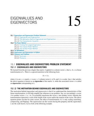
![266 CHAPTER 15 EIGENVALUES AND EIGENVECTORS
TRY IT! Plot the vector x = [[1], [1]] and the vector b = Ax, where A = [[2, 0], [0, 1]]
In [1]: import numpy as np
import matplotlib.pyplot as plt
plt.style.use(seaborn-poster)
%matplotlib inline
def plot_vect(x, b, xlim, ylim):
function to plot two vectors,
x - the original vector
b - the transformed vector
xlim - the limit for x
ylim - the limit for y
plt.figure(figsize = (10, 6))
plt.quiver(0,0,x[0],x[1],
color=k,angles=xy,
scale_units=xy,scale=1,
label=Original vector)
plt.quiver(0,0,b[0],b[1],
color=g,angles=xy,
scale_units=xy,scale=1,
label =Transformed vector)
plt.xlim(xlim)
plt.ylim(ylim)
plt.xlabel(X)
plt.ylabel(Y)
plt.legend()
plt.show()
In [2]: A = np.array([[2, 0],[0, 1]])
x = np.array([[1],[1]])
b = np.dot(A, x)
plot_vect(x,b,(0,3),(0,2))](https://image.slidesharecdn.com/pythonprogrammingandnumericalmethodsaguideforengineersand-231017183839-0fbc5295/85/Python_Programming_and_Numerical_Methods_A_Guide_for_Engineers_and-pdf-274-320.jpg)
![15.1 EIGENVALUES AND EIGENVECTORS PROBLEM STATEMENT 267
We can see from the generated figure that the original vector x is rotated and stretched longer after
being transformed by A. The vector [[1], [1]] is transformed to [[2], [1]]. Let us try to do the same
exercise with a different vector [[1], [0]].
TRY IT! Plot the vector x = [[1], [0]] and the vector b = Ax where A = [[2, 0], [0, 1]]
In [3]: x = np.array([[1], [0]])
b = np.dot(A, x)
plot_vect(x,b,(0,3),(-0.5,0.5))
With this new vector, the only change after the transformation is the length of the vector; it is
stretched. The new vector is [[2], [0]], therefore, the transform is
Ax = 2x](https://image.slidesharecdn.com/pythonprogrammingandnumericalmethodsaguideforengineersand-231017183839-0fbc5295/85/Python_Programming_and_Numerical_Methods_A_Guide_for_Engineers_and-pdf-275-320.jpg)
![268 CHAPTER 15 EIGENVALUES AND EIGENVECTORS
with x = [[1], [0]] and λ = 2. The direction of the vector does not change at all (no rotation). You can
also check that [[0], [1]] is another eigenvector; try to verify this by yourself.
15.1.3 THE CHARACTERISTIC EQUATION
In order to get the eigenvalues and eigenvectors, from Ax = λx, we can use the following form:
(A − λI)x = 0,
where I is the identify matrix with the same dimensions as A. If matrix A − λI has an inverse and both
sides are multiplied by (A − λI)−1, we get a trivial solution x = 0. Therefore, the only interesting case
is when A − λI is singular (no inverse exists), and we have a nontrivial solution, which means that the
determinant is zero:
det(A − λI) = 0.
This equation is called the characteristic equation that will lead to a polynomial equation for λ,
which we can solve for the eigenvalues; see the example below.
TRY IT! Obtain the eigenvalues for matrix [[0, 2], [2, 3]]
The characteristic equation gives us
0 − λ 2
2 3 − λ
= 0.
Therefore, we have
−λ(3 − λ) − 4 = 0 ⇒ λ2
− 3λ − 4 = 0.
We obtain two eigenvalues:
λ1 = 4, λ2 = −1.
TRY IT! Obtain the eigenvectors for the above two eigenvalues.
If the first eigenvalue is λ1 = 4, we can simply insert it back to A − λI = 0, where we have:
−4 2
2 −1
x1
x2
=
0
0
.
Therefore, we have two equations −4x1 + 2x2 = 0 and 2x1 − x2 = 0, both indicating that x2 =
2x1. Therefore, the first eigenvector is
x1 = k1
1
2
.](https://image.slidesharecdn.com/pythonprogrammingandnumericalmethodsaguideforengineersand-231017183839-0fbc5295/85/Python_Programming_and_Numerical_Methods_A_Guide_for_Engineers_and-pdf-276-320.jpg)
![15.2 THE POWER METHOD 269
The symbol k1 is a scalar (k1 = 0); as long as we have the ratio between x2 and x1 as 2, it will
be an eigenvector. We can verify that the vector [[1], [2]] is an eigenvector by inserting it back:
0 2
2 3
1
2
=
4
8
= 4
1
2
.
By inserting λ2 = −1 as above, we obtain the other eigenvector as follows where k2 = 0:
x2 = k2
−2
1
.
The above example demonstrates how we can obtain the eigenvalues and eigenvectors from a matrix
A; the choice of the eigenvectors for a system is not unique. When you have a larger matrix A and try
to solve the nth order polynomial characteristic equation, the solution becomes more complicated.
Luckily, many different numerical methods have been developed to solve the eigenvalue problems for
larger matrices (with a few hundred to thousands of dimensions). We will introduce the power method
and the QR method in the next two sections.
15.2 THE POWER METHOD
15.2.1 FINDING THE LARGEST EIGENVALUE
Some problems only require finding the largest dominant eigenvalue and its corresponding eigenvector.
In this case, we can use the power method, which is an iterative method that will converge to the largest
eigenvalue; see the example below.
Consider an n × n matrix A that has n real eigenvalues λ1,λ2,...,λn and the corresponding lin-
early independent eigenvectors v1,v2,...,vn. Since the eigenvalues are scalars, we can rank them so
that
|λ1| |λ2| ≥ ··· ≥ |λn|.
Note that we only require |λ1| |λ2|; the other eigenvalues may be equal to each other.
Because the eigenvectors are assumed linearly independent, they are a set of basis vectors, which
means that any vector that is in the same space can be written as a linear combination of the basis
vectors. That is, for any vector x0 and can be written as:
x0 = c1v1 + c2v2 + ··· + cnvn
where c1 = 0 is the constraint. If it is zero, then we need to choose another initial vector so that c1 = 0.
Now let us multiply both sides by A:
Ax0 = c1Av1 + c2Av2 + ··· + cnAvn.
Since Avi = λivi,
Ax0 = c1λ1v1 + c2λ2v2 + ··· + cnλnvn.](https://image.slidesharecdn.com/pythonprogrammingandnumericalmethodsaguideforengineersand-231017183839-0fbc5295/85/Python_Programming_and_Numerical_Methods_A_Guide_for_Engineers_and-pdf-277-320.jpg)
![270 CHAPTER 15 EIGENVALUES AND EIGENVECTORS
We can change the above equation to:
Ax0 = c1λ1
v1 +
c2
c1
λ2
λ1
v2 + ··· +
cn
c1
λn
λ1
vn
= c1λ1x1,
where x1 is a new vector, x1 = v1 + c2
c1
λ2
λ1
v2 + ··· + cn
c1
λn
λ1
vn.
This finishes the first iteration. For the second iteration, we apply A to x1:
Ax1 = λ1v1 +
c2
c1
λ2
2
λ1
v2 + ··· +
cn
c1
λ2
n
λ1
vn.
Similarly, we can rearrange the above equation to get
Ax1 = λ1
v1 +
c2
c1
λ2
2
λ2
1
v2 + ··· +
cn
c1
λ2
n
λ2
1
vn
= λ1x2,
where x2 is a new vector, x2 = v1 + c2
c1
λ2
2
λ2
1
v2 + ··· + cn
c1
λ2
n
λ2
1
vn.
If we continue applying A to the new vector, we obtain from each iteration k:
Axk−1 = λ1
v1 +
c2
c1
λk
2
λk
1
v2 + ··· +
cn
c1
λk
n
λk
1
vn
= λ1xk.
Because λ1 is the largest eigenvalue, the ratio λi
λ1
1 for all i 1. When k is sufficiently large,
the factor (λn
λ1
)k will be close to zero, so that all terms that contain this factor can be neglected as k
increases:
Axk−1 ∼ λ1v1.
Essentially, if k is large enough, we will obtain the largest eigenvalue and its corresponding eigen-
vector. When implementing this power method, the resulting vector in each iteration is usually nor-
malized. This can be done by factoring out the largest element in the vector, which will make the
largest element in the vector equal to 1. This normalization will provide the largest eigenvalue and its
corresponding eigenvector at the same time; see the example below.
When should we stop the iteration? The basic stopping criterion should be one of these the follow-
ing: (1) the difference between eigenvalues is less than some specified tolerance; (2) the angle between
eigenvectors is smaller than a threshold; or (3) the norm of the residual vector is small enough.
TRY IT! We know from the last section that the largest eigenvalue is 4 for the matrix A =
0 2
2 3
.
Use the power method to find the largest eigenvalue and the associated eigenvector. You can use
the initial vector [1, 1] to start the iteration.](https://image.slidesharecdn.com/pythonprogrammingandnumericalmethodsaguideforengineersand-231017183839-0fbc5295/85/Python_Programming_and_Numerical_Methods_A_Guide_for_Engineers_and-pdf-278-320.jpg)
![15.2 THE POWER METHOD 271
First iteration:
0 2
2 3
1
1
=
2
5
= 5
0.4
1
.
Second iteration:
0 2
2 3
0.4
1
=
2
3.8
= 3.8
0.5263
1
.
Third iteration:
0 2
2 3
0.5263
1
=
2
4.0526
= 4.0526
0.4935
1
.
Fourth iteration:
0 2
2 3
0.4935
1
=
2
3.987
= 3.987
0.5016
1
.
Fifth iteration:
0 2
2 3
0.5016
1
=
2
4.0032
= 4.0032
0.4996
1
.
Sixth iteration:
0 2
2 3
0.4996
1
=
2
3.9992
= 3.9992
0.5001
1
.
Seventh iteration:
0 2
2 3
0.5001
1
=
2
4.0002
= 4.0002
0.5000
1
.
After seven iterations, the eigenvalue has converged to four, with [0.5, 1] as the corresponding
eigenvector.
TRY IT! Implement the power method in Python.
In [1]: import numpy as np
In [2]: def normalize(x):
fac = abs(x).max()
x_n = x / x.max()
return fac, x_n](https://image.slidesharecdn.com/pythonprogrammingandnumericalmethodsaguideforengineersand-231017183839-0fbc5295/85/Python_Programming_and_Numerical_Methods_A_Guide_for_Engineers_and-pdf-279-320.jpg)
![272 CHAPTER 15 EIGENVALUES AND EIGENVECTORS
In [3]: x = np.array([1, 1])
a = np.array([[0, 2],
[2, 3]])
for i in range(8):
x = np.dot(a, x)
lambda_1, x = normalize(x)
print(Eigenvalue:, lambda_1)
print(Eigenvector:, x)
Eigenvalue: 3.999949137887188
Eigenvector: [0.50000636 1.]
15.2.2 THE INVERSE POWER METHOD
The eigenvalues of the inverse matrix A−1 are the reciprocals of the eigenvalues of A. By taking
advantage of this feature, as well as the power method, we are able to obtain the smallest eigenvalue of
A; this will be basis of the inverse power method. The steps are very simple: instead of applying A as
described above, we just apply A−1 for our iteration to find the largest value of 1
λ1
, which will be the
smallest value of the eigenvalues for A. In practice, we can use the methods we covered in the previous
chapter to calculate the inverse of the matrix. We will not go to greater detail here, but we present an
example below.
TRY IT! Find the smallest eigenvalue and eigenvector for A =
0 2
2 3
.
In [4]: from numpy.linalg import inv
In [5]: a_inv = inv(a)
for i in range(8):
x = np.dot(a_inv, x)
lambda_1, x = normalize(x)
print(Eigenvalue:, lambda_1)
print(Eigenvector:, x)
Eigenvalue: 0.20000000000003912
Eigenvector: [1. 1.]](https://image.slidesharecdn.com/pythonprogrammingandnumericalmethodsaguideforengineersand-231017183839-0fbc5295/85/Python_Programming_and_Numerical_Methods_A_Guide_for_Engineers_and-pdf-280-320.jpg)
![15.3 THE QR METHOD 273
15.2.3 THE SHIFTED POWER METHOD
In some cases, it is necessary to find all the eigenvalues and eigenvectors instead of just the largest and
smallest. One simple, but inefficient way is to use the shifted power method; we will introduce you a
more efficient method in the next section.
Given Ax = λ1x, and λ1 being the largest eigenvalue obtained by the power method, we have
[A − λ1I]x = αx,
where α’s are the eigenvalues of the shifted matrix A − λ1I, which will be 0,λ2 − λ1,λ3 −
λ1,...,λn − λ1.
Now if we apply the power method to the shifted matrix, we can determine the largest eigenvalue of
the shifted matrix, i.e., αk. Since αk = λk − λ1, we can obtain the eigenvalue λk easily. Repeating this
process many times will find the all the other eigenvalues, but you can see it is very labor intensive. A
better method for finding all the eigenvalues is to use the QR method, which we will introduced next.
15.3 THE QR METHOD
The QR method is the preferred iterative method to find all the eigenvalues of a matrix (but not the
eigenvectors at the same time). The idea is based on the following two concepts:
1. Similar matrices will have the same eigenvalues and associated eigenvectors. Two square ma-
trices A and B are similar if
A = C−1
BC
where C is an invertible matrix.
2. The QR method is a way to decompose a matrix into two matrices Q and R, where Q is
an orthogonal matrix, and R is an upper triangular matrix. An orthogonal matrix satisfies
Q−1 = QT , which means Q−1Q = QT Q = I.
How do we link these two concepts to find the eigenvalues? Say, we have a matrix A0 whose eigen-
values must be determined. At the kth step (starting with k = 0), we can perform the QR decomposition
and obtain
Ak = QkRk
where Qk is an orthogonal matrix, and Rk is an upper triangular matrix. We then form
Ak+1 = RkQk
to obtain
Ak+1 = RkQk = Q−1
k QkRkQk = Q−1
k AkQk.
Because all the Ak are similar, as we discussed above, they all have the same eigenvalues.](https://image.slidesharecdn.com/pythonprogrammingandnumericalmethodsaguideforengineersand-231017183839-0fbc5295/85/Python_Programming_and_Numerical_Methods_A_Guide_for_Engineers_and-pdf-281-320.jpg)
![274 CHAPTER 15 EIGENVALUES AND EIGENVECTORS
As the iteration continues, we will eventually converge to an upper triangular matrix with the form:
Ak = RkQk =
⎡
⎢
⎢
⎢
⎣
λ1 X ... X
0 λ2 ... X
.
.
.
.
.
.
...
.
.
.
0 0 ... λn
⎤
⎥
⎥
⎥
⎦
,
where the diagonal values are the eigenvalues of the matrix. In each iteration of the QR method, fac-
toring a matrix into an orthogonal and an upper triangular matrix can be done by using a special matrix
called Householder matrix. We will not go into the mathematical details how you get the Q and R
from the matrix. Instead, we will use the Python function to obtain the two matrices directly.
TRY IT! Use the qr function in numpy.linalg to decompose matrix A =
0 2
2 3
. Verify the
results.
In [1]: import numpy as np
from numpy.linalg import qr
In [2]: a = np.array([[0, 2],
[2, 3]])
q, r = qr(a)
print(Q:, q)
print(R:, r)
b = np.dot(q, r)
print(QR:, b)
Q: [[ 0. -1.]
[-1. 0.]]
R: [[-2. -3.]
[ 0. -2.]]
QR: [[0. 2.]
[2. 3.]]
TRY IT! Use the QR method to get the eigenvalues of matrix A =
0 2
2 3
. Do 20 iterations, and
print out the first, fifth, 10th, and 20th iteration.](https://image.slidesharecdn.com/pythonprogrammingandnumericalmethodsaguideforengineersand-231017183839-0fbc5295/85/Python_Programming_and_Numerical_Methods_A_Guide_for_Engineers_and-pdf-282-320.jpg)
![15.4 EIGENVALUES AND EIGENVECTORS IN PYTHON 275
In [3]: a = np.array([[0, 2],
[2, 3]])
p = [1, 5, 10, 20]
for i in range(20):
q, r = qr(a)
a = np.dot(r, q)
if i+1 in p:
print(fIteration {i+1}:)
print(a)
Iteration 1:
[[3. 2.]
[2. 0.]]
Iteration 5:
[[ 3.99998093 0.00976559]
[ 0.00976559 -0.99998093]]
Iteration 10:
[[ 4.00000000e+00 9.53674316e-06]
[ 9.53674316e-06 -1.00000000e+00]]
Iteration 20:
[[ 4.00000000e+00 9.09484250e-12]
[ 9.09494702e-12 -1.00000000e+00]]
Note that after the fifth iteration, the eigenvalues are converged to the correct ones. The next section
will demonstrate how to obtain the eigenvalues and eigenvectors in Python using the built-in function.
15.4 EIGENVALUES AND EIGENVECTORS IN PYTHON
The methods introduced above are fairly complicated to execute. The calculation of eigenvalues and
eigenvectors in Python is fairly easy. The main built-in function in Python to solve the eigenval-
ue/eigenvector problem for a square array is the eig function in numpy.linalg; see below for an
example in how to execute it.
TRY IT! Calculate the eigenvalues and eigenvectors for matrix A =
0 2
2 3
.
In [1]: import numpy as np
from numpy.linalg import eig
In [2]: a = np.array([[0, 2],
[2, 3]])](https://image.slidesharecdn.com/pythonprogrammingandnumericalmethodsaguideforengineersand-231017183839-0fbc5295/85/Python_Programming_and_Numerical_Methods_A_Guide_for_Engineers_and-pdf-283-320.jpg)
![276 CHAPTER 15 EIGENVALUES AND EIGENVECTORS
w,v=eig(a)
print(E-value:, w)
print(E-vector, v)
E-value: [-1. 4.]
E-vector [[-0.89442719 -0.4472136 ]
[ 0.4472136 -0.89442719]]
TRY IT! Compute the eigenvalues and eigenvectors for the matrix A =
⎡
⎣
2 2 4
1 3 5
2 3 4
⎤
⎦.
In [3]: a = np.array([[2, 2, 4],
[1, 3, 5],
[2, 3, 4]])
w,v=eig(a)
print(E-value:, w)
print(E-vector, v)
E-value: [ 8.80916362 0.92620912 -0.73537273]
E-vector [[-0.52799324 -0.77557092 -0.36272811]
[-0.604391 0.62277013 -0.7103262 ]
[-0.59660259 -0.10318482 0.60321224]]
15.5 SUMMARY AND PROBLEMS
15.5.1 SUMMARY
1. Eigenvalues and eigenvectors help us understand the characteristics of a linear transformation.
2. Eigenvectors of a matrix are the vectors that can only be scaled lengthwise without rotation after
applying the matrix transformation; the eigenvalues are the factors of the scaling.
3. We can use power method to get the largest eigenvalue and corresponding eigenvector of a matrix.
4. The inverse power method can help us get the smallest eigenvalue and corresponding eigenvector
of a matrix.
5. The shifted power method can get all the other eigenvectors/eigenvectors of a matrix.
6. The preferred method to get all the eigenvalues is the QR method.
15.5.2 PROBLEMS
1. Write down the characteristic equation for matrix A =
3 2
5 3
.
2. Use the above characteristic equation to solve for eigenvalues and eigenvectors of matrix A.](https://image.slidesharecdn.com/pythonprogrammingandnumericalmethodsaguideforengineersand-231017183839-0fbc5295/85/Python_Programming_and_Numerical_Methods_A_Guide_for_Engineers_and-pdf-284-320.jpg)
![15.5 SUMMARY AND PROBLEMS 277
3. Use the first eigenvector derived from Problem 2 to verify that Ax = λx.
4. Use the power method to obtain the largest eigenvalue and eigenvector for the matrix A =
⎡
⎣
2 1 2
1 3 2
2 4 1
⎤
⎦. Start with initial vector [1, 1, 1] and see the results after eight iterations.
5. Using the inverse power method to get the smallest eigenvalue and eigenvector for the matrix in
Problem 4, see how many iterations are needed for it to converge to the smallest eigenvalue.
6. Perform a QR decomposition for matrix A in Problem 4. Verify that A = QR and Q is an orthogonal
matrix.
7. Use the QR method to get all the eigenvalues for matrix A in Problem 4.
8. Obtain the eigenvalues and eigenvectors for matrix A in Problem 4 using the Python built-in func-
tion.](https://image.slidesharecdn.com/pythonprogrammingandnumericalmethodsaguideforengineersand-231017183839-0fbc5295/85/Python_Programming_and_Numerical_Methods_A_Guide_for_Engineers_and-pdf-285-320.jpg)
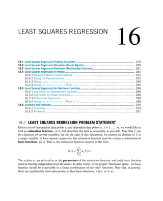
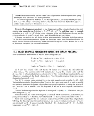

![282 CHAPTER 16 LEAST SQUARES REGRESSION
With some rearrangement, the previous expression can be manipulated as follows:
m
i=1
n
j=1
αj fj (xi)fk(xi) −
m
i=1
yifk(xi) = 0,
and upon further rearrangement (we take advantage of the fact that addition commutes) the result is
n
j=1
αj
m
i=1
fj (xi)fk(xi) =
m
i=1
yifk(xi).
Now let X be a column vector such that the ith element of X is xi and Y similarly constructed, and
let Fj (X) be a column vector such that the ith element of Fj (X) is fj (xi). Using this notation, the
previous expression can be rewritten in vector notation as
FT
k (X)F1(X),FT
k (X)F2(X),...,FT
k (X)Fj (X),...,FT
k (X)Fn(X)
⎡
⎢
⎢
⎢
⎢
⎢
⎢
⎢
⎢
⎢
⎣
α1
α2
.
.
.
αj
.
.
.
αn
⎤
⎥
⎥
⎥
⎥
⎥
⎥
⎥
⎥
⎥
⎦
= FT
k (X)Y.
If we repeat this equation for every k, we get the following system of linear equations in matrix form:
⎡
⎢
⎢
⎢
⎢
⎣
FT
1 (X)F1(X),FT
1 (X)F2(X),...,FT
1 (X)Fj (X),...,FT
1 (X)Fn(X)
FT
2 (X)F1(X),FT
2 (X)F2(X),...,FT
2 (X)Fj (X),...,FT
2 (X)Fn(X)
.
.
.
FT
n (X)F1(X),FT
n (X)F2(X),...,FT
n (X)Fj (X),...,FT
n (X)Fn(X)
⎤
⎥
⎥
⎥
⎥
⎦
⎡
⎢
⎢
⎢
⎢
⎢
⎢
⎢
⎢
⎢
⎣
α1
α2
.
.
.
αj
.
.
.
αn
⎤
⎥
⎥
⎥
⎥
⎥
⎥
⎥
⎥
⎥
⎦
=
⎡
⎢
⎢
⎢
⎢
⎣
FT
1 (X)Y
FT
2 (X)Y
.
.
.
FT
n (X)Y
⎤
⎥
⎥
⎥
⎥
⎦
.
If we let A = [F1(X),F2(X),...,Fj (X),...,Fn(X)] and β be a column vector such that the jth
element of β is αj , then the previous system of equations becomes
AT
Aβ = AT
Y,
and then solving this matrix equation for β gives β = (AT A)−1AT Y, which is exactly the same formula
as the previous derivation.](https://image.slidesharecdn.com/pythonprogrammingandnumericalmethodsaguideforengineersand-231017183839-0fbc5295/85/Python_Programming_and_Numerical_Methods_A_Guide_for_Engineers_and-pdf-289-320.jpg)
![16.4 LEAST SQUARES REGRESSION IN PYTHON 283
16.4 LEAST SQUARES REGRESSION IN PYTHON
Recall that enumerating the estimation of the data at each data point, xi, will give us the following
system of equations:
ŷ(x1) = α1f1(x1) + α2f2(x1) + ··· + αnfn(x1),
ŷ(x2) = α1f1(x2) + α2f2(x2) + ··· + αnfn(x2),
···
ŷ(xm) = α1f1(xm) + α2f2(xm) + ··· + αnfn(xm).
If the data were absolutely perfect (i.e., no noise), then the estimation function would go through
all the data points, resulting in the following system of equations:
y1 = α1f1(x1) + α2f2(x1) + ··· + αnfn(x1),
y2 = α1f1(x2) + α2f2(x2) + ··· + αnfn(x2),
···
ym = α1f1(xm) + α2f2(xm) + ··· + αnfn(xm).
If we were to take A as defined previously, this would result in the matrix equation
Y = Aβ.
Because the data is not perfect, there will not be an estimation function that can go through all the
data points, and this system will have no solution. Therefore, we need to use the least square regression
that we derived in the previous two sections to obtain a solution:
β = (AT
A)−1
AT
Y.
TRY IT! Consider the artificial data created by x = np.linspace(0, 1, 101) and y = 1 + x
+ x * np.random.random(len(x)). Do a least squares regression with an estimation function
defined by ŷ = α1x + α2. Plot the data points along with the least squares regression. Note that
we expect α1 = 1.5 and α2 = 1.0 based on this data. Due to the random noise we added into the
data, your results maybe slightly different. In the next few subsections, we will see how we solve
this problem using different approaches.
16.4.1 USING THE DIRECT INVERSE METHOD
In [1]: import numpy as np
from scipy import optimize
import matplotlib.pyplot as plt
plt.style.use(seaborn-poster)](https://image.slidesharecdn.com/pythonprogrammingandnumericalmethodsaguideforengineersand-231017183839-0fbc5295/85/Python_Programming_and_Numerical_Methods_A_Guide_for_Engineers_and-pdf-290-320.jpg)
![284 CHAPTER 16 LEAST SQUARES REGRESSION
In [2]: # generate x and y
x = np.linspace(0, 1, 101)
y = 1 + x + x * np.random.random(len(x))
In [3]: # assemble matrix A
A = np.vstack([x, np.ones(len(x))]).T
# turn y into a column vector
y = y[:, np.newaxis]
In [4]: # Direct least squares regression
alpha = np.dot((np.dot(np.linalg.inv(np.dot(A.T,A)),A.T)),y)
print(alpha)
[[1.459573 ]
[1.02952189]]
In [5]: # plot the results
plt.figure(figsize = (10,8))
plt.plot(x, y, b.)
plt.plot(x, alpha[0]*x + alpha[1], r)
plt.xlabel(x)
plt.ylabel(y)
plt.show()
Python has several packages and functions that can perform a least squares regression. These in-
clude NumPy, SciPy, statsmodels, and sklearn. Below are several examples of such applications. Feel
free to choose the one you like.](https://image.slidesharecdn.com/pythonprogrammingandnumericalmethodsaguideforengineersand-231017183839-0fbc5295/85/Python_Programming_and_Numerical_Methods_A_Guide_for_Engineers_and-pdf-291-320.jpg)
![16.4 LEAST SQUARES REGRESSION IN PYTHON 285
16.4.2 USING THE PSEUDO-INVERSE
We mentioned earlier that the matrix (AT A)−1AT is called the pseudo-inverse, therefore, we can use
the pinv function in NumPy to calculate it directly.
In [6]: pinv = np.linalg.pinv(A)
alpha = pinv.dot(y)
print(alpha)
[[1.459573 ]
[1.02952189]]
16.4.3 USING NUMPY.LINALG.LSTSQ
NumPy has already implemented the least squares methods, so we can just call the function to get a
solution. The function will return more data than the solution itself; please check the documentation
for details.
In [7]: alpha = np.linalg.lstsq(A, y, rcond=None)[0]
print(alpha)
[[1.459573 ]
[1.02952189]]
16.4.4 USING OPTIMIZE.CURVE_FIT FROM SCIPY
This SciPy function is very powerful. It is not only suitable for linear functions, but many different
function forms as well, such as nonlinear functions. Here we will only show the linear example from
above. Note that, when using this function, we do not need to turn y into a column vector.
In [8]: # generate x and y
x = np.linspace(0, 1, 101)
y = 1 + x + x * np.random.random(len(x))
In [9]: def func(x, a, b):
y = a*x + b
return y
alpha=optimize.curve_fit(func, xdata=x, ydata=y)[0]
print(alpha)
[1.44331612 1.0396133 ]](https://image.slidesharecdn.com/pythonprogrammingandnumericalmethodsaguideforengineersand-231017183839-0fbc5295/85/Python_Programming_and_Numerical_Methods_A_Guide_for_Engineers_and-pdf-292-320.jpg)
![286 CHAPTER 16 LEAST SQUARES REGRESSION
16.5 LEAST SQUARES REGRESSION FOR NONLINEAR FUNCTIONS
A least squares regression requires that the estimation function be a linear combination of basis func-
tions. There are some functions that cannot be put in this form, but where a least squares regression is
still appropriate.
Introduced below are several ways to deal with nonlinear functions.
• We can accomplish this by taking advantage of the properties of logarithms and transform the non-
linear function into a linear function.
• We can use the curve_fit function from SciPy to estimate directly the parameters for the nonlinear
function using least square.
16.5.1 LOG TRICKS FOR EXPONENTIAL FUNCTIONS
Assume you have a function in the form ŷ(x) = αeβx and data for x and y, and that you want to
perform least squares regression to find α and β. Clearly, the previous set of basis functions (linear)
would be inappropriate to describe ŷ(x); however, if we take the log of both sides, we get log(ŷ(x)) =
log(α) + βx. Now, we see that if ỹ(x) = log(ŷ(x)) and α̃ = log(α), then ỹ(x) = α̃ + βx. Thus, we can
perform a least squares regression on the linearized expression to find ỹ(x),α̃, and β, and then recover
α by using the expression α = eα̃.
For the example below, we will generate data using α = 0.1 and β = 0.3.
In [1]: import numpy as np
from scipy import optimize
import matplotlib.pyplot as plt
plt.style.use(seaborn-poster)
In [2]: # let’s generate x and y, and add some noise into y
x = np.linspace(0, 10, 101)
y = 0.1*np.exp(0.3*x) + 0.1*np.random.random(len(x))
In [3]: # Let’s have a look of the data
plt.figure(figsize = (10,8))
plt.plot(x, y, b.)
plt.xlabel(x)
plt.ylabel(y)
plt.show()](https://image.slidesharecdn.com/pythonprogrammingandnumericalmethodsaguideforengineersand-231017183839-0fbc5295/85/Python_Programming_and_Numerical_Methods_A_Guide_for_Engineers_and-pdf-293-320.jpg)
![16.5 LEAST SQUARES REGRESSION FOR NONLINEAR FUNCTIONS 287
Once the log trick has been applied, we can fit the data.
In [4]: A = np.vstack([x, np.ones(len(x))]).T
beta, log_alpha = np.linalg.lstsq(A, np.log(y), rcond = None)[0]
alpha = np.exp(log_alpha)
print(falpha={alpha}, beta={beta})
alpha=0.13973103064296616, beta=0.26307478591152406
In [5]: # Let’s have a look of the data
plt.figure(figsize = (10,8))
plt.plot(x, y, b.)
plt.plot(x, alpha*np.exp(beta*x), r)
plt.xlabel(x)
plt.ylabel(y)
plt.show()](https://image.slidesharecdn.com/pythonprogrammingandnumericalmethodsaguideforengineersand-231017183839-0fbc5295/85/Python_Programming_and_Numerical_Methods_A_Guide_for_Engineers_and-pdf-294-320.jpg)
![288 CHAPTER 16 LEAST SQUARES REGRESSION
16.5.2 LOG TRICKS FOR POWER FUNCTIONS
The power function case is very similar. Assume we have a function in the form ŷ(x) = bxm and data
for x and y. Then we can turn this function into a linear form by taking log to both sides: log(ŷ(x)) =
mlog(x) + logb, solving this function as a linear regression. Since it is very similar to the above
example, we will not devote any more time on this.
16.5.3 POLYNOMIAL REGRESSION
We can also use polynomial and least squares to fit a nonlinear function. Previously, we had our func-
tions all in linear form, that is, y = ax + b. But “polynomials” are functions with the following form:
f (x) = anxn
+ an−1xn−1
+ ··· + a2x2
+ a1x1
+ a0
where an,an−1,...,a2,a1,a0 are the real number coefficients, and n, a non-negative integer, is the
order or degree of the polynomial. If we have a set of data points, we can use different orders of
polynomials to fit it. The coefficients of the polynomials can be estimated using the least squares
method as before, i.e., minimizing the error between the real data and the polynomial fitting results.
In Python, we can use numpy.polyfit to obtain the coefficients of different order polynomials with
the least squares. With the coefficients, we can get the specific values using numpy.polyval. Below is
an example of how to perform this in Python.
In [6]: x_d = np.array([0, 1, 2, 3, 4, 5, 6, 7, 8])
y_d=np.array([0,0.8,0.9,0.1,-0.6,-0.8,-1,-0.9,-0.4])
plt.figure(figsize = (12, 8))
for i in range(1, 7):](https://image.slidesharecdn.com/pythonprogrammingandnumericalmethodsaguideforengineersand-231017183839-0fbc5295/85/Python_Programming_and_Numerical_Methods_A_Guide_for_Engineers_and-pdf-295-320.jpg)
![16.5 LEAST SQUARES REGRESSION FOR NONLINEAR FUNCTIONS 289
# get the polynomial coefficients
y_est = np.polyfit(x_d, y_d, i)
plt.subplot(2,3,i)
plt.plot(x_d, y_d, o)
# evaluate the values for a polynomial
plt.plot(x_d, np.polyval(y_est, x_d))
plt.title(fPolynomial order {i})
plt.tight_layout()
plt.show()
The figure above shows that we can use different orders of polynomials to fit the same data. The
higher the order, the more flexible the data curve required to fit the data. But what order to use is not a
simple question, it depends on the specific problems in science and engineering.
16.5.4 USING OPTIMIZE.CURVE_FIT FROM SCIPY
We can use the curve_fit function to fit any form function and estimate its parameters. We can solve
the above problem using the curve_fit function as follows:
In [7]: # let’s define the function form
def func(x, a, b):
y = a*np.exp(b*x)
return y
alpha, beta = optimize.curve_fit(func, xdata = x, ydata = y)[0]
print(falpha={alpha}, beta={beta})
alpha=0.12663549356730994, beta=0.27760076897453045](https://image.slidesharecdn.com/pythonprogrammingandnumericalmethodsaguideforengineersand-231017183839-0fbc5295/85/Python_Programming_and_Numerical_Methods_A_Guide_for_Engineers_and-pdf-296-320.jpg)
![290 CHAPTER 16 LEAST SQUARES REGRESSION
In [8]: # Let’s have a look of the data
plt.figure(figsize = (10,8))
plt.plot(x, y, b.)
plt.plot(x, alpha*np.exp(beta*x), r)
plt.xlabel(x)
plt.ylabel(y)
plt.show()
16.6 SUMMARY AND PROBLEMS
16.6.1 SUMMARY
1. Mathematical models are used to understand, predict, and control engineering systems. These mod-
els consist of parameters that govern the way the model behaves.
2. Given a set of experimental data, a least squares regression is a method of finding a set of model
parameters that fits the data well. That is, it minimizes the squared error between the model, or
estimation function, and the data points.
3. In a linear least squares regression, the estimation function must be a linear combination of linearly
independent basis functions.
4. The set of parameters β can be determined by the least squares equation β = (AT A)−1AT Y, where
the jth column of A is the jth basis function evaluated at each X data point.
5. To estimate a nonlinear function, we transform it into a linear estimation function or use directly a
least squares regression to solve the nonlinear function using curve_fit from SciPy.](https://image.slidesharecdn.com/pythonprogrammingandnumericalmethodsaguideforengineersand-231017183839-0fbc5295/85/Python_Programming_and_Numerical_Methods_A_Guide_for_Engineers_and-pdf-297-320.jpg)
![16.6 SUMMARY AND PROBLEMS 291
16.6.2 PROBLEMS
1. Repeat the multivariate calculus derivation of the least squares regression formula for an estimation
function ŷ(x) = ax2 + bx + c, where a,b, and c are the parameters.
2. Write a function my_ls_params(f, x, y) where x and y are arrays of the same size containing
experimental data, and f is a list with each element a function object to a basis vector of the estima-
tion function. The output argument, beta, should be an array of the parameters of the least squares
regression for x, y, and f.
3. Write a function my_func_fit (x,y) where x and y are column vectors of the same size containing
experimental data, and the function returns alpha and beta are the parameters of the estimation
function ŷ(x) = αxβ.
4. Given four data points (xi,yi) and the parameters for a cubic polynomial ŷ(x) = ax3 + bx2 + cx +
d, what will be the total error associated with the estimation function ŷ(x)? Can we place another
data point (x,y) such that no additional error is incurred for the estimation function?
5. Write a function my_lin_regression(f, x, y) where f is a list containing function objects to
basis functions, and x and y are arrays containing noisy data. Assume that x and y are the same size.
Let an estimation function for the data contained in x and y be defined as ŷ(x) = β(1) · f1(x) +
β(2) · f2(x) + ··· + β(n) · fn(x), where n is the length of f. Your function should compute beta
according to the least squares regression formula.
Test Case: Note that your solution may vary by a little bit, depending on the random numbers
generated.
x = np.linspace(0, 2*np.pi, 1000)
y = 3*np.sin(x) - 2*np.cos(x) + np.random.random(len(x))
f = [np.sin, np.cos]
beta = my_lin_regression(f, x, y)
plt.figure(figsize = (10,8))
plt.plot(x,y,b., label = data)
plt.plot(x, beta[0]*f[0](x)+beta[1]*f[1](x)+beta[2], r, label=regression)
plt.xlabel(x)
plt.ylabel(y)
plt.title(Least Square Regression Example)
plt.legend()
plt.show()](https://image.slidesharecdn.com/pythonprogrammingandnumericalmethodsaguideforengineersand-231017183839-0fbc5295/85/Python_Programming_and_Numerical_Methods_A_Guide_for_Engineers_and-pdf-298-320.jpg)
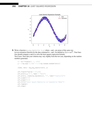
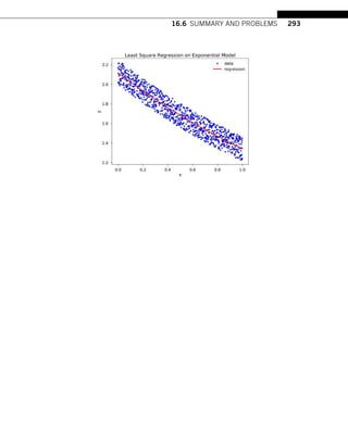
![296 CHAPTER 17 INTERPOLATION
coordinates of a car over time. Since motion is restricted to the maneuvering physics of the car, we can
expect that the points between the (x,y) coordinates in our set will be “smooth” rather than jagged.
The following sections will present several common interpolation methods.
17.2 LINEAR INTERPOLATION
In linear interpolation, the estimated point is assumed to lie on the line joining the nearest points to
the left and right. Assume, without loss of generality, that the x-data points are in ascending order, that
is, xi xi+1, and let x be a point such that xi x xi+1. Then the linear interpolation at x is
ŷ(x) = yi +
(yi+1 − yi)(x − xi)
(xi+1 − xi)
.
TRY IT! Find the linear interpolation at x = 1.5 based on the data x = [0, 1, 2], y = [1, 3,
2]. Verify the result using SciPy’s function interp1d.
Since 1 x 2, we use the second and third data points to compute the linear interpolation.
Plugging in the corresponding values gives
ŷ(x) = yi +
(yi+1 − yi)(x − xi)
(xi+1 − xi)
= 3 +
(2 − 3)(1.5 − 1)
(2 − 1)
= 2.5.
In [1]: from scipy.interpolate import interp1d
import matplotlib.pyplot as plt
plt.style.use(seaborn-poster)
In [2]: x = [0, 1, 2]
y = [1, 3, 2]
f = interp1d(x, y)
y_hat = f(1.5)
print(y_hat)
2.5
In [3]: plt.figure(figsize = (10,8))
plt.plot(x, y, -ob)
plt.plot(1.5, y_hat, ro)
plt.title(Linear Interpolation at x = 1.5)
plt.xlabel(x)](https://image.slidesharecdn.com/pythonprogrammingandnumericalmethodsaguideforengineersand-231017183839-0fbc5295/85/Python_Programming_and_Numerical_Methods_A_Guide_for_Engineers_and-pdf-302-320.jpg)
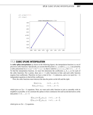
![298 CHAPTER 17 INTERPOLATION
Two more equations are required to compute the coefficients of Si(x). These last two constraints are
arbitrary; they can be chosen to fit the circumstances of the interpolation being performed. A common
set of final constraints is to assume that the second derivatives are zero at the endpoints. This means
that the curve is a “straight line” at the end points. Explicitly,
S
1 (x1) = 0,
S
n−1(xn) = 0.
In Python, we can use SciPy’s function CubicSpline to perform cubic spline interpolation. Note
that the above constraints are not the same as those used by SciPy’s CubicSpline as a default for
performing cubic splines. There are different ways to add the final two constraints in SciPy by setting
the bc_type argument (see help for CubicSpline to learn more).
TRY IT! Use CubicSpline to plot the cubic spline interpolation of the dataset x = [0, 1, 2]
and y = [1, 3, 2] for 0 ≤ x ≤ 2.
In [1]: from scipy.interpolate import CubicSpline
import numpy as np
import matplotlib.pyplot as plt
plt.style.use(seaborn-poster)
In [2]: x = [0, 1, 2]
y = [1, 3, 2]
# use bc_type = natural adds the constraints
f = CubicSpline(x, y, bc_type=natural)
x_new = np.linspace(0, 2, 100)
y_new = f(x_new)
In [3]: plt.figure(figsize = (10,8))
plt.plot(x_new, y_new, b)
plt.plot(x, y, ro)
plt.title(Cubic Spline Interpolation)
plt.xlabel(x)
plt.ylabel(y)
plt.show()](https://image.slidesharecdn.com/pythonprogrammingandnumericalmethodsaguideforengineersand-231017183839-0fbc5295/85/Python_Programming_and_Numerical_Methods_A_Guide_for_Engineers_and-pdf-304-320.jpg)
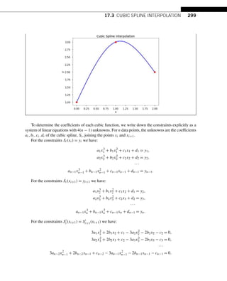
![300 CHAPTER 17 INTERPOLATION
For the constraints S
i (xi+1) = S
i+1(xi+1) we have:
6a1x2 + 2b1 − 6a2x2 − 2b2 = 0,
6a2x3 + 2b2 − 6a3x3 − 2b3 = 0,
...
6an−2xn−1 + 2bn−2 − 6an−1xn−1 − 2bn−1 = 0.
Finally, for the endpoint constraints S
1 (x1) = 0 and S
n−1(xn) = 0, we have:
6a1x1 + 2b1 = 0,
6an−1xn + 2bn−1 = 0.
These equations are linear in the unknown coefficients ai,bi,ci, and di. We can put them in matrix
form and solve for the coefficients of each spline by left division. Remember that whenever we solve
the matrix equation Ax = b for x, we must make sure that A is square and invertible. In the case of
finding cubic spline equations, the A matrix is always square and invertible as long as the xi values in
the dataset are unique.
TRY IT! Find the cubic spline interpolation at x = 1.5 based on the data x = [0, 1, 2], y =
[1, 3, 2].
First, we create the appropriate system of equations and find the coefficients of the cubic
splines by solving the system in matrix form.
The matrix form of the system of equations is
⎡
⎢
⎢
⎢
⎢
⎢
⎢
⎢
⎢
⎢
⎢
⎣
0 0 0 1 0 0 0 0
0 0 0 0 1 1 1 1
1 1 1 1 0 0 0 0
0 0 0 0 8 4 2 1
3 2 1 0 −3 −2 −1 0
6 2 0 0 −6 −2 0 0
0 2 0 0 0 0 0 0
0 0 0 0 12 2 0 0
⎤
⎥
⎥
⎥
⎥
⎥
⎥
⎥
⎥
⎥
⎥
⎦
⎡
⎢
⎢
⎢
⎢
⎢
⎢
⎢
⎢
⎢
⎢
⎣
a1
b1
c1
d1
a2
b2
c2
d2
⎤
⎥
⎥
⎥
⎥
⎥
⎥
⎥
⎥
⎥
⎥
⎦
=
⎡
⎢
⎢
⎢
⎢
⎢
⎢
⎢
⎢
⎢
⎢
⎣
1
3
3
2
0
0
0
0
⎤
⎥
⎥
⎥
⎥
⎥
⎥
⎥
⎥
⎥
⎥
⎦
.
In [4]: b = np.array([1, 3, 3, 2, 0, 0, 0, 0])
b = b[:, np.newaxis]
A = np.array([[0, 0, 0, 1, 0, 0, 0, 0],
[0, 0, 0, 0, 1, 1, 1, 1],
[1, 1, 1, 1, 0, 0, 0, 0],
[0, 0, 0, 0, 8, 4, 2, 1],
[3, 2, 1, 0, -3, -2, -1, 0],
[6, 2, 0, 0, -6, -2, 0, 0],
[0, 2, 0, 0, 0, 0, 0, 0],
[0, 0, 0, 0, 12, 2, 0, 0]])](https://image.slidesharecdn.com/pythonprogrammingandnumericalmethodsaguideforengineersand-231017183839-0fbc5295/85/Python_Programming_and_Numerical_Methods_A_Guide_for_Engineers_and-pdf-306-320.jpg)
![17.4 LAGRANGE POLYNOMIAL INTERPOLATION 301
In [5]: np.dot(np.linalg.inv(A), b)
Out[5]: array([[-0.75],
[ 0. ],
[ 2.75],
[ 1. ],
[ 0.75],
[-4.5 ],
[ 7.25],
[-0.5 ]])
The two cubic polynomials are
S1(x) = −0.75x3
+ 2.75x + 1 for 0 ≤ x ≤ 1, and (17.1)
S2(x) = 0.75x3
− 4.5x2
+ 7.25x − 0.5 for 1 ≤ x ≤ 2. (17.2)
So for x = 1.5, we evaluate S2(1.5) and obtain an estimated value of 2.7813.
17.4 LAGRANGE POLYNOMIAL INTERPOLATION
Rather than finding cubic polynomials between subsequent pairs of data points, Lagrange polynomial
interpolation finds a single polynomial that goes through all the data points. This polynomial is re-
ferred to as a Lagrange polynomial, L(x). As an interpolation function, it should have the property
L(xi) = yi for every point in the dataset. When computing Lagrange polynomials, it is useful to write
them as a linear combination of Lagrange basis polynomials, Pi(x), where
Pi(x) =
n
j=1,j=i
x − xj
xi − xj
,
and
L(x) =
n
i=1
yiPi(x).
Here, means “the product of” or “multiply out.” Note that, by construction, Pi(x) has the property
that Pi(xj ) = 1 when i = j and Pi(xj ) = 0 when i = j. Since L(x) is a sum of these polynomials,
observe that L(xi) = yi for every point, exactly as desired.](https://image.slidesharecdn.com/pythonprogrammingandnumericalmethodsaguideforengineersand-231017183839-0fbc5295/85/Python_Programming_and_Numerical_Methods_A_Guide_for_Engineers_and-pdf-307-320.jpg)
![302 CHAPTER 17 INTERPOLATION
TRY IT! Find the Lagrange basis polynomials for the dataset x = [0,1,2] and y = [1,3,2]. Plot
each polynomial and verify the property that Pi(xj ) = 1 when i = j and Pi(xj ) = 0 when i = j.
P1(x) =
(x − x2)(x − x3)
(x1 − x2)(x1 − x3)
=
(x − 1)(x − 2)
(0 − 1)(0 − 2)
=
1
2
(x2
− 3x + 2),
P2(x) =
(x − x1)(x − x3)
(x2 − x1)(x2 − x3)
=
(x − 0)(x − 2)
(1 − 0)(1 − 2)
= −x2
+ 2x,
P3(x) =
(x − x1)(x − x2)
(x3 − x1)(x3 − x2)
=
(x − 0)(x − 1)
(2 − 0)(2 − 1)
=
1
2
(x2
− x).
In [1]: import numpy as np
import numpy.polynomial.polynomial as poly
import matplotlib.pyplot as plt
plt.style.use(seaborn-poster)
In [2]: x = [0, 1, 2]
y = [1, 3, 2]
P1_coeff = [1,-1.5,.5]
P2_coeff = [0, 2,-1]
P3_coeff = [0,-.5,.5]
# get the polynomial function
P1 = poly.Polynomial(P1_coeff)
P2 = poly.Polynomial(P2_coeff)
P3 = poly.Polynomial(P3_coeff)
x_new = np.arange(-1.0, 3.1, 0.1)
fig = plt.figure(figsize = (10,8))
plt.plot(x_new, P1(x_new), b, label = P1)
plt.plot(x_new, P2(x_new), r, label = P2)
plt.plot(x_new, P3(x_new), g, label = P3)
plt.plot(x, np.ones(len(x)), ko, x,np.zeros(len(x)), ko)
plt.title(Lagrange Basis Polynomials)
plt.xlabel(x)
plt.ylabel(y)
plt.grid()
plt.legend()
plt.show()](https://image.slidesharecdn.com/pythonprogrammingandnumericalmethodsaguideforengineersand-231017183839-0fbc5295/85/Python_Programming_and_Numerical_Methods_A_Guide_for_Engineers_and-pdf-308-320.jpg)
![17.4 LAGRANGE POLYNOMIAL INTERPOLATION 303
TRY IT! Using the previous example, compute and plot the Lagrange polynomial. Verify that it
goes through each of the data points.
In [3]: L = P1 + 3*P2 + 2*P3
fig = plt.figure(figsize = (10,8))
plt.plot(x_new, L(x_new), b, x, y, ro)
plt.title(Lagrange Polynomial)
plt.grid()
plt.xlabel(x)
plt.ylabel(y)
plt.show()](https://image.slidesharecdn.com/pythonprogrammingandnumericalmethodsaguideforengineersand-231017183839-0fbc5295/85/Python_Programming_and_Numerical_Methods_A_Guide_for_Engineers_and-pdf-309-320.jpg)
![304 CHAPTER 17 INTERPOLATION
WARNING! Lagrange interpolation polynomials are defined outside the area of interpolation,
that is, outside of the interval [x1,xn], and will grow very fast and unbounded outside this region.
This is not a desirable feature because, in general, this does not agree with the behavior of the
underlying data. Thus, Lagrange interpolation should be used with caution outside the region of
interest.
17.4.1 USING THE LAGRANGE FUNCTION FROM SCIPY
Instead of calculating everything from scratch, in SciPy we can use the lagrange function directly to
interpolate the data. Let us use the above example to illustrate our point.
In [4]: from scipy.interpolate import lagrange
In [5]: f = lagrange(x, y)
In [6]: fig = plt.figure(figsize = (10,8))
plt.plot(x_new, f(x_new), b, x, y, ro)
plt.title(Lagrange Polynomial)
plt.grid()
plt.xlabel(x)
plt.ylabel(y)
plt.show()](https://image.slidesharecdn.com/pythonprogrammingandnumericalmethodsaguideforengineersand-231017183839-0fbc5295/85/Python_Programming_and_Numerical_Methods_A_Guide_for_Engineers_and-pdf-310-320.jpg)
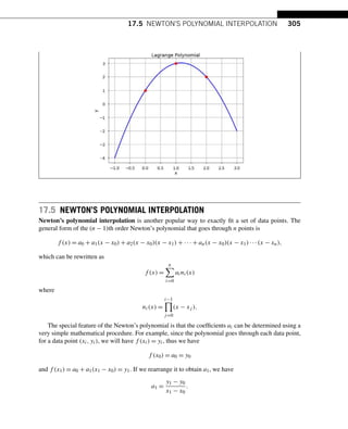
![306 CHAPTER 17 INTERPOLATION
If we insert data point (x2,y2), we can calculate a2, and it becomes
a2 =
y2−y1
x2−x1
− y1−y0
x1−x0
x2 − x0
.
Let us do one more data point (x3,y3) to calculate a3. After inserting the data point into the equa-
tion, we obtain
a3 =
y3−y2
x3−x2
−
y2−y1
x2−x1
x3−x1
−
y2−y1
x2−x1
−
y1−y0
x1−x0
x2−x0
x3 − x0
.
See the patterns? These are called divided differences. If we define
f [x1,x0] =
y1 − y0
x1 − x0
,
then
f [x2,x1,x0] =
y2−y1
x2−x1
− y1−y0
x1−x0
x2 − x0
=
f [x2,x1] − f [x1,x0]
x2 − x1
.
If we continue write this out, we will obtain the following iteration equation:
f [xk,xk−1,...,x1,x0] =
f [xk,xk−1,...,x2,x2] − f [xk−1,xk−2,...,x1,x0]
xk − x0
.
The advantage of using this method is that once the coefficients are determined, adding new data
points will not change the previously calculated coefficient; we only need to calculate the higher dif-
ferences in the same manner. The whole procedure for finding these coefficients can be summarized
into a divided difference table. An example using five data points is shown below:
x0 y0
f [x1,x0]
x1 y1 f [x2,x1,x0]
f [x2,x1] f [x3,x2,x1,x0]
x2 y2 f [x3,x2,x1] f [x4,x3,x2,x1,x0]
f [x3,x2] f [x4,x3,x2,x1]
x3 y3 f [x4,x3,x2]
f [x4,x3]
x4 y4
Each element in the table can be calculated using the two previous elements (to the left). In reality,
we can calculate all elements and store them in a diagonal matrix–that is, as the coefficient matrix–](https://image.slidesharecdn.com/pythonprogrammingandnumericalmethodsaguideforengineersand-231017183839-0fbc5295/85/Python_Programming_and_Numerical_Methods_A_Guide_for_Engineers_and-pdf-312-320.jpg)
![17.5 NEWTON’S POLYNOMIAL INTERPOLATION 307
which can be written as
y0 f [x1,x0] f [x2,x1,x0] f [x3,x2,x1,x0] f [x4,x3,x2,x1,x0]
y1 f [x2,x1] f [x3,x2,x1] f [x4,x3,x2,x1] 0
y2 f [x3,x2] f [x4,x3,x2] 0 0
y3 f [x4,x3] 0 0 0
y4 0 0 0 0
Note that the first row in the matrix is actually all the coefficients that we need, i.e., a0,a1,a2,a3,
and a4. Shown below is an example of how to do this.
TRY IT! Calculate the divided difference table for x = [-5, -1, 0, 2], y = [-2, 6, 1, 3].
In [1]: import numpy as np
import matplotlib.pyplot as plt
plt.style.use(seaborn-poster)
%matplotlib inline
In [2]: def divided_diff(x, y):
function to calculate the divided
difference table
n = len(y)
coef = np.zeros([n, n])
# the first column is y
coef[:,0] = y
for j in range(1,n):
for i in range(n-j):
coef[i][j] = (coef[i+1][j-1]-coef[i][j-1])/(x[i+j]-x[i])
return coef
def newton_poly(coef, x_data, x):
evaluate the Newton polynomial
at x
n = len(x_data) - 1
p = coef[n]](https://image.slidesharecdn.com/pythonprogrammingandnumericalmethodsaguideforengineersand-231017183839-0fbc5295/85/Python_Programming_and_Numerical_Methods_A_Guide_for_Engineers_and-pdf-313-320.jpg)
![308 CHAPTER 17 INTERPOLATION
for k in range(1,n+1):
p = coef[n-k] + (x -x_data[n-k])*p
return p
In [3]: x = np.array([-5, -1, 0, 2])
y = np.array([-2, 6, 1, 3])
# get the divided difference coef
a_s = divided_diff(x, y)[0, :]
# evaluate on new data points
x_new = np.arange(-5, 2.1, .1)
y_new = newton_poly(a_s, x, x_new)
plt.figure(figsize = (12, 8))
plt.plot(x, y, bo)
plt.plot(x_new, y_new)
Out[3]: [matplotlib.lines.Line2D at 0x11bd4e630]
We can see that the Newton’s polynomial goes through all the data points and fits the data.
17.6 SUMMARY AND PROBLEMS
17.6.1 SUMMARY
1. Given a set of reliable data points, interpolation is a method of estimating dependent variable values
for independent variable values not in the dataset.
2. Linear, Cubic Spline, Lagrange, and Newton’s polynomial interpolation are common interpolation
methods.](https://image.slidesharecdn.com/pythonprogrammingandnumericalmethodsaguideforengineersand-231017183839-0fbc5295/85/Python_Programming_and_Numerical_Methods_A_Guide_for_Engineers_and-pdf-314-320.jpg)
![17.6 SUMMARY AND PROBLEMS 309
17.6.2 PROBLEMS
1. Write a function my_lin_interp(x, y, X) where x and y are arrays that contain experimental data
points, and X is an array. Assume that x and X are in ascending order and have unique elements. The
output argument, Y, should be an array the same size as X, where Y[i] is the linear interpolation of
X[i]. Do not use interp from NumPy or interp1d from SciPy.
2. Write a function my_cubic_spline(x, y, X) where x and y are arrays that contain experimental
data points, and X is an array. Assume that x and X are in ascending order and have unique ele-
ments. The output argument, Y, should be an array the same size as X, where Y[i] is cubic spline
interpolation of X[i]. Do not use interp1d or CubicSpline.
3. Write a function my_nearest_neighbor(x, y, X) where x and y are arrays that contain experi-
mental data points, and X is an array. Assume that x and X are in ascending order and have unique
elements. The output argument, Y, should be an array the same size as X, where Y[i] is the near-
est neighbor interpolation of X[i]. That is, Y[i] should be the y[j] where x[j] is the closest
independent data point of X[i]. Do not use interp1d from SciPy.
4. Think of a circumstance where using the nearest neighbor interpolation would be superior to cubic
spline interpolation.
5. Write a function my_cubic_spline_flat(x, y, X) where x and y are arrays that contain experi-
mental data points, and X is an array. Assume that x and X are in ascending order and have unique
elements. The output argument, Y, should be an array the same size as X, where Y[i] is the cubic
spline interpolation of X[i]. Instead of the constraints introduced previously, use S
1(x1) = 0 and
S
n−1(xn) = 0.
6. Write a function my_quintic_spline(x, y, X) where x and y are arrays that contain experimental
data points, and X is an array. Assume that x and X are in ascending order and have unique elements.
The output argument, Y, should be an array the same size as X, where Y[i] is the quintic spline
interpolation of X[i]. You will need to use additional endpoint constraints to come up with enough
constraints. You may use endpoint constraints at your discretion.
7. Write a function my_interp_plotter(x, y, X, option) where x and y are arrays containing
experimental data points, and X is an array that contains the coordinates for which an interpolation
is desired. The input argument option should be a string, either “linear,” “spline,” or “nearest.”
Your function should produce a plot of the data points (x,y) marked as red circles. The points
(X,Y), where X is the input and Y is the interpolation at the points contained in X defined by the
input argument specified by option. The points (X,Y) should be connected by a blue line. Be sure
to include the title, axis labels, and a legend. Hint: You should use interp1d from SciPy, and
checkout the kind option.
Test cases:
x = np.array([0, .1, .15, .35, .6, .7, .95, 1])
y=np.array([1,0.8187,0.7408,0.4966,0.3012,0.2466,0.1496,0.1353])
my_interp_plotter(x, y, np.linspace(0, 1, 101), nearest)](https://image.slidesharecdn.com/pythonprogrammingandnumericalmethodsaguideforengineersand-231017183839-0fbc5295/85/Python_Programming_and_Numerical_Methods_A_Guide_for_Engineers_and-pdf-315-320.jpg)
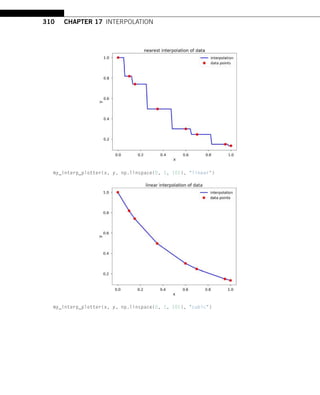
![17.6 SUMMARY AND PROBLEMS 311
8. Write a function my_D_cubic_spline(x, y, X, D), where the output Y is the cubic spline in-
terpolation at X taken from the data points contained in x and y. Instead of the standard pinned
endpoint conditions (i.e., S
1 (x1) = 0 and S
n−1(xn) = 0), use the endpoint conditions S
1(x1) = D
and S
n−1(xn) = D (i.e., the slopes of the interpolating polynomials at the endpoints are D).
Test cases:
x = [0, 1, 2, 3, 4]
y = [0, 0, 1, 0, 0]
X = np.linspace(0, 4, 101)
# Solution: Y = 0.54017857
Y = my_D_cubic_spline(x, y, 1.5, 1)
plt.figure(figsize = (10, 8))
plt.subplot(221)
plt.plot(x, y, ro, X, my_D_cubic_spline(x, y, X, 0), b)
plt.subplot(222)
plt.plot(x, y, ro, X, my_D_cubic_spline(x, y, X, 1), b)
plt.subplot(223)
plt.plot(x, y, ro, X, my_D_cubic_spline(x, y, X, -1), b)
plt.subplot(224)
plt.plot(x, y, ro, X, my_D_cubic_spline(x, y, X, 4), b)
plt.tight_layout()
plt.show()](https://image.slidesharecdn.com/pythonprogrammingandnumericalmethodsaguideforengineersand-231017183839-0fbc5295/85/Python_Programming_and_Numerical_Methods_A_Guide_for_Engineers_and-pdf-317-320.jpg)
![312 CHAPTER 17 INTERPOLATION
9. Write a function my_lagrange(x, y, X) where the output Y is the Lagrange interpolation of the
data points contained in x and y computed at X. Hint: Use a nested for-loop, where the inner
for-loop computes the product for the Lagrange basis polynomial and the outer loop computes the
sum for the Lagrange polynomial. Don’t use the existing lagrange function from SciPy.
Test cases:
x = [0, 1, 2, 3, 4]
y = [2, 1, 3, 5, 1]
X = np.linspace(0, 4, 101)
plt.figure(figsize = (10,8 ))
plt.plot(X, my_lagrange(x, y, X), b, label = interpolation)
plt.plot(x, y, ro, label = data points)
plt.xlabel(x)
plt.ylabel(y)
plt.title(fLagrange Interpolation of Data Points)
plt.legend()
plt.show()](https://image.slidesharecdn.com/pythonprogrammingandnumericalmethodsaguideforengineersand-231017183839-0fbc5295/85/Python_Programming_and_Numerical_Methods_A_Guide_for_Engineers_and-pdf-318-320.jpg)
![17.6 SUMMARY AND PROBLEMS 313
10. Fit the data x = [0, 1, 2, 3, 4], y = [2, 1, 3, 5, 1] using Newton’s polynomial interpolation.](https://image.slidesharecdn.com/pythonprogrammingandnumericalmethodsaguideforengineersand-231017183839-0fbc5295/85/Python_Programming_and_Numerical_Methods_A_Guide_for_Engineers_and-pdf-319-320.jpg)
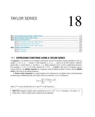
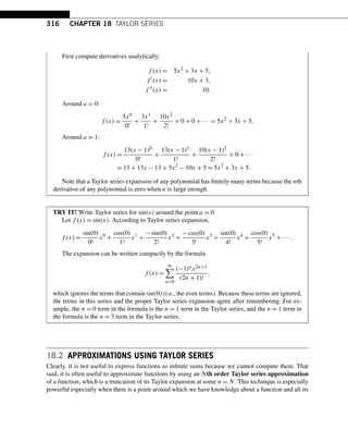
![18.2 APPROXIMATIONS USING TAYLOR SERIES 317
derivatives. For example, if we take the Taylor expansion of ex around a = 0, then f (n)(a) = 1 for all
n, and we do not have to compute the derivatives in the Taylor expansion to approximate ex!
TRY IT! Use Python to plot the sin function along with the first, third, fifth, and seventh order
Taylor series approximations. Note that this involves the zeroth to third terms in the formula given
earlier.
In [1]: import numpy as np
import matplotlib.pyplot as plt
plt.style.use(seaborn-poster)
In [2]: x = np.linspace(-np.pi, np.pi, 200)
y = np.zeros(len(x))
labels = [First Order, Third Order,
Fifth Order, Seventh Order]
plt.figure(figsize = (10,8))
for n, label in zip(range(4), labels):
y=y+((-1)**n*(x)**(2*n+1))/np.math.factorial(2*n+1)
plt.plot(x,y, label = label)
plt.plot(x, np.sin(x), k, label = Analytic)
plt.grid()
plt.title(Taylor Series Approximations of Various Orders)
plt.xlabel(x)
plt.ylabel(y)
plt.legend()
plt.show()](https://image.slidesharecdn.com/pythonprogrammingandnumericalmethodsaguideforengineersand-231017183839-0fbc5295/85/Python_Programming_and_Numerical_Methods_A_Guide_for_Engineers_and-pdf-322-320.jpg)
![318 CHAPTER 18 TAYLOR SERIES
Obviously, the approximation approaches the analytic function quickly, even for x not near a = 0.
Note that in the above code, we also used a new function zip, which allows us to loop through two
parameters range(4) and labels to use in our plot.
TRY IT! Compute the seventh order Taylor series approximation for sin(x) around a = 0 at
x = π/2. Compare the value to the correct value, 1.
In [3]: x = np.pi/2
y = 0
for n in range(4):
y=y+((-1)**n *(x)**(2*n+1))/np.math.factorial(2*n+1)
print(y)
0.9998431013994987
The seventh order Taylor series approximation is very close to the theoretical value of the function
even if it is computed far from the point around which the Taylor series was computed (i.e., x = π/2
and a = 0).
The most common Taylor series approximation is the first order approximation, or linear approxi-
mation. Intuitively, for “smooth” functions the linear approximation of the function around a point, a,
is legitimate provided you stay sufficiently close to a. In other words, “smooth” functions look more
and more like a line the more you zoom into any point. In the figure below this has been plotted in
successive levels of zoom using a smooth function to illustrate the linear nature of functions locally.
Linear approximations are useful tools when analyzing “complicated” functions locally.](https://image.slidesharecdn.com/pythonprogrammingandnumericalmethodsaguideforengineersand-231017183839-0fbc5295/85/Python_Programming_and_Numerical_Methods_A_Guide_for_Engineers_and-pdf-323-320.jpg)
![18.2 APPROXIMATIONS USING TAYLOR SERIES 319
In [4]: x = np.linspace(0, 3, 30)
y = np.exp(x)
plt.figure(figsize = (14, 4.5))
plt.subplot(1, 3, 1)
plt.plot(x, y)
plt.grid()
plt.subplot(1, 3, 2)
plt.plot(x, y)
plt.grid()
plt.xlim(1.7, 2.3)
plt.ylim(5, 10)
plt.subplot(1, 3, 3)
plt.plot(x, y)
plt.grid()
plt.xlim(1.92, 2.08)
plt.ylim(6.6, 8.2)
plt.tight_layout()
plt.show()
TRY IT! Take the linear approximation for ex around point a = 0. Use the linear approximation
for ex to approximate the value of e1 and e0.01. Use the NumPy’s function exp to compute exp(1)
and exp(0.01) and compare the results.
The linear approximation of ex around a = 0 is 1 + x.
The NumPy’s exp function gives the following:
In [5]: np.exp(1)
Out[5]: 2.718281828459045
In [6]: np.exp(0.01)
Out[6]: 1.010050167084168](https://image.slidesharecdn.com/pythonprogrammingandnumericalmethodsaguideforengineersand-231017183839-0fbc5295/85/Python_Programming_and_Numerical_Methods_A_Guide_for_Engineers_and-pdf-324-320.jpg)
![320 CHAPTER 18 TAYLOR SERIES
The linear approximation of e1 is 2, which is inaccurate, and the linear approximation of e0.01 is
1.01, which is very good. This example illustrates how the linear approximation becomes close to the
point from which the approximation is taken.
18.3 DISCUSSION ABOUT ERRORS
18.3.1 TRUNCATION ERRORS FOR TAYLOR SERIES
In numerical analysis, there are usually two sources of error, round-off and truncation. The round-off
errors are due to the inexactness in the representation of real numbers on a computer and the arithmetic
operations performed with them. Refer to Chapter 9 for additional discussion on this type of error.
The truncation errors are due to the approximate nature of the method used and usually arise when
using an approximation in place of an exact mathematical procedure, e.g., when we used Taylor series
to approximate a function. For example, if we use Taylor series to approximate the function ex, we
obtain
ex
= 1 + x +
x2
2!
+
x3
3!
+
x4
4!
+ ··· .
Since it takes an infinite sequence to approximate the function, using only a few terms will result in
an approximation (or truncation) error. For example, if we only use the first four terms to approximate
e2, we obtain
e2
≈ 1 + 2 +
22
2!
+
23
3!
= 6.3333.
There is obviously an error associated with such a solution, since we truncated the rest of the terms
in the Taylor series. Therefore the function f (x) can be written as the Taylor series approximation plus
a truncation error term
f (x) = fn(x) + En(x).
The more terms we use, the closer the approximation will be to the exact value. Let us use Python
to calculate the above example.
TRY IT! Approximate e2 using different order Taylor series and print out the results.
In [1]: import numpy as np
In [2]: exp = 0
x = 2
for i in range(10):
exp = exp + (x**i)/np.math.factorial(i)
print(fUsing {i}-term, {exp})](https://image.slidesharecdn.com/pythonprogrammingandnumericalmethodsaguideforengineersand-231017183839-0fbc5295/85/Python_Programming_and_Numerical_Methods_A_Guide_for_Engineers_and-pdf-325-320.jpg)
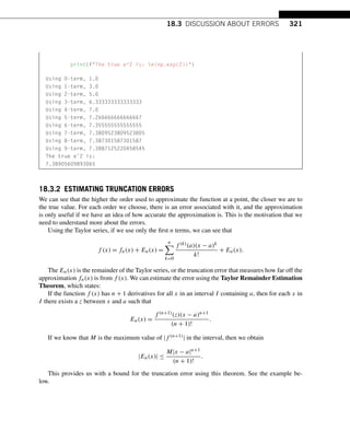
![322 CHAPTER 18 TAYLOR SERIES
TRY IT! Estimate the remainder bound for the approximation using Taylor series for e2 using
n = 9.
To understand the basis of this error, when we use n = 9, we know that (ex) = ex, and a = 0;
therefore, the error related to x = 2 is
En(x) =
f (9+1)(z)(x)(9+1)
(9 + 1)!
=
ez210
10!
.
Recall that 0 ≤ z ≤ 2, and e 3; therefore,
|En(x)| ≤
32210
10!
= 0.00254.
If we use Taylor series with n = 9 to approximate e2, our absolute error should be less than
0.00254. We verify this below.
In [3]: abs(7.3887125220458545-np.exp(2))
Out[3]: 0.0003435768847959153
18.3.3 ROUND-OFF ERRORS FOR TAYLOR SERIES
Numerically, when adding many terms in a sum, we should be mindful of numerical accumulation of
errors that is due to floating point round-off errors; see the following example.
EXAMPLE: Approximate e−30 using different order Taylor series, and print out the results.
In [4]: exp = 0
x = -30
for i in range(200):
exp = exp + (x**i)/np.math.factorial(i)
print(fUsing {i}-term, our result is {exp})
print(fThe true e^2 is: {np.exp(x)})
Using 199-term, our result is -8.553016433669241e-05
The true eˆ2 is: 9.357622968840175e-14
From the above example, it is clear that our estimation using Taylor series is not close to the true
value anymore, no matter how many terms we include into the calculation, which is due to the round-off
errors we discussed earlier. To obtain a small result, when using negative large arguments, the Taylor
series requires alternating large numbers to cancel out. We need many digits for precision in the series
to capture both the large and small numbers with enough remaining digits to get the result in the desired
output precision. This is why the program threw an error message in the example above.](https://image.slidesharecdn.com/pythonprogrammingandnumericalmethodsaguideforengineersand-231017183839-0fbc5295/85/Python_Programming_and_Numerical_Methods_A_Guide_for_Engineers_and-pdf-327-320.jpg)
![19
ROOT FINDING
19.1 Root Finding Problem Statement.................................................................................. 325
19.2 Tolerance ............................................................................................................. 326
19.3 Bisection Method.................................................................................................... 327
19.4 Newton–Raphson Method .......................................................................................... 330
19.5 Root Finding in Python.............................................................................................. 332
19.6 Summary and Problems ............................................................................................ 333
19.6.1 Summary............................................................................................ 333
19.6.2 Problems ............................................................................................ 333
19.1 ROOT FINDING PROBLEM STATEMENT
The root or zero of a function, f (x), is an xr such that f (xr) = 0. For functions such as f (x) = x2 − 9,
the roots are clearly 3 and −3. However, for other functions, such as f (x) = cos(x) − x, determining
an analytic or exact solution for the roots of functions can be difficult. For these cases, it is useful to
generate numerical approximations of the roots of f and understand their limitations.
TRY IT! Use the fsolve function from SciPy to compute the root of f (x) = cos(x) − x near
−2. Verify that the solution is a root (or close enough).
In [1]: import numpy as np
from scipy import optimize
f = lambda x: np.cos(x) - x
r = optimize.fsolve(f, -2)
print(r =, r)
# Verify the solution is a root
result = f(r)
print(result=, result)
r = [0.73908513]
result= [0.]](https://image.slidesharecdn.com/pythonprogrammingandnumericalmethodsaguideforengineersand-231017183839-0fbc5295/85/Python_Programming_and_Numerical_Methods_A_Guide_for_Engineers_and-pdf-329-320.jpg)
![326 CHAPTER 19 ROOT FINDING
TRY IT! The function f (x) = 1
x has no root. Use the fsolve function to try to compute the root
of f (x) = 1
x . Turn on the full_output to see what is going on. Check the documentation for
details.
In [2]: f = lambda x: 1/x
r, infodict, ier, mesg =
optimize.fsolve(f, -2, full_output=True)
print(r =, r)
result = f(r)
print(result=, result)
print(mesg)
r = [-3.52047359e+83]
result= [-2.84052692e-84]
The number of calls to function has reached maxfev = 400.
The value r that was returned is not a root, even though the value of f (r) is a very small number.
Since we turned on the full_output, we can see more information. A message would have been
returned if no solution was found; we can see mesg details for the cause of failure: “The number of
calls to function has reached maxfev = 400.”
19.2 TOLERANCE
In engineering and science, error is a deviation from an expected or computed value. Tolerance is
the level of error that is acceptable for an engineering application. We say that a computer program
has converged to a solution when it has found a solution with an error smaller than the tolerance.
When computing roots numerically, or conducting any other kind of numerical analysis, it is important
to establish both a metric for error and a tolerance that is suitable for a given engineering/science
application.
For computing roots, we want an xr such that f (xr) is very close to zero. Therefore |f (x)| is a
possible choice for the measure of error since the smaller it is, the likelier we are to a root. Also, if we
assume that xi is the ith guess of an algorithm for finding a root, then |xi+1 − xi| is another possible
choice for measuring the error since we expect improvement between subsequent guesses to diminish
as it approaches a solution. As will be demonstrated in the following examples, these different choices
have their advantages and disadvantages.](https://image.slidesharecdn.com/pythonprogrammingandnumericalmethodsaguideforengineersand-231017183839-0fbc5295/85/Python_Programming_and_Numerical_Methods_A_Guide_for_Engineers_and-pdf-330-320.jpg)
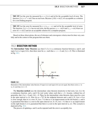
![328 CHAPTER 19 ROOT FINDING
FIGURE 19.2
Illustration of the bisection method. The sign of f (m) is checked to determine if the root is contained in the interval
(a,m) or (m,b). This new interval is used in the next iteration of the bisection method; in the case depicted in the
figure, the root is in the interval (m,b).
TRY IT! Program a function my_bisection(f,a,b,tol) that approximates a root r of f, bounded
by a and b to within |f (a+b
2 )| tol.
In [1]: import numpy as np
def my_bisection(f, a, b, tol):
# approximates a root, R, of f bounded
# by a and b to within tolerance
# | f(m) | tol with m being the midpoint
# between a and b. Recursive implementation
# check if a and b bound a root
if np.sign(f(a)) == np.sign(f(b)):
raise Exception(
The scalars a and b do not bound a root)
# get midpoint
m = (a + b)/2
if np.abs(f(m)) tol:
# stopping condition, report m as root
return m
elif np.sign(f(a)) == np.sign(f(m)):
# case where m is an improvement on a.
# Make recursive call with a = m
return my_bisection(f, m, b, tol)](https://image.slidesharecdn.com/pythonprogrammingandnumericalmethodsaguideforengineersand-231017183839-0fbc5295/85/Python_Programming_and_Numerical_Methods_A_Guide_for_Engineers_and-pdf-332-320.jpg)
![19.3 BISECTION METHOD 329
elif np.sign(f(b)) == np.sign(f(m)):
# case where m is an improvement on b.
# Make recursive call with b = m
return my_bisection(f, a, m, tol)
TRY IT! The
√
2 can be computed as the root of the function f (x) = x2 − 2. Starting at a = 0 and
b = 2, use my_bisection to approximate the
√
2 to a tolerance of |f (x)| 0.1 and |f (x)| 0.01.
Verify that the results are close to a root by plugging the root back into the function.
In [2]: f = lambda x: x**2 - 2
r1 = my_bisection(f, 0, 2, 0.1)
print(r1 =, r1)
r01 = my_bisection(f, 0, 2, 0.01)
print(r01 =, r01)
print(f(r1) =, f(r1))
print(f(r01) =, f(r01))
r1 = 1.4375
r01 = 1.4140625
f(r1) = 0.06640625
f(r01) = -0.00042724609375
TRY IT! See what happens if you use a = 2 and b = 4 for the above function.
In [3]: my_bisection(f, 2, 4, 0.01)
--------------------------------------------------------
Exception Traceback (most recent call last)
ipython-input-3-4158b7a9ae67 in module
---- 1 my_bisection(f, 2, 4, 0.01)
ipython-input-1-36f06123e87c in my_bisection(f,a,b,tol)
10 if np.sign(f(a)) == np.sign(f(b)):
11 raise Exception(
--- 12 The scalars a and b do not bound a root)
13](https://image.slidesharecdn.com/pythonprogrammingandnumericalmethodsaguideforengineersand-231017183839-0fbc5295/85/Python_Programming_and_Numerical_Methods_A_Guide_for_Engineers_and-pdf-333-320.jpg)
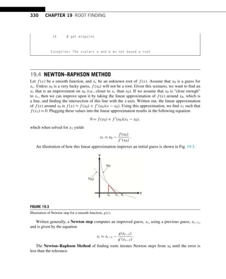
![19.4 NEWTON–RAPHSON METHOD 331
TRY IT! Again, the
√
2 is the root of the function f (x) = x2 − 2. Using x0 = 1.4 as a starting
point, use the previous equation to estimate
√
2. Compare this approximation with the value
computed by Python’s sqrt function.
x = 1.4 −
1.42 − 2
2(1.4)
= 1.4142857142857144.
In [1]: import numpy as np
f = lambda x: x**2 - 2
f_prime = lambda x: 2*x
newton_raphson = 1.4 - (f(1.4))/(f_prime(1.4))
print(newton_raphson =, newton_raphson)
print(sqrt(2) =, np.sqrt(2))
newton_raphson = 1.4142857142857144
sqrt(2) = 1.4142135623730951
TRY IT! Write a function my_newton(f,df,x0,tol) where the output is an estimate of the root
of f, f is a function object f (x), df is a function object f (x), x0 is an initial guess, and tol is
the error tolerance. The error measurement should be |f (x)|.
In [2]: def my_newton(f, df, x0, tol):
# output is an estimation of the root of f
# using the Newton-Raphson method
# recursive implementation
if abs(f(x0)) tol:
return x0
else:
return my_newton(f, df, x0 - f(x0)/df(x0), tol)
TRY IT! Use my_newton to compute
√
2 to within a tolerance of 1e-6 starting at x0 = 1.5.
In [3]: estimate = my_newton(f, f_prime, 1.5, 1e-6)
print(estimate =, estimate)
print(sqrt(2) =, np.sqrt(2))
estimate = 1.4142135623746899
sqrt(2) = 1.4142135623730951
If x0 is close to xr, then it can be proven that, in general, the Newton–Raphson method converges
to xr much faster than the bisection method; however, since xr is initially unknown, there is no way to](https://image.slidesharecdn.com/pythonprogrammingandnumericalmethodsaguideforengineersand-231017183839-0fbc5295/85/Python_Programming_and_Numerical_Methods_A_Guide_for_Engineers_and-pdf-335-320.jpg)
![332 CHAPTER 19 ROOT FINDING
know if the initial guess is close enough to the root to obtain this behavior unless some special infor-
mation about the function is known a priori (e.g., the function has a root close to x = 0). In addition
to this initialization problem, the Newton–Raphson method has other serious limitations. For example,
if the derivative at a guess is close to zero, then the Newton step will be very large and probably lead
far away from the root. Also, depending on the behavior of the function derivative between x0 and xr,
the Newton–Raphson method may converge to a different root than xr which may not be useful for the
engineering application being considered.
TRY IT! Compute a single Newton step to get an improved approximation of the root of the
function f (x) = x3 + 3x2 − 2x − 5 and initial guess x0 = 0.29.
In [4]: x0 = 0.29
x1 = x0-(x0**3+3*x0**2-2*x0-5)/(3*x0**2+6*x0-2)
print(x1 =, x1)
x1 = -688.4516883116648
Note that f (x0) = −0.0077 (is close to zero), and the error at x1 is approximately 324880000
(very large).
TRY IT! Consider the polynomial f (x) = x3 − 100x2 − x + 100. This polynomial has a root at
x = 1 and x = 100. Use the Newton–Raphson method to find a root of f starting at x0 = 0.
At x0 = 0,f (x0) = 100, and f (x) = −1, the Newton step gives x1 = 0 − 100
−1 = 100, which is
a root of f . Note that this root is much farther from the initial guess than the other root at x = 1,
and it may not be the root you wanted from an initial guess of zero.
19.5 ROOT FINDING IN PYTHON
Unsurprisingly, Python has root-finding functions. The function we will use to find roots is f_solve
from the scipy.optimize.
The f_solve function takes in many arguments (study the documentation for addition information),
but the most important two are: (1) the function that you want to find the root and (2) the initial guess.
TRY IT! Compute the root of the function f (x) = x3 − 100x2 − x + 100 using f_solve.
In [1]: from scipy.optimize import fsolve
In [2]: f = lambda x: x**3-100*x**2-x+100
fsolve(f, [2, 80])](https://image.slidesharecdn.com/pythonprogrammingandnumericalmethodsaguideforengineersand-231017183839-0fbc5295/85/Python_Programming_and_Numerical_Methods_A_Guide_for_Engineers_and-pdf-336-320.jpg)
![19.6 SUMMARY AND PROBLEMS 333
Out[2]: array([ 1., 100.])
19.6 SUMMARY AND PROBLEMS
19.6.1 SUMMARY
1. Roots are an important property of functions.
2. The bisection method is a way of finding roots based on divide-and-conquer. Although stable, it
might converge slowly compared to the Newton–Raphson method.
3. The Newton–Raphson method is a different way of finding roots based on an approximation of the
function. Although the Newton–Raphson method converges quickly and stops near to the actual
root, it can be unstable.
19.6.2 PROBLEMS
1. Write a function my_nth_root(x,n,tol) where x and tol are strictly positive scalars, and n is an
integer strictly greater than 1. The output argument, r, should be an approximation r = N
√
x, the
Nth root of x. This approximation should be computed by using the Newton–Raphson method to
find the root of the function f (y) = yN − x. The error metric should be |f (y)|.
2. Write a function my_fixed_point(f,g,tol,max_iter) where f and g are function objects, and
tol and max_iter are strictly positive scalars. The input argument, max_iter, is also an integer.
The output argument, X, should be a scalar satisfying |f (X) − g(X)| tol, that is, X is a point
that (almost) satisfies f (X) = g(X). To find X, you should use the bisection method with the error
metric, |F(m)| tol. The function my_fixed_point should “give up” after max_iter number of
iterations and return X = [] if this occurs.
3. Why does the bisection method fail for f (x) = 1/x with an error given by |b − a|? Hint: How does
f (x) violate the intermediate value theorem?
4. Write a function my_bisection(f,a,b,tol) that returns [R,E], where f is a function object, a and
b are scalars such that a b, and tol is a strictly positive scalar value. The function should return
an array, R, where R[i] is the estimation of the root of f defined by (a + b)/2 for the ith iteration
of the bisection method. Remember to include the initial estimate. The function should also return
an array, E, where E[i] is the value of |f (R[i])| for the ith iteration of the bisection method. The
function should terminate when E(i) tol. Assume that sign(f (a)) = sign(f (b)).
Clarification: The input a and b constitute the first iteration of bisection; therefore, R and E should
never be empty.
Test cases:
In: f = lambda x: x**2 - 2
[R, E] = my_bisection(f, 0, 2, 1e-1)
Out: R = [1, 1.5, 1.25, 1.375, 1.4375]
E = [1, 0.25, 0.4375, 0.109375, 0.06640625]](https://image.slidesharecdn.com/pythonprogrammingandnumericalmethodsaguideforengineersand-231017183839-0fbc5295/85/Python_Programming_and_Numerical_Methods_A_Guide_for_Engineers_and-pdf-337-320.jpg)
![334 CHAPTER 19 ROOT FINDING
In: f = lambda x: np.sin(x) - np.cos(x)
[R, E] = my_bisection(f, 0, 2, 1e-2)
Out: R = [1, 0.5, 0.75, 0.875, 0.8125, 0.78125]
E = [0.30116867893975674, 0.39815702328616975,
0.05005010885048666, 0.12654664407270177,
0.038323093040207645, 0.005866372111545948]
5. Write a function my_newton(f,df,x0,tol) that returns [R,E], where f is a function object, df is a
function object giving the derivative of f, x0 is an initial estimation of the root, and tol is a strictly
positive scalar. The function should return an array, R, where R[i] is the Newton–Raphson estimate
of the root of f for the ith iteration. Remember to include the initial estimate. The function should
also return an array, E, where E[i] is the value of |f (R[i])| for the ith iteration of the Newton–
Raphson method. The function should terminate when E(i) tol. Assume that the derivative of
f will not hit zero during any iteration for any of the test cases given.
Test cases:
In: f = lambda x: x**2 - 2
df = lambda x: 2*x
[R, E] = my_newton(f, df, 1, 1e-5)
Out: R = [1, 1.5, 1.4166666666666667, 1.4142156862745099]
E = [1, 0.25, 0.006944444444444642, 6.007304882871267e-06]
In: f = lambda x: np.sin(x) - np.cos(x)
df = lambda x: np.cos(x) + np.sin(x)
[R, E] = my_newton(f, df, 1, 1e-5)
Out: R = [1, 0.782041901539138, 0.7853981759997019]
E = [0.30116867893975674, 0.004746462127804163,
1.7822277875723103e-08]
6. Consider the problem of building a pipeline from an offshore oil platform, a distance H miles from
the shoreline, to an oil refinery station on land, a distance L miles along the shore. The cost of
building the pipe is Cocean/mile while the pipe is under the ocean, and Cland/mile while the pipe is on
land. The pipe will be built in a straight line toward the shore where it will make contact at some
point, x, between 0 and L. It will continue along the shore on land until it reaches the oil refinery.
See the following figure for clarification.
Write a function my_pipe_builder(C_ocean,C_land,L,H) where the input arguments are as de-
scribed earlier, and x is the x-value that minimizes the total cost of the pipeline. Use the bisection
method to determine this value to within a tolerance of 1 × 10⁻⁶, starting at an initial bound of
a = 0 and b = L.
Test cases:
In: my_pipe_builder(20, 10, 100, 50)
Out: 28.867512941360474
In: my_pipe_builder(30, 10, 100, 50)
Out: 17.677670717239380](https://image.slidesharecdn.com/pythonprogrammingandnumericalmethodsaguideforengineersand-231017183839-0fbc5295/85/Python_Programming_and_Numerical_Methods_A_Guide_for_Engineers_and-pdf-338-320.jpg)
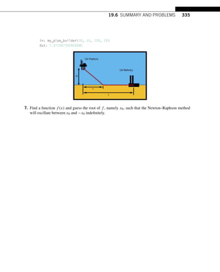
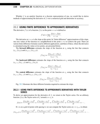
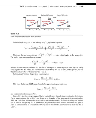
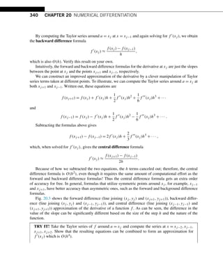
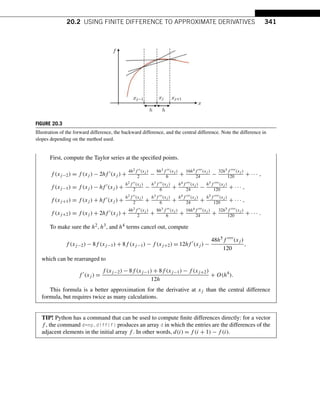
![342 CHAPTER 20 NUMERICAL DIFFERENTIATION
WARNING! When using the command np.diff, the size of the output is one less than the size
of the input since it needs two arguments to produce a difference.
EXAMPLE: Consider the function f (x) = cos(x). We know that the derivative of cos(x) is
−sin(x). Although in practice we may not know the underlying function we are finding the
derivative for, we use the simple example to illustrate the aforementioned numerical differen-
tiation methods and their accuracy. The following code computes the derivatives numerically.
In [1]: import numpy as np
import matplotlib.pyplot as plt
plt.style.use(seaborn-poster)
%matplotlib inline
In [2]: # step size
h = 0.1
# define grid
x = np.arange(0, 2*np.pi, h)
# compute function
y = np.cos(x)
# compute vector of forward differences
forward_diff = np.diff(y)/h
# compute corresponding grid
x_diff = x[:-1:]
# compute exact solution
exact_solution = -np.sin(x_diff)
# Plot solution
plt.figure(figsize = (12, 8))
plt.plot(x_diff, forward_diff, -,
label = Finite difference approximation)
plt.plot(x_diff, exact_solution, label = Exact solution)
plt.legend()
plt.show()
# Compute max error between
# numerical derivative and exact solution
max_error = max(abs(exact_solution - forward_diff))
print(max_error)](https://image.slidesharecdn.com/pythonprogrammingandnumericalmethodsaguideforengineersand-231017183839-0fbc5295/85/Python_Programming_and_Numerical_Methods_A_Guide_for_Engineers_and-pdf-345-320.jpg)
![20.2 USING FINITE DIFFERENCE TO APPROXIMATE DERIVATIVES 343
0.049984407218554114
As the above figure shows, there is a small offset between the two curves, which results from the
numerical error in the evaluation of the numerical derivatives. The maximal error between the two
numerical results is of the order 0.05 and expected to decrease with the size of the step.
As illustrated in the previous example, the finite difference scheme contains a numerical error due
to the approximation of the derivative. This difference decreases with the size of the discretization step,
which is illustrated in the following example.
EXAMPLE: The following code computes the numerical derivative of f (x) = cos(x) using the
forward-difference formula for decreasing step size, h. It then plots the maximum error between
the approximated derivative and the true derivative versus h as shown in the generated figure.
In [3]: # define step size
h = 1
# define number of iterations to perform
iterations = 20
# list to store our step sizes
step_size = []
# list to store max error for each step size
max_error = []
for i in range(iterations):
# halve the step size
h /= 2
# store this step size
step_size.append(h)
# compute new grid
x = np.arange(0, 2 * np.pi, h)](https://image.slidesharecdn.com/pythonprogrammingandnumericalmethodsaguideforengineersand-231017183839-0fbc5295/85/Python_Programming_and_Numerical_Methods_A_Guide_for_Engineers_and-pdf-346-320.jpg)
![344 CHAPTER 20 NUMERICAL DIFFERENTIATION
# compute function value at grid
y = np.cos(x)
# compute vector of forward differences
forward_diff = np.diff(y)/h
# compute corresponding grid
x_diff = x[:-1]
# compute exact solution
exact_solution = -np.sin(x_diff)
# Compute max error between
# numerical derivative and exact solution
max_error.append(max(abs(exact_solution - forward_diff)))
# produce log-log plot of max error versus step size
plt.figure(figsize = (12, 8))
plt.loglog(step_size, max_error, v)
plt.show()
The slope of the line in log–log space is 1; therefore, the error is proportional to h1, which means
that, as expected, the forward-difference formula is O(h).
20.3 APPROXIMATING OF HIGHER ORDER DERIVATIVES
It also possible to use the Taylor series to approximate higher-order derivatives (e.g., f (xj ),f (xj ),
etc.). For example, taking the Taylor series around a = xj and then computing it at x = xj−1 and xj+1
gives
f (xj−1) = f (xj ) − hf
(xj ) +
h2f (xj )
2
−
h3f (xj )
6
+ ···](https://image.slidesharecdn.com/pythonprogrammingandnumericalmethodsaguideforengineersand-231017183839-0fbc5295/85/Python_Programming_and_Numerical_Methods_A_Guide_for_Engineers_and-pdf-347-320.jpg)
![20.4 NUMERICAL DIFFERENTIATION WITH NOISE 345
and
f (xj+1) = f (xj ) + hf
(xj ) +
h2f (xj )
2
+
h3f (xj )
6
+ ··· .
If we add these two equations together, we get
f (xj−1) + f (xj+1) = 2f (xj ) + h2
f
(xj ) +
h4f (xj )
24
+ ··· ,
and, with some rearrangement, this gives the approximation
f
(xj ) ≈
f (xj+1) − 2f (xj ) + f (xj−1)
h2
,
which is O(h2).
20.4 NUMERICAL DIFFERENTIATION WITH NOISE
As stated earlier, sometimes f is given as a vector where f is the corresponding function value for
independent data values in another vector x, which is gridded. Sometimes data can be contaminated
with noise, meaning its value is off by a small amount from what it would be if it were computed from
a pure mathematical function. This can often occur in engineering due to inaccuracies in measurement
devices or the data itself can be slightly modified by perturbations outside the system of interest. For
example, you may be trying to listen to your friend talk in a crowded room. The signal f might be the
intensity and tonal values in your friend’s speech; however, because the room is crowded, noise from
other conversations is heard along with your friend’s speech, and he becomes difficult to understand.
To illustrate this point, we numerically compute the derivative of a simple cosine wave corrupted
by a small sin wave. Consider the following two functions:
f (x) = cos(x)
and
f,ω(x) = cos(x) + sin(ωx)
where 0 1 is a very small number, and ω is a large number. When is small, it is clear that
f f,ω. To illustrate this point, we plot f,ω(x) for = 0.01 and ω = 100, and we can see it is very
close to f (x), as shown in the following figure.
In [1]: import numpy as np
import matplotlib.pyplot as plt
plt.style.use(seaborn-poster)
%matplotlib inline](https://image.slidesharecdn.com/pythonprogrammingandnumericalmethodsaguideforengineersand-231017183839-0fbc5295/85/Python_Programming_and_Numerical_Methods_A_Guide_for_Engineers_and-pdf-348-320.jpg)
![346 CHAPTER 20 NUMERICAL DIFFERENTIATION
In [2]: x = np.arange(0, 2*np.pi, 0.01)
# compute function
omega = 100
epsilon = 0.01
y = np.cos(x)
y_noise = y + epsilon*np.sin(omega*x)
# Plot solution
plt.figure(figsize = (12, 8))
plt.plot(x, y_noise, r-, label = cos(x) + noise)
plt.plot(x, y, b-, label = cos(x))
plt.xlabel(x)
plt.ylabel(y)
plt.legend()
plt.show()
The derivatives of our two test functions are
f
(x) = −sin(x)
and
f
,ω(x) = −sin(x) + ω cos(ωx).
Since ω may not be small when ω is large, the contribution of the noise to the derivative may
not be small. As a result, the derivative (analytic and numerical) may not be usable. For instance, the
following figure shows f (x) and f
,ω(x) for = 0.01 and ω = 100.](https://image.slidesharecdn.com/pythonprogrammingandnumericalmethodsaguideforengineersand-231017183839-0fbc5295/85/Python_Programming_and_Numerical_Methods_A_Guide_for_Engineers_and-pdf-349-320.jpg)
![20.5 SUMMARY AND PROBLEMS 347
In [3]: x = np.arange(0, 2*np.pi, 0.01)
# compute function
y = -np.sin(x)
y_noise = y + epsilon*omega*np.cos(omega*x)
# Plot solution
plt.figure(figsize = (12, 8))
plt.plot(x, y_noise, r-, label = Derivative cos(x) + noise)
plt.plot(x, y, b-, label = Derivative of cos(x))
plt.xlabel(x)
plt.ylabel(y)
plt.legend()
plt.show()
20.5 SUMMARY AND PROBLEMS
20.5.1 SUMMARY
1. Because explicit derivation of functions is sometimes cumbersome for engineering applications,
numerical approaches are preferable.
2. Numerical approximation of derivatives can be done using a grid on which the derivative is approx-
imated by finite differences.
3. Finite differences approximate the derivative by ratios of differences of the function values over
small intervals.
4. Finite difference schemes have different approximation orders depending on the method used.
5. When the data is noisy, there are issues using finite differences for approximating derivatives.](https://image.slidesharecdn.com/pythonprogrammingandnumericalmethodsaguideforengineersand-231017183839-0fbc5295/85/Python_Programming_and_Numerical_Methods_A_Guide_for_Engineers_and-pdf-350-320.jpg)
![348 CHAPTER 20 NUMERICAL DIFFERENTIATION
20.5.2 PROBLEMS
1. Write a function my_der_calc(f, a, b, N, option) with the output as [df,X], where f is a func-
tion object, a and b are scalars such that a b, N is an integer bigger than 10, and option is the
string forward, backward, or central. Let x be an array starting at a, ending at b, contain-
ing N evenly spaced elements, and let y be the array f(x). The output argument, df, should be the
numerical derivatives computed for x and y according to the method defined by the input argument,
option. The output argument X should be an array the same size as df, containing the points in x for
which df is valid. Specifically, the forward difference method “loses” the last point, the backward
difference method loses the first point, and the central difference method loses the first and last
points.
2. Write a function my_num_diff(f,a,b,n,option) with the output as [df,X], where f is a function
object. The function my_num_diff should compute the derivative of f numerically for n evenly
spaced points starting at a and ending at b, according to the method defined by option. The input
argument option is one of the following strings: forward, backward, and central. Note
that for the forward and backward method, the output argument, dy, should be a 1D array of length
n − 1, and for the central difference method dy it should be a 1D array of length n − 2. The function
should also output a vector X that is the same size as dy and denotes the x-values for which dy is
valid.
Test cases:
x = np.linspace(0, 2*np.pi, 100)
f = lambda x: np.sin(x)
[dyf, Xf] = my_num_diff(f, 0, 2*np.pi, 10, forward)
[dyb, Xb] = my_num_diff(f, 0, 2*np.pi, 10, backward)
[dyc, Xc] = my_num_diff(f, 0, 2*np.pi, 10, central)
plt.figure(figsize = (12, 8))
plt.plot(x, np.cos(x), label = analytic)
plt.plot(Xf, dyf, label = forward)
plt.plot(Xb, dyb, label = backward)
plt.plot(Xc, dyc, label = central)
plt.legend()
plt.title(Analytic and Numerical Derivatives of Sine)
plt.xlabel(x)
plt.ylabel(y)
plt.show()](https://image.slidesharecdn.com/pythonprogrammingandnumericalmethodsaguideforengineersand-231017183839-0fbc5295/85/Python_Programming_and_Numerical_Methods_A_Guide_for_Engineers_and-pdf-351-320.jpg)
![20.5 SUMMARY AND PROBLEMS 349
x = np.linspace(0, np.pi, 1000)
f = lambda x: np.sin(np.exp(x))
[dy10, X10] = my_num_diff(f, 0, np.pi, 10, central)
[dy20, X20] = my_num_diff(f, 0, np.pi, 20, central)
[dy100, X100] = my_num_diff(f, 0, np.pi, 100, central)
plt.figure(figsize = (12, 8))
plt.plot(x, np.cos(np.exp(x)), label = analytic)
plt.plot(X10, dy10, label = 10 points)
plt.plot(X20, dy20, label = 20 points)
plt.plot(X100, dy100, label = 100 points)
plt.legend()
plt.title(Analytic and Numerical Derivatives of Sine)
plt.xlabel(x)
plt.ylabel(y)
plt.show()](https://image.slidesharecdn.com/pythonprogrammingandnumericalmethodsaguideforengineersand-231017183839-0fbc5295/85/Python_Programming_and_Numerical_Methods_A_Guide_for_Engineers_and-pdf-352-320.jpg)
![350 CHAPTER 20 NUMERICAL DIFFERENTIATION
3. Write a function my_num_diff_w_smoothing(x,y,n) with output [dy,X], where x and y are a 1D
NumPy array of the same length, and n is a strictly positive scalar. The function should first create
a vector of “smoothed” y data points where y_smooth[i] = np.mean(y[i-n:i+n]). The func-
tion should then compute dy, the derivative of the smoothed y-vector, using the central difference
method. The function should also output a 1D array X that is the same size as dy and denotes the
x-values for which dy is valid.
Assume that the data contained in x is in ascending order with no duplicate entries; it is possible
that the elements of x will not be evenly spaced. Note that the output dy will have 2n + 2 fewer
points than y. Assume that the length of y is much bigger than 2n + 2.
Test cases:
x = np.linspace(0, 2*np.pi, 100)
y = np.sin(x) + np.random.randn(len(x))/100
[dy, X] = my_num_diff_w_smoothing(x, y, 4)
plt.figure(figsize = (12, 12))
plt.subplot(211)
plt.plot(x, y)
plt.title(Noisy Sine function)
plt.xlabel(x)
plt.ylabel(y)
plt.subplot(212)
plt.plot(x, np.cos(x), b, label = cosine)
plt.plot(x[:-1], (y[1:] - y[:-1])/(x[1]-x[0]), g,
label = unsmoothed forward diff)
plt.plot(X, dy, r, label = smoothed)
plt.title(Analytic Derivative and Smoothed Derivative)
plt.xlabel(x)
plt.ylabel(y)
plt.legend()
plt.tight_layout()
plt.show()](https://image.slidesharecdn.com/pythonprogrammingandnumericalmethodsaguideforengineersand-231017183839-0fbc5295/85/Python_Programming_and_Numerical_Methods_A_Guide_for_Engineers_and-pdf-353-320.jpg)
![21
NUMERICAL INTEGRATION
21.1 Numerical Integration Problem Statement ...................................................................... 353
21.2 Riemann Integral .................................................................................................... 354
21.3 Trapezoid Rule....................................................................................................... 356
21.4 Simpson’s Rule ...................................................................................................... 359
21.5 Computing Integrals in Python .................................................................................... 363
21.6 Summary and Problems ............................................................................................ 365
21.6.1 Summary............................................................................................ 365
21.6.2 Problems ............................................................................................ 365
21.1 NUMERICAL INTEGRATION PROBLEM STATEMENT
Given a function f (x), approximate the integral of f (x) over the total interval, [a,b]. Fig. 21.1 illus-
trates this area. To accomplish this goal, we assume that the interval has been discretized into a numeral
grid, x, consisting of n + 1 points with spacing, h = b−a
n . Here, we denote each point in x by xi, where
x0 = a and xn = b. Note that there are n + 1 grid points because the count starts at x0. Assume that the
function, f (x), can be computed for any of the grid points, or that we have been given the function
implicitly as f (xi). The interval [xi,xi+1] is referred to as a subinterval.
FIGURE 21.1
Illustration of the integral. The integral from a to b of the function f is the area below the curve (shaded in grey).
The following sections give some of the most common entry level methods of approximating
b
a f (x)dx. Each method approximates the area under f (x) for each subinterval by a shape for which
it is easy to compute the exact area, and then sums the area contributions of every subinterval.](https://image.slidesharecdn.com/pythonprogrammingandnumericalmethodsaguideforengineersand-231017183839-0fbc5295/85/Python_Programming_and_Numerical_Methods_A_Guide_for_Engineers_and-pdf-355-320.jpg)
![356 CHAPTER 21 NUMERICAL INTEGRATION
TRY IT! Use the left and right Riemann integral, as well as midpoint rule, to approximate
π
0 sin(x)dx with 11 evenly spaced grid points over the whole interval. Compare this value to
the exact value of 2.
In [1]: import numpy as np
a = 0
b = np.pi
n = 11
h = (b - a) / (n - 1)
x = np.linspace(a, b, n)
f = np.sin(x)
I_riemannL = h * sum(f[:n-1])
err_riemannL = 2 - I_riemannL
I_riemannR = h * sum(f[1::])
err_riemannR = 2 - I_riemannR
I_mid = h * sum(np.sin((x[:n-1] + x[1:])/2))
err_mid = 2 - I_mid
print(I_riemannL)
print(err_riemannL)
print(I_riemannR)
print(err_riemannR)
print(I_mid)
print(err_mid)
1.9835235375094546
0.01647646249054535
1.9835235375094546
0.01647646249054535
2.0082484079079745
-0.008248407907974542
21.3 TRAPEZOID RULE
The Trapezoid Rule fits a trapezoid into each subinterval and sums the areas of the trapezoids to
approximate the total integral. This approximation for the integral to an arbitrary function is shown](https://image.slidesharecdn.com/pythonprogrammingandnumericalmethodsaguideforengineersand-231017183839-0fbc5295/85/Python_Programming_and_Numerical_Methods_A_Guide_for_Engineers_and-pdf-358-320.jpg)
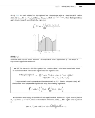
![21.4 SIMPSON’S RULE 359
Since h
2 (f (xi+1) + f (xi)) is the trapezoid rule approximation for the integral over the subinterval,
it is O(h3) for a single subinterval and O(h2) over the whole interval.
TRY IT! Use the trapezoid rule to approximate
π
0 sin(x)dx with 11 evenly spaced grid points
over the whole interval. Compare this value to the exact value of 2.
In [1]: import numpy as np
a = 0
b = np.pi
n = 11
h = (b - a) / (n - 1)
x = np.linspace(a, b, n)
f = np.sin(x)
I_trap = (h/2)*(f[0] + 2 * sum(f[1:n-1]) + f[n-1])
err_trap = 2 - I_trap
print(I_trap)
print(err_trap)
1.9835235375094546
0.01647646249054535
21.4 SIMPSON’S RULE
Consider two consecutive subintervals, [xi−1,xi] and [xi,xi+1]. Simpson’s Rule approximates the
area under f (x) over these two subintervals by fitting a quadratic polynomial through the points
(xi−1,f (xi−1)),(xi,f (xi)), and (xi+1,f (xi+1)), which is a unique polynomial, and then integrates
the quadratic exactly. Fig. 21.3 shows this integral approximation for an arbitrary function.
First, we construct the quadratic polynomial approximation of the function over the two subinter-
vals. The easiest way to do this is to use Lagrange polynomials, which was discussed in Chapter 17.
By applying the formula for constructing Lagrange polynomials, we obtain
Pi(x) = f (xi−1)
(x − xi)(x − xi+1)
(xi−1 − xi)(xi−1 − xi+1)
+ f (xi)
(x − xi−1)(x − xi+1)
(xi − xi−1)(xi − xi+1)
+ f (xi+1)
(x − xi−1)(x − xi)
(xi+1 − xi−1)(xi+1 − xi)
,
and with substitutions for h results in
Pi(x) =
f (xi−1)
2h2
(x − xi)(x − xi+1) −
f (xi)
h2
(x − xi−1)(x − xi+1) +
f (xi+1)
2h2
(x − xi−1)(x − xi).](https://image.slidesharecdn.com/pythonprogrammingandnumericalmethodsaguideforengineersand-231017183839-0fbc5295/85/Python_Programming_and_Numerical_Methods_A_Guide_for_Engineers_and-pdf-361-320.jpg)
![21.4 SIMPSON’S RULE 361
FIGURE 21.4
Illustration of the accounting procedure to approximate the function f by the Simpson rule for the entire interval
[a,b].
and
f (xi+1) = f (xi) + hf
(xi) +
h(xi)
2!
+
h3f (xi)
3!
+
h4f (xi)
4!
+ ··· .
Consider the expression f (xi−1)+4f (xi)+f (xi+1)
6 . Substituting the Taylor series for the respective nu-
merator values produces the equation
f (xi−1) + 4f (xi) + f (xi+1)
6
= f (xi) +
h2
6
f
(xi) +
h4
72
f
(xi) + ··· .
Note that the odd terms cancel out, implying
f (xi) =
f (xi−1) + 4f (xi) + f (xi+1)
6
−
h2
6
f
(xi) + O(h4
).
By substitution of the Taylor series for f (x), the integral of f (x) over two subintervals is then
xi+1
xi−1
f (x)dx =
xi+1
xi−1
f (xi) + f
(xi)(x − xi) +
f (xi)(x − xi)2
2!
+
f (xi)(x − xi)3
3!
+
f (xi)(x − xi)4
4!
+ ···
dx.
Again, we distribute the integral and, without showing it, drop the integrals of terms with odd
powers because they are zero to obtain
xi+1
xi−1
f (x)dx =
xi+1
xi−1
f (xi)dx +
xi+1
xi−1
f (xi)(x − xi)2
2!
dx
+
xi+1
xi−1
f (xi)(x − xi)4
4!
dx + ··· ,](https://image.slidesharecdn.com/pythonprogrammingandnumericalmethodsaguideforengineersand-231017183839-0fbc5295/85/Python_Programming_and_Numerical_Methods_A_Guide_for_Engineers_and-pdf-363-320.jpg)
![362 CHAPTER 21 NUMERICAL INTEGRATION
at which point we perform the integrations. As will soon be clear, computing the integral of the second
term exactly has benefits. The resulting equation is
xi+1
xi−1
f (x)dx = 2hf (xi) +
h3
3
f
(xi) + O(h5
).
Substituting the expression for f (xi) derived earlier, the right-hand side becomes
2h
f (xi−1) + 4f (xi) + f (xi+1)
6
−
h2
6
f
(xi) + O(h4
)
+
h3
3
f
(xi) + O(h5
),
which can be rearranged to
h
3
(f (xi−1) + 4f (xi) + f (xi+1)) −
h3
3
f
(xi) + O(h5
)
+
h3
3
f
(xi) + O(h5
).
Canceling and combining the appropriate terms results in the integral expression
xi+1
xi−1
f (x)dx =
h
3
(f (xi−1) + 4f (xi) + f (xi+1)) + O(h5
).
Recognizing that h
3 (f (xi−1) + 4f (xi) + f (xi+1)) is exactly the Simpson’s rule approximation for
the integral over this subinterval, this equation implies that Simpson’s rule is O(h5) over a subinterval
and O(h4) over the whole interval. Because the h3 terms cancel out exactly, Simpson’s rule gains
another two orders of accuracy!
TRY IT! Use Simpson’s rule to approximate
π
0 sin(x)dx with 11 evenly spaced grid points over
the whole interval. Compare this value to the exact value of 2.
In [1]: import numpy as np
a = 0
b = np.pi
n = 11
h = (b - a) / (n - 1)
x = np.linspace(a, b, n)
f = np.sin(x)
I_simp = (h/3) * (f[0] + 2*sum(f[:n-2:2]) + 4*sum(f[1:n-1:2]) + f[n-1])
err_simp = 2 - I_simp
print(I_simp)
print(err_simp)](https://image.slidesharecdn.com/pythonprogrammingandnumericalmethodsaguideforengineersand-231017183839-0fbc5295/85/Python_Programming_and_Numerical_Methods_A_Guide_for_Engineers_and-pdf-364-320.jpg)
![21.5 COMPUTING INTEGRALS IN PYTHON 363
2.0001095173150043
-0.00010951731500430384
21.5 COMPUTING INTEGRALS IN PYTHON
The scipy.integrate subpackage has several functions for computing integrals. The trapz takes as
input arguments an array of function values f computed on a numerical grid x.
TRY IT! Use the trapz function to approximate
π
0 sin(x)dx for 11 equally spaced points over
the whole interval. Compare this value to the one computed in the earlier example using the
trapezoid rule.
In [1]: import numpy as np
from scipy.integrate import trapz
a = 0
b = np.pi
n = 11
h = (b - a) / (n - 1)
x = np.linspace(a, b, n)
f = np.sin(x)
I_trapz = trapz(f,x)
I_trap = (h/2)*(f[0] + 2 * sum(f[1:n-1]) + f[n-1])
print(I_trapz)
print(I_trap)
1.9835235375094542
1.9835235375094546
Sometimes we need to know the approximated cumulative integral. That is, F(X) =
X
x0
f (x)dx.
For this purpose, it is useful to use the cumtrapz function, which takes the same input arguments as
trapz.
TRY IT! Use the cumtrapz function to approximate the cumulative integral of f (x) = sin(x)
from 0 to π, with a discretization step of 0.01. The exact solution of this integral is F(x) = sin(x).
Plot the results.
In [2]: from scipy.integrate import cumtrapz
import matplotlib.pyplot as plt](https://image.slidesharecdn.com/pythonprogrammingandnumericalmethodsaguideforengineersand-231017183839-0fbc5295/85/Python_Programming_and_Numerical_Methods_A_Guide_for_Engineers_and-pdf-365-320.jpg)
![364 CHAPTER 21 NUMERICAL INTEGRATION
%matplotlib inline
plt.style.use(seaborn-poster)
x = np.arange(0, np.pi, 0.01)
F_exact = -np.cos(x)
F_approx = cumtrapz(np.sin(x), x)
plt.figure(figsize = (10,6))
plt.plot(x, F_exact)
plt.plot(x[1::], F_approx)
plt.grid()
plt.tight_layout()
plt.title($F(x) = int_0^{x} sin(y) dy$)
plt.xlabel(x)
plt.ylabel(f(x))
plt.legend([Exact with Offset, Approx])
plt.show()
The quad(f,a,b) function uses a different numerical differentiation scheme to approximate integrals;
quad integrates the function defined by the function object, f, from a to b.
TRY IT! Use the integrate.quad function to compute
π
0 sin(x)dx. Compare your answer with
the correct answer of 2.
In [3]: from scipy.integrate import quad
I_quad, est_err_quad = quad(np.sin, 0, np.pi)
print(I_quad)](https://image.slidesharecdn.com/pythonprogrammingandnumericalmethodsaguideforengineersand-231017183839-0fbc5295/85/Python_Programming_and_Numerical_Methods_A_Guide_for_Engineers_and-pdf-366-320.jpg)
![366 CHAPTER 21 NUMERICAL INTEGRATION
Test cases:
In: f = lambda x: x**2
my_num_int(f, 0, 1, 3, rect)
Out: 0.625
In: my_num_int(f, 0, 1, 3, trap)
Out: 0.375
In: my_num_int(f, 0, 1, 3, simp)
Out: 0.3333333333333333
In: f = lambda x: np.exp(x**2)
my_num_int(f, -1, 1, 101, simp)
Out: 2.9253035883926493
In: my_num_int(f, -1, 1, 10001, simp)
Out: 2.925303491814364
In: my_num_int(f, -1, 1, 100001, simp)
Out: 2.9253034918143634
5. An earlier chapter demonstrated that some functions can be expressed as an infinite sum of polyno-
mials (i.e., the Taylor series). Other functions, particularly periodic functions, can be written as an
infinite sum of sine and cosine waves. For these functions,
f (x) =
A0
2
+
∞
n=1
An cos(nx) + Bn sin(nx).
It can be shown that the values of An and Bn can be computed using the following formulas:
An =
1
π
π
−π
f (x)cos(nx) dx,
Bn =
1
π
π
−π
f (x)sin(nx) dx.
Just like the Taylor series, functions can be approximated by truncating the Fourier series at some
n = N. Fourier series can be used to approximate some particularly nasty functions, such as the
step function, and they form the basis of many engineering applications, such as signal processing.
Write a function my_fourier_coef(f,n) with output [An,Bn], where f is an function object that
is 2π-periodic. The function my_fourier_coef should compute the nth Fourier coefficients, An and
Bn, in the Fourier series for f defined by the two formulas given earlier. Use the quad function to
perform the integration.](https://image.slidesharecdn.com/pythonprogrammingandnumericalmethodsaguideforengineersand-231017183839-0fbc5295/85/Python_Programming_and_Numerical_Methods_A_Guide_for_Engineers_and-pdf-368-320.jpg)
![21.6 SUMMARY AND PROBLEMS 367
Test cases:
Use the following plotting function to plot the analytic and approximation of functions using the
Fourier series.
def plot_results(f, N):
x = np.linspace(-np.pi, np.pi, 10000)
[A0, B0] = my_fourier_coef(f, 0)
y = A0*np.ones(len(x))/2
for n in range(1, N):
[An, Bn] = my_fourier_coef(f, n)
y += An*np.cos(n*x)+Bn*np.sin(n*x)
plt.figure(figsize = (10,6))
plt.plot(x, f(x), label = analytic)
plt.plot(x, y, label = approximate)
plt.xlabel(x)
plt.ylabel(y)
plt.grid()
plt.legend()
plt.title(f{N}th Order Fourier Approximation)
plt.show()
f = lambda x: np.sin(np.exp(x))
N = 2
plot_results(f, N)
N = 2
plot_results(f, N)](https://image.slidesharecdn.com/pythonprogrammingandnumericalmethodsaguideforengineersand-231017183839-0fbc5295/85/Python_Programming_and_Numerical_Methods_A_Guide_for_Engineers_and-pdf-369-320.jpg)
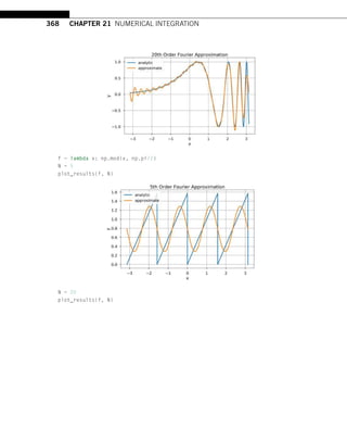
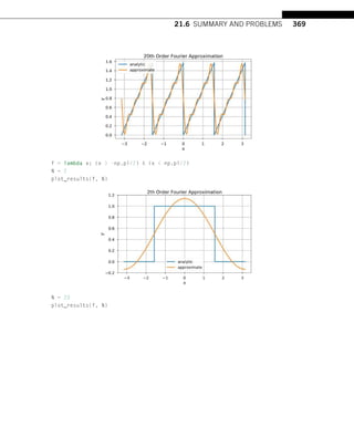
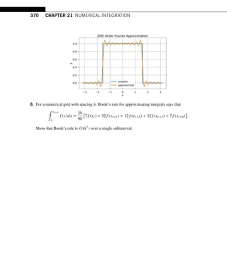
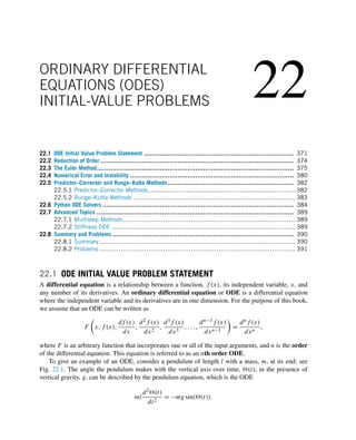
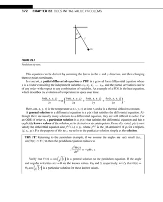
![376 CHAPTER 22 ODES INITIAL-VALUE PROBLEMS
interval [t0,tf ] with spacing h. Without loss of generality, we assume that t0 = 0 and that tf = Nh for
some positive integer, N.
The linear approximation of S(t) around tj at tj+1 is
S(tj+1) = S(tj ) + (tj+1 − tj )
dS(tj )
dt
,
which can also be written
S(tj+1) = S(tj ) + hF(tj ,S(tj )).
This formula is called the Explicit Euler Formula. It allows us to compute an approximation for
the state at S(tj+1) given the state at S(tj ). This is actually based on the Taylor series we discussed in
Chapter 18, whereby we used only the first order item in Taylor series to linearly approximate the next
solution. Later in this chapter, we will present a formula using higher terms to increase the accuracy.
Starting from a given initial value of S0 = S(t0), we can use this formula to integrate the states up to
S(tf ); these S(t) values are then an approximation for the solution of the differential equation. The
explicit Euler formula is the simplest and most intuitive method for solving initial value problems. At
any state (tj ,S(tj )) it uses F at that state to “point” linearly toward the next state and then moves in
that direction a distance of h, as shown in Fig. 22.2.
FIGURE 22.2
The illustration of the explicit Euler method.
Although there are more sophisticated and accurate methods for solving these problems, they all
have the same fundamental structure. As such, we enumerate explicitly the steps for solving an initial
value problem using the explicit Euler formula.
WHAT IS HAPPENING? Assume we are given a function F(t,S(t)) that computes dS(t)
dt , a
numerical grid, t, of the interval, [t0,tf ], and an initial state value S0 = S(t0). We can compute
S(tj ) for every tj in t using the following steps:](https://image.slidesharecdn.com/pythonprogrammingandnumericalmethodsaguideforengineersand-231017183839-0fbc5295/85/Python_Programming_and_Numerical_Methods_A_Guide_for_Engineers_and-pdf-378-320.jpg)
![22.3 THE EULER METHOD 377
1. Store S0 = S(t0) in an array, S.
2. Compute S(t1) = S0 + hF(t0,S0).
3. Store S1 = S(t1) in S.
4. Compute S(t2) = S1 + hF(t1,S1).
5. Store S2 = S(t1) in S.
6. ...
7. Compute S(tf ) = Sf −1 + hF(tf −1,Sf −1).
8. Store Sf = S(tf ) in S.
9. S is an approximation of the solution to the initial value problem.
When using a method with this structure, we say the method integrates the solution of the ODE.
TRY IT! The differential equation df (t)
dt = e−t with initial condition f0 = −1 has the exact solu-
tion f (t) = −e−t . Approximate the solution to this initial value problem between zero and 1 in
increments of 0.1 using the explicit Euler formula. Plot the difference between the approximated
solution and the exact solution.
In [1]: import numpy as np
import matplotlib.pyplot as plt
plt.style.use(seaborn-poster)
%matplotlib inline
# Define parameters
f = lambda t, s: np.exp(-t) # ODE
h = 0.1 # Step size
t = np.arange(0, 1 + h, h) # Numerical grid
s0 = -1 # Initial Condition
# Explicit Euler Method
s = np.zeros(len(t))
s[0] = s0
for i in range(0, len(t) - 1):
s[i + 1] = s[i] + h*f(t[i], s[i])
plt.figure(figsize = (12, 8))
plt.plot(t, s, b-, label=Approximate)
plt.plot(t, -np.exp(-t), g, label=Exact)
plt.title(Approximate and Exact Solution for Simple ODE)
plt.xlabel(t)
plt.ylabel(f(t))](https://image.slidesharecdn.com/pythonprogrammingandnumericalmethodsaguideforengineersand-231017183839-0fbc5295/85/Python_Programming_and_Numerical_Methods_A_Guide_for_Engineers_and-pdf-379-320.jpg)
![378 CHAPTER 22 ODES INITIAL-VALUE PROBLEMS
plt.grid()
plt.legend(loc=lower right)
plt.show()
In the above figure, each dot is one approximation based on the previous dot in a linear fashion.
From the initial value, we can eventually obtain an approximation of the solution on the numerical grid.
If we repeat the process for h = 0.01, we obtain a better approximation for the solution:
In [2]: h = 0.01 # Step size
t = np.arange(0, 1 + h, h) # Numerical grid
s0 = -1 # Initial Condition
# Explicit Euler Method
s = np.zeros(len(t))
s[0] = s0
for i in range(0, len(t) - 1):
s[i + 1] = s[i] + h*f(t[i], s[i])
plt.figure(figsize = (12, 8))
plt.plot(t, s, b-, label=Approximate)
plt.plot(t, -np.exp(-t), g, label=Exact)
plt.title(Approximate and Exact Solution for Simple ODE)
plt.xlabel(t)
plt.ylabel(f(t))
plt.grid()
plt.legend(loc=lower right)
plt.show()](https://image.slidesharecdn.com/pythonprogrammingandnumericalmethodsaguideforengineersand-231017183839-0fbc5295/85/Python_Programming_and_Numerical_Methods_A_Guide_for_Engineers_and-pdf-380-320.jpg)
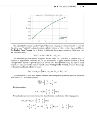
![380 CHAPTER 22 ODES INITIAL-VALUE PROBLEMS
Similarly, we can plug the same expression into the implicit Euler formula to obtain
1 −h
gh
l 1
S(tj+1) = S(tj ),
and into the trapezoidal formula to obtain
1 −h
2
gh
2l 1
S(tj+1) =
1 h
2
−gh
2l 1
S(tj ).
With some rearrangement, these equations become respectively
S(tj+1) =
1 −h
gh
l 1
−1
S(tj ),
S(tj+1) =
1 −h
2
gh
2l 1
−1
1 h
2
−gh
2l 1
S(tj ).
These equations allow us to solve the initial value problem since at each state, S(tj ), we can com-
pute the next state at S(tj+1). In general, this is possible to do when an ODE is linear.
22.4 NUMERICAL ERROR AND INSTABILITY
There are two main issues to consider with regard to integration schemes for ODEs: accuracy and
stability. Accuracy refers to a scheme’s ability to get close to the exact solution, which is usually
unknown, as a function of the step size h. Previous chapters have referred to accuracy using the notation
O(hp). The same notation can be used to solve ODEs. The stability of an integration scheme is its
ability to keep the error from growing as it integrates forward in time. If the error does not grow, then
the scheme is stable; otherwise it is unstable. Some integration schemes are stable for certain choices
of h and unstable for others; these integration schemes are also referred to as unstable.
To illustrate issues of stability, we numerically solve the pendulum equation using the explicit and
implicit Euler, as well as trapezoidal, formulas.
TRY IT! Use the explicit and implicit Euler, as well as trapezoidal, formulas to solve the pen-
dulum equation over the time interval [0,5] in increments of 0.1, and for an initial solution of
S0 =
1
0
. For the model parameters using
g
l = 4, plot the approximate solution on a single
graph.
In [1]: import numpy as np
from numpy.linalg import inv](https://image.slidesharecdn.com/pythonprogrammingandnumericalmethodsaguideforengineersand-231017183839-0fbc5295/85/Python_Programming_and_Numerical_Methods_A_Guide_for_Engineers_and-pdf-382-320.jpg)
![22.4 NUMERICAL ERROR AND INSTABILITY 381
import matplotlib.pyplot as plt
plt.style.use(seaborn-poster)
%matplotlib inline
In [2]: # define step size
h = 0.1
# define numerical grid
t = np.arange(0, 5.1, h)
# oscillation freq. of pendulum
w = 4
s0 = np.array([[1], [0]])
m_e = np.array([[1, h],
[-w**2*h, 1]])
m_i = inv(np.array([[1, -h],
[w**2*h, 1]]))
m_t = np.dot(inv(np.array([[1, -h/2],
[w**2*h/2,1]])), np.array(
[[1,h/2], [-w**2*h/2, 1]]))
s_e = np.zeros((len(t), 2))
s_i = np.zeros((len(t), 2))
s_t = np.zeros((len(t), 2))
# do integrations
s_e[0, :] = s0.T
s_i[0, :] = s0.T
s_t[0, :] = s0.T
for j in range(0, len(t)-1):
s_e[j+1, :] = np.dot(m_e,s_e[j, :])
s_i[j+1, :] = np.dot(m_i,s_i[j, :])
s_t[j+1, :] = np.dot(m_t,s_t[j, :])
plt.figure(figsize = (12, 8))
plt.plot(t,s_e[:,0],b-)
plt.plot(t,s_i[:,0],g:)
plt.plot(t,s_t[:,0],r-)
plt.plot(t, np.cos(w*t), k)
plt.ylim([-3, 3])
plt.xlabel(t)](https://image.slidesharecdn.com/pythonprogrammingandnumericalmethodsaguideforengineersand-231017183839-0fbc5295/85/Python_Programming_and_Numerical_Methods_A_Guide_for_Engineers_and-pdf-383-320.jpg)
![382 CHAPTER 22 ODES INITIAL-VALUE PROBLEMS
plt.ylabel($Theta (t)$)
plt.legend([Explicit, Implicit, Trapezoidal, Exact])
plt.show()
The generated figure above compares the numerical solution to the pendulum problem. The exact
solution is a pure cosine wave. The explicit Euler scheme is clearly unstable. The implicit Euler scheme
decays exponentially, which is not correct. The trapezoidal method captures the solution correctly, with
a small phase shift as time increases.
22.5 PREDICTOR–CORRECTOR AND RUNGE–KUTTA METHODS
22.5.1 PREDICTOR–CORRECTOR METHODS
Given any time and state value, the function, F(t,S(t)), returns the change of state dS(t)
dt . The
predictor–corrector methods of solving initial value problems improve the approximation accuracy of
non-predictor–corrector methods by querying the F function several times at different locations (pre-
dictions). Then, using a weighted average of the results (corrections), updates the state. Essentially, it
uses two formulas: a predictor and a corrector. The predictor is an explicit formula and estimates
the solution at tj+1 first, i.e., we can use Euler method or some other methods to finish this step. Af-
ter obtaining the solution S(tj+1), we apply the corrector to improve the accuracy. Using the found
S(tj+1) on the right-hand side of an otherwise implicit formula, the corrector can calculate a new,
more accurate solution.
The midpoint method has a predictor step:
S
tj +
h
2
= S(tj ) +
h
2
F(tj ,S(tj )),
which is the prediction of the solution value halfway between tj and tj+1.](https://image.slidesharecdn.com/pythonprogrammingandnumericalmethodsaguideforengineersand-231017183839-0fbc5295/85/Python_Programming_and_Numerical_Methods_A_Guide_for_Engineers_and-pdf-384-320.jpg)
![22.5 PREDICTOR–CORRECTOR AND RUNGE–KUTTA METHODS 383
It then computes the corrector step:
S(tj+1) = S(tj ) + hF
tj +
h
2
,S
tj +
h
2
,
which computes the solution at S(tj+1) from S(tj ) but uses the derivative from S
tj + h
2
.
22.5.2 RUNGE–KUTTA METHODS
Runge–Kutta (RK) methods are among the most widely used methods for solving ODEs. Recall that
the Euler method uses the first two terms in Taylor series to approximate the numerical integration,
which is linear: S(tj+1) = S(tj + h) = S(tj ) + h · S(tj ).
We can greatly improve the accuracy of numerical integration if we keep more terms of the series
as
S(tj+1) = S(tj + h) = S(tj ) + S
(tj )h +
1
2!
S
(tj )h2
+ ··· +
1
n!
S(n)
(tj )hn
.
In order to obtain this more accurate solution, we need to derive the expressions of S(tj ),S(tj ),
...,S(n)(tj ). This extra work can be avoided using the RK methods, which are based on truncated
Taylor series but do not require computation of these higher derivatives.
22.5.2.1 Second-Order Runge–Kutta Method
Let us first derive the second order RK method. Let dS(t)
dt = F(t,S(t)). Then we assume an integration
formula the form of
S(t + h) = S(t) + c1F(t,S(t))h + c2F[t + ph,S(t) + qhF(t,S(t))]h. (22.1)
We can attempt to find these parameters c1,c2,p,q by matching the above equation to the second-
order Taylor series:
S(t + h) = S(t) + S
(t)h +
1
2!
S
(t)h2
= S(t) + F(t,S(t))h +
1
2!
F
(t,S(t))h2
. (22.2)
Note that
F
(t,s(t)) =
∂F
∂t
+
∂F
∂S
∂S
∂t
=
∂F
∂t
+
∂F
∂S
F. (22.3)
Therefore, Eq. (22.2) can be written as
S(t + h) = S + Fh +
1
2!
∂F
∂t
+
∂F
∂S
F
h2
. (22.4)
In Eq. (22.1), we rewrite the last term by applying Taylor series in several variables:
F[t + ph,S + qhF)] = F +
∂F
∂t
ph + qh
∂F
∂S
F,](https://image.slidesharecdn.com/pythonprogrammingandnumericalmethodsaguideforengineersand-231017183839-0fbc5295/85/Python_Programming_and_Numerical_Methods_A_Guide_for_Engineers_and-pdf-385-320.jpg)
![22.6 PYTHON ODE SOLVERS 385
CONSTRUCTION:
Let F be a function object to the function that computes
dS(t)
dt
= F(t,S(t)),
S(t0) = S0.
The variable t is a one-dimensional independent variable (time), S(t) is an n-dimensional
vector-valued function (state), and F(t,S(t)) defines the differential equations; S0 is an initial
value for S. The function F must have the form dS = F(t,S), although the name does not have
to be F. The goal is to find the S(t) that approximately satisfies the differential equations given
the initial value S(t0) = S0.
Using the solver to solve the differential equation is as follows:
solve_ivp(fun,t_span,s0,method RK45,t_eval=None)
where fun takes in the function in the right-hand side of the system; t_span is the interval of
integration (t0,tf ) where t0 is the start and tf is the end of the interval; s0 is the initial state. There
are a couple of methods to choose from: the default is “RK45”, which is the explicit Runge–Kutta
method of order 5(4). There are other methods you can use as well; see the end of this section for
more information; t_eval takes in the times at which to store the computed solution, and must be
sorted and lie within t_span.
Let us try one example below.
EXAMPLE: Consider the ODE
dS(t)
dt
= cos(t)
for an initial value of S0 = 0. The exact solution to this problem is S(t) = sin(t). Use solve_ivp to
approximate the solution to this initial value problem over the interval [0,π]. Plot the approximate
solution versus the exact solution and the relative error over time.
In [1]: import matplotlib.pyplot as plt
import numpy as np
from scipy.integrate import solve_ivp
plt.style.use(seaborn-poster)
%matplotlib inline
F = lambda t, s: np.cos(t)](https://image.slidesharecdn.com/pythonprogrammingandnumericalmethodsaguideforengineersand-231017183839-0fbc5295/85/Python_Programming_and_Numerical_Methods_A_Guide_for_Engineers_and-pdf-387-320.jpg)
![386 CHAPTER 22 ODES INITIAL-VALUE PROBLEMS
t_eval = np.arange(0, np.pi, 0.1)
sol = solve_ivp(F, [0, np.pi], [0], t_eval=t_eval)
plt.figure(figsize = (12, 4))
plt.subplot(121)
plt.plot(sol.t, sol.y[0])
plt.xlabel(t)
plt.ylabel(S(t))
plt.subplot(122)
plt.plot(sol.t, sol.y[0] - np.sin(sol.t))
plt.xlabel(t)
plt.ylabel(S(t) - sin(t))
plt.tight_layout()
plt.show()
The above left figure shows the integration of dS(t)
dt = cos(t) with solve_ivp. The right figure com-
putes the difference between the solution of the integration by solve_ivp and evaluates the analytical
solution to this ODE. As can be seen from the figure, the difference between the approximate and exact
solution to this ODE is small. Also, we can control the relative and absolute tolerances using the rtol
and atol arguments; the solver keeps the local error estimates less than atol + rtol*abs(S). The
default values are 1e-3 for rtol and 1e-6 for atol.
TRY IT! Using the rtol and atol to make the difference between the approximate and exact
solution less than 1e-7.
In [2]: sol = solve_ivp(F, [0, np.pi], [0], t_eval=t_eval,
rtol = 1e-8, atol = 1e-8)
plt.figure(figsize = (12, 4))
plt.subplot(121)
plt.plot(sol.t, sol.y[0])
plt.xlabel(t)
plt.ylabel(S(t))
plt.subplot(122)
plt.plot(sol.t, sol.y[0] - np.sin(sol.t))](https://image.slidesharecdn.com/pythonprogrammingandnumericalmethodsaguideforengineersand-231017183839-0fbc5295/85/Python_Programming_and_Numerical_Methods_A_Guide_for_Engineers_and-pdf-388-320.jpg)
![22.6 PYTHON ODE SOLVERS 387
plt.xlabel(t)
plt.ylabel(S(t) - sin(t))
plt.tight_layout()
plt.show()
EXAMPLE: Consider the ODE
dS(t)
dt
= −S(t),
with an initial value of S0 = 1. The exact solution to this problem is S(t) = e−t . Use solve_ivp to
approximate the solution to this initial value problem over the interval [0,1]. Plot the approximate
solution versus the exact solution, and the relative error over time.
In [3]: F = lambda t, s: -s
t_eval = np.arange(0, 1.01, 0.01)
sol = solve_ivp(F, [0, 1], [1], t_eval=t_eval)
plt.figure(figsize = (12, 4))
plt.subplot(121)
plt.plot(sol.t, sol.y[0])
plt.xlabel(t)
plt.ylabel(S(t))
plt.subplot(122)
plt.plot(sol.t, sol.y[0] - np.exp(-sol.t))
plt.xlabel(t)
plt.ylabel(S(t) - exp(-t))
plt.tight_layout()
plt.show()](https://image.slidesharecdn.com/pythonprogrammingandnumericalmethodsaguideforengineersand-231017183839-0fbc5295/85/Python_Programming_and_Numerical_Methods_A_Guide_for_Engineers_and-pdf-389-320.jpg)
![388 CHAPTER 22 ODES INITIAL-VALUE PROBLEMS
The above figure shows the corresponding numerical results. As in the previous example, the dif-
ference between the result of solve_ivp and the evaluation of the analytical solution by Python is very
small compared to the value of the function.
EXAMPLE: Let the state of a system be defined by S(t) =
x(t)
y(t)
, and let the evolution of the
system be defined by the ODE
dS(t)
dt
=
0 t2
−t 0
S(t).
Use solve_ivp to solve this ODE for the time interval [0,10] with an initial value of S0 =
1
1
. Plot the solution in (x(t),y(t)).
In [4]: F=lambda t, s: np.dot(np.array([[0, t**2], [-t,0]]),s)
t_eval = np.arange(0, 10.01, 0.01)
sol = solve_ivp(F, [0, 10], [1, 1], t_eval=t_eval)
plt.figure(figsize = (12, 8))
plt.plot(sol.y.T[:, 0], sol.y.T[:, 1])
plt.xlabel(x)
plt.ylabel(y)
plt.show()](https://image.slidesharecdn.com/pythonprogrammingandnumericalmethodsaguideforengineersand-231017183839-0fbc5295/85/Python_Programming_and_Numerical_Methods_A_Guide_for_Engineers_and-pdf-390-320.jpg)
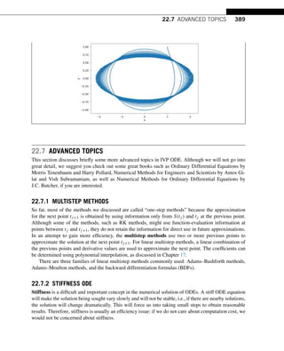
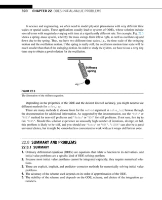
![22.8 SUMMARY AND PROBLEMS 391
22.8.2 PROBLEMS
1. The logistic equation is a simple differential equation model that can be used to relate the change
in population dP
dt to the current population, P, given a growth rate, r, and a carrying capacity, K.
The logistic equation can be expressed by
dP
dt
= rP
1 −
P
K
.
Write a function my_logistic_eq(t, P, r, K) that represents the logistic equation with a return
of dP. Note that this format allows my_logistic_eq to be used as an input argument to solve_ivp.
Assume that the arguments dP, t, P, r, and K are all scalars, and dP is the value dP
dt given r, P,
and K. Note that the input argument, t, is obligatory if my_logistic_eq is to be used as an input
argument to solve_ivp, even though it is part of the differential equation.
Note that the logistic equation has an analytic solution defined by
P(t) =
KP0ert
K + P0(ert − 1)
where P0 is the initial population. Verify that this equation is a solution to the logistic equation.
Test cases:
In [1]: import numpy as np
from scipy.integrate import solve_ivp
import matplotlib.pyplot as plt
from functools import partial
plt.style.use(seaborn-poster)
%matplotlib inline
In [2]: def my_logistic_eq(t, P, r, K):
# put your code here
return dP
dP = my_logistic_eq(0, 10, 1.1, 15)
dP
Out[2]: 3.666666666666667
In [3]: from functools import partial
t0 = 0
tf = 20
P0 = 10
r = 1.1
K = 20
t = np.linspace(0, 20, 2001)](https://image.slidesharecdn.com/pythonprogrammingandnumericalmethodsaguideforengineersand-231017183839-0fbc5295/85/Python_Programming_and_Numerical_Methods_A_Guide_for_Engineers_and-pdf-393-320.jpg)
![392 CHAPTER 22 ODES INITIAL-VALUE PROBLEMS
f = partial(my_logistic_eq, r=r, K=K)
sol=solve_ivp(f,[t0,tf],[P0],t_eval=t)
plt.figure(figsize = (10, 8))
plt.plot(sol.t, sol.y[0])
plt.plot(t, K*P0*np.exp(r*t)/(K+P0*(np.exp(r*t)-1)),r:)
plt.xlabel(time)
plt.ylabel(population)
plt.legend([Numerical Solution, Exact Solution])
plt.grid(True)
plt.show()
2. The Lorenz attractor is a system of ordinary differential equations that was originally developed
to model convection currents in the atmosphere. The Lorenz equations can be written as fol-
lows:
dx
dt
= σ(y − x),
dy
dt
= x(ρ − z) − y,
dz
dt
= xy − βz,](https://image.slidesharecdn.com/pythonprogrammingandnumericalmethodsaguideforengineersand-231017183839-0fbc5295/85/Python_Programming_and_Numerical_Methods_A_Guide_for_Engineers_and-pdf-394-320.jpg)
![22.8 SUMMARY AND PROBLEMS 393
where x, y, and z represent the position in three dimensions, and σ,ρ, and β are scalar parameters
of the system. Read more about the Lorenz attractor on Wikipedia1 or more details in the book
“Viability Theory – New Directions.” Write a function my_lorenz(t,S,sigma,rho,beta) where t
is a scalar denoting time, S is a 3D array denoting the position (x,y,z), and sigma, rho, and beta
are strictly positive scalars representing σ,ρ, and β. The output argument dS should be the same
size as S.
Test cases:
In [4]: def my_lorenz(t, S, sigma, rho, beta):
# put your code here
return dS
s = np.array([1, 2, 3])
dS = my_lorenz(0, s, 10, 28, 8/3)
dS
Out[4]: array([10., 23., -6.])
3. Write a function my_lorenz_solver(t_span,s0,sigma,rho,beta) solves the Lorenz equations us-
ing solve_ivp, the function returns [T,X,Y,Z]. The input argument t_span should be a list of the
form [t0,tf ], where t0 is the initial time, and tf is the final time of consideration. The input ar-
gument s0 should be a 3D array of the form [x0,y0,z0], where (x0,y0,z0) represents an initial
position. Finally, the input arguments sigma, rho, and β are the scalar parameters σ,ρ, and β of
the Lorenz system. The output argument T should be an array of times given as the output argu-
ment of solve_ivp. The output arguments, X, Y, and Z should be the numerically integrated solution
produced from my_lorenz in the previous problem and solve_ivp.
Test cases:
In [5]: def my_lorenz_solver(t_span, s0, sigma, rho, beta):
# put your code here
return [T, X, Y, Z]
sigma = 10
rho = 28
beta = 8/3
t0 = 0
tf = 50
s0 = np.array([0, 1, 1.05])
[T, X, Y, Z] = my_lorenz_solver([t0, tf], s0, sigma, rho, beta)
1 https://en.wikipedia.org/wiki/Lorenz_system.](https://image.slidesharecdn.com/pythonprogrammingandnumericalmethodsaguideforengineersand-231017183839-0fbc5295/85/Python_Programming_and_Numerical_Methods_A_Guide_for_Engineers_and-pdf-395-320.jpg)
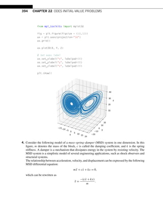
![22.8 SUMMARY AND PROBLEMS 395
Let the state of the system be denoted by the vector S = [x;v] where x is the displacement of the
mass from its resting configuration, and v is its velocity. Rewrite the MSD equation as a first-order
differential equation in terms of the state, S. In other words, rewrite the MSD equation as dS/dt =
f (t,S).
Write a function my_msd(t,S,m,c,k) where t is a scalar denoting time, S is a 2D vector denoting
the state of the MSD system, and m, c, and k are the mass, damping, and stiffness coefficients of the
MSD equation, respectively.
Test cases:
In [6]: def my_msd(t, S, m, c, k):
# put your code here
return ds
my_msd(0, [1, -1], 10, 1, 100)
Out[6]: array([-1. , -9.9])
In [7]: m = 1
k = 10
f = partial(my_msd, m=m, c=0, k=k)
t_e = np.arange(0, 20, 0.1)
sol_1=solve_ivp(f,[0,20],[1,0],t_eval=t_e)
f = partial(my_msd, m=m, c=1, k=k)
sol_2=solve_ivp(f,[0,20],[1,0],t_eval=t_e)
f = partial(my_msd, m=m, c=10, k=k)
sol_3=solve_ivp(f,[0,20],[1,0],t_eval=t_e)
plt.figure(figsize = (10, 8))
plt.plot(sol_1.t, sol_1.y[0])
plt.plot(sol_2.t, sol_2.y[0])
plt.plot(sol_3.t, sol_3.y[0])
plt.title(Numerical Solution of MSD System with Varying Dampling)
plt.xlabel(time)
plt.ylabel(displacement)
plt.legend([no dampling, c=1, critically damped], loc=1)](https://image.slidesharecdn.com/pythonprogrammingandnumericalmethodsaguideforengineersand-231017183839-0fbc5295/85/Python_Programming_and_Numerical_Methods_A_Guide_for_Engineers_and-pdf-397-320.jpg)
![396 CHAPTER 22 ODES INITIAL-VALUE PROBLEMS
5. Write a function my_forward_euler(ds,t_span,s0) where ds is a function object, f (t,s), describ-
ing a first-order differential equation, t_span is an array of times for which numerical solutions of
the differential equation are desired, and s0 is the initial condition of the system. Assume that the
size of the state is one. The output argument should be a list of [t,s], such that t[i] = t_span[i]
for all i, and s should be the integrated values of ds at times t. Perform the integration using the
forward Euler method, s[ti] = s[ti−1] + (ti − ti−1)ds(ti−1,s[ti−1]). Note that s[0] should equal s0.
Test cases:
In [8]: def my_forward_euler(ds, t_span, s0):
# put your code here
return [t, s]
t_span = np.linspace(0, 1, 10)
s0 = 1
# Define parameters
f = lambda t, s: t*np.exp(-s)
t_eul, s_eul = my_forward_euler(f, t_span, s0)
print(t_eul)
print(s_eul)
[0. 0.11111111 0.22222222 0.33333333 0.44444444 0.55555556
0.66666667 0.77777778 0.88888889 1. ]
[1. 1. 1.00454172 1.013584 1.02702534 1.04470783
1.06642355 1.09192262 1.12092255 1.153118 ]](https://image.slidesharecdn.com/pythonprogrammingandnumericalmethodsaguideforengineersand-231017183839-0fbc5295/85/Python_Programming_and_Numerical_Methods_A_Guide_for_Engineers_and-pdf-398-320.jpg)
![22.8 SUMMARY AND PROBLEMS 397
In [9]: plt.figure(figsize = (10, 8))
# Exact solution
t = np.linspace(0, 1, 1000)
s = np.log(np.exp(s0) + (t**2-t[0])/2)
plt.plot(t, s, r, label=Exact)
# Forward Euler
plt.plot(t_eul, s_eul, g, label=Euler)
# Python solver
sol = solve_ivp(f, [0, 1], [s0], t_eval=t)
plt.plot(sol.t, sol.y[0], b-, label=Python Solver)
plt.xlabel(t)
plt.ylabel(f(t))
plt.grid()
plt.legend(loc=2)
plt.show()
6. Write a function myRK4(ds,t_span,s0), where the input and output arguments are the same as in
Problem 5. The function myRK4 should numerically integrate ds using the fourth-order Runge–Kutta
method.
Test cases:
In [10]: def myRK4(ds, t_span, s0):
# put your code here
return [t, s]](https://image.slidesharecdn.com/pythonprogrammingandnumericalmethodsaguideforengineersand-231017183839-0fbc5295/85/Python_Programming_and_Numerical_Methods_A_Guide_for_Engineers_and-pdf-399-320.jpg)
![398 CHAPTER 22 ODES INITIAL-VALUE PROBLEMS
f = lambda t, s: np.sin(np.exp(s))/(t+1)
t_span = np.linspace(0, 2*np.pi, 10)
s0 = 0
plt.figure(figsize = (10, 8))
# Runge-Kutta method
t, s = myRK4(f, t_span, s0)
plt.plot(t, s, r, label=RK4)
# Python solver
sol = solve_ivp(f, [0, 2*np.pi], [s0], t_eval=t)
plt.plot(sol.t, sol.y[0], b-, label=Python Solver)
plt.xlabel(t)
plt.ylabel(f(t))
plt.grid()
plt.legend(loc=2)
plt.show()](https://image.slidesharecdn.com/pythonprogrammingandnumericalmethodsaguideforengineersand-231017183839-0fbc5295/85/Python_Programming_and_Numerical_Methods_A_Guide_for_Engineers_and-pdf-400-320.jpg)
![23
BOUNDARY-VALUE PROBLEMS
FOR ORDINARY DIFFERENTIAL
EQUATIONS (ODES)
23.1 ODE Boundary Value Problem Statement ........................................................................ 399
23.2 The Shooting Method ............................................................................................... 401
23.3 The Finite Difference Method...................................................................................... 406
23.4 Numerical Error and Instability ................................................................................... 411
23.5 Summary and Problems ............................................................................................ 412
23.5.1 Summary............................................................................................ 412
23.5.2 Problems ............................................................................................ 412
23.1 ODE BOUNDARY VALUE PROBLEM STATEMENT
The previous chapter introduced ordinary differential equation initial-value problems. For initial value
problems, all the known values are specified at the same value of the independent variable, usually at
the lower boundary of the interval; this is where the term “initial” comes from. This chapter introduces
another type of problem, namely the boundary-value problem. As the name suggests, the known
values are specified at the extremes of the independent variable, i.e., the boundaries of the interval.
For example, if we have a simple second-order ordinary differential equation,
d2f (x)
dx2
=
df (x)
dx
+ 3
and if the independent variable varies over the domain of [0,20], the initial value problem will have
the two conditions at the value of zero: that is, we know the value of f (0) and f (0). In contrast,
boundary-value problems will specify the values at x = 0 and x = 20. Note that to solve a first-order
ODE to obtain a particular solution requires one constraint, while an nth-order ODE requires n con-
straints.
The boundary-value problem for an nth-order ordinary differential equation,
F
x,f (x),
df (x)
dx
,
d2f (x)
dx2
,
d3f (x)
dx3
,...,
dn−1f (x)
dxn−1
=
dnf (x)
dxn
,
specifies n known boundary conditions at a and b, to solve this equation on an interval of x ∈ [a,b].
For the second-order case, since the boundary condition can be either be a value of f (x) or a value of
the derivative f (x), we can have several different cases for the specified values. For example, we can
have the boundary condition values specified as:](https://image.slidesharecdn.com/pythonprogrammingandnumericalmethodsaguideforengineersand-231017183839-0fbc5295/85/Python_Programming_and_Numerical_Methods_A_Guide_for_Engineers_and-pdf-401-320.jpg)
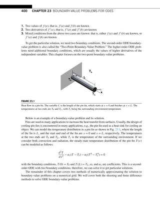
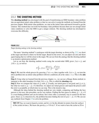
![402 CHAPTER 23 BOUNDARY-VALUE PROBLEMS FOR ODES
off the ground after 5 s after launch, what should be the velocity at launch? (Assuming we ignore
the drag of the air resistance.)
To answer this question, we can frame the problem as a boundary-value problem for a second-
order ODE. The ODE is
d2y
dt2
= −g,
and the two boundary conditions are y(0) = 0 and y(5) = 50. We want to answer the question:
What’s y(0) at launch?
This is a quite simple question and can be solved analytically quite easily; the correct answer
y(0) = 34.5. If we solve it using the shooting method, we need to reduce the order of the function
first, and the second-order ODE becomes:
dy
dt
= v,
dv
dt
= −g.
Therefore, we have S(t) =
y(t)
v(t)
which satisfies
dS(t)
dt
=
0 1
0 −g/v
S(t).
In [1]: import numpy as np
import matplotlib.pyplot as plt
from scipy.integrate import solve_ivp
plt.style.use(seaborn-poster)
%matplotlib inline
For our first guess, we take the velocity at launch as 25 m/s.
In [2]: F = lambda t, s: np.dot(np.array([[0,1],[0,-9.8/s[1]]]),s)
t_span = np.linspace(0, 5, 100)
y0 = 0
v0 = 25
t_eval = np.linspace(0, 5, 10)
sol = solve_ivp(F, [0, 5], [y0, v0], t_eval = t_eval)
plt.figure(figsize = (10, 8))
plt.plot(sol.t, sol.y[0])
plt.plot(5, 50, ro)
plt.xlabel(time (s))](https://image.slidesharecdn.com/pythonprogrammingandnumericalmethodsaguideforengineersand-231017183839-0fbc5295/85/Python_Programming_and_Numerical_Methods_A_Guide_for_Engineers_and-pdf-404-320.jpg)
![23.2 THE SHOOTING METHOD 403
plt.ylabel(altitude (m))
plt.title(ffirst guess v={v0} m/s)
plt.show()
The figure shows that the first guess is a little too small, since after 5 s for the chosen initial
velocity, the altitude of the rocket is less than 10 m. The red dot in the figure is the target we want
to hit. If we adjust our guess and increase the velocity to 40 m/s, then we obtain:
In [3]: v0 = 40
sol = solve_ivp(F, [0, 5], [y0, v0], t_eval = t_eval)
plt.figure(figsize = (10, 8))
plt.plot(sol.t, sol.y[0])
plt.plot(5, 50, ro)
plt.xlabel(time (s))
plt.ylabel(altitude (m))
plt.title(fsecond guess v={v0} m/s)
plt.show()](https://image.slidesharecdn.com/pythonprogrammingandnumericalmethodsaguideforengineersand-231017183839-0fbc5295/85/Python_Programming_and_Numerical_Methods_A_Guide_for_Engineers_and-pdf-405-320.jpg)
![404 CHAPTER 23 BOUNDARY-VALUE PROBLEMS FOR ODES
Here, we overestimated the velocity. Therefore, this random guessing is perhaps not the best
way to obtain the result. As we mentioned above, treating this procedure as a root-finding problem
will provide us with a better result. Let us use Python’s fsolve to find the root. The following
example will demonstrate how to find the correct answer directly.
In [4]: from scipy.optimize import fsolve
def objective(v0):
sol = solve_ivp(F, [0, 5], [y0, v0], t_eval = t_eval)
y = sol.y[0]
return y[-1] - 50
v0, = fsolve(objective, 10)
print(v0)
34.499999999999986
In [5]: sol = solve_ivp(F, [0, 5], [y0, v0], t_eval = t_eval)
plt.figure(figsize = (10, 8))
plt.plot(sol.t, sol.y[0])
plt.plot(5, 50, ro)
plt.xlabel(time (s))
plt.ylabel(altitude (m))](https://image.slidesharecdn.com/pythonprogrammingandnumericalmethodsaguideforengineersand-231017183839-0fbc5295/85/Python_Programming_and_Numerical_Methods_A_Guide_for_Engineers_and-pdf-406-320.jpg)
![23.2 THE SHOOTING METHOD 405
plt.title(froot finding v={v0} m/s)
plt.show()
TRY IT! Let us change the initial guess and see if this changes the result.
In [6]: for v0_guess in range(1, 100, 10):
v0, = fsolve(objective, v0_guess)
print(Init: %d, Result: %.1f %(v0_guess, v0))
Init: 1, Result: 34.5
Init: 11, Result: 34.5
Init: 21, Result: 34.5
Init: 31, Result: 34.5
Init: 41, Result: 34.5
Init: 51, Result: 34.5
Init: 61, Result: 34.5
Init: 71, Result: 34.5
Init: 81, Result: 34.5
Init: 91, Result: 34.5
Note that changing the initial guesses does not change the result, which means that this method
is stable; see below regarding the problem of stability.](https://image.slidesharecdn.com/pythonprogrammingandnumericalmethodsaguideforengineersand-231017183839-0fbc5295/85/Python_Programming_and_Numerical_Methods_A_Guide_for_Engineers_and-pdf-407-320.jpg)
![406 CHAPTER 23 BOUNDARY-VALUE PROBLEMS FOR ODES
23.3 THE FINITE DIFFERENCE METHOD
Another way to solve the ODE boundary value problems is to use the finite difference method, where
we use finite difference formulas at evenly spaced grid points to approximate the differential equations,
which then transforms a differential equation into a system of algebraic equations to solve.
In the finite difference method, the derivatives in the differential equation are approximated using
the finite difference formulas (see Chapter 20 for more details). We can divide the interval of [a,b] into
n equal subintervals of length h as shown in Fig. 23.3.
FIGURE 23.3
Illustration of the finite difference method.
Usually, we use the central difference formulas in the finite difference methods because they yield
better accuracy. The differential equation is enforced only at the grid points, and the first and second
derivatives are:
dy
dx
=
yi+1 − yi−1
2h
,
d2y
dx2
=
yi−1 − 2yi + yi+1
h2
.
These finite difference expressions are used to replace the derivatives of y in the differential equa-
tion, leading to a system of n + 1 linear algebraic equations if the differential equation is linear. If the
differential equation is nonlinear, the algebraic equations will also be nonlinear.
EXAMPLE: Solve the rocket problem in the previous section using the finite difference method;
plot the altitude of the rocket after launch. The ODE is
d2y
dt2
= −g
with the boundary conditions y(0) = 0 and y(5) = 50. Let us take n = 10.](https://image.slidesharecdn.com/pythonprogrammingandnumericalmethodsaguideforengineersand-231017183839-0fbc5295/85/Python_Programming_and_Numerical_Methods_A_Guide_for_Engineers_and-pdf-408-320.jpg)
![23.3 THE FINITE DIFFERENCE METHOD 407
Since the time interval is [0,5] and we have n = 10, h = 0.5, using the finite difference ap-
proximated derivatives, we obtain
y0 = 0, yi−1 − 2yi + yi+1 = −gh2
, i = 1,2,...,n − 1, y10 = 50.
If we use matrix notation, we obtain
⎡
⎢
⎢
⎢
⎢
⎢
⎣
1 0
1 −2 1
...
...
...
1 −2 1
1
⎤
⎥
⎥
⎥
⎥
⎥
⎦
⎡
⎢
⎢
⎢
⎢
⎢
⎣
y0
y1
.
.
.
yn−1
yn
⎤
⎥
⎥
⎥
⎥
⎥
⎦
=
⎡
⎢
⎢
⎢
⎢
⎢
⎢
⎣
0
−gh2
.
.
.
−gh2
50
⎤
⎥
⎥
⎥
⎥
⎥
⎥
⎦
.
With 11 equations in the system, we can solve it using the method we presented in Chapter 14.
In [1]: import numpy as np
import matplotlib.pyplot as plt
plt.style.use(seaborn-poster)
%matplotlib inline
n = 10
h = (5-0) / n
# Get A
A = np.zeros((n+1, n+1))
A[0, 0] = 1
A[n, n] = 1
for i in range(1, n):
A[i, i-1] = 1
A[i, i] = -2
A[i, i+1] = 1
print(A)
# Get b
b = np.zeros(n+1)
b[1:-1] = -9.8*h**2
b[-1] = 50
print(b)
# solve the linear equations
y = np.linalg.solve(A, b)](https://image.slidesharecdn.com/pythonprogrammingandnumericalmethodsaguideforengineersand-231017183839-0fbc5295/85/Python_Programming_and_Numerical_Methods_A_Guide_for_Engineers_and-pdf-409-320.jpg)
![408 CHAPTER 23 BOUNDARY-VALUE PROBLEMS FOR ODES
t = np.linspace(0, 5, 11)
plt.figure(figsize=(10,8))
plt.plot(t, y)
plt.plot(5, 50, ro)
plt.xlabel(time (s))
plt.ylabel(altitude (m))
plt.show()
[[ 1. 0. 0. 0. 0. 0. 0. 0. 0. 0. 0.]
[ 1. -2. 1. 0. 0. 0. 0. 0. 0. 0. 0.]
[ 0. 1. -2. 1. 0. 0. 0. 0. 0. 0. 0.]
[ 0. 0. 1. -2. 1. 0. 0. 0. 0. 0. 0.]
[ 0. 0. 0. 1. -2. 1. 0. 0. 0. 0. 0.]
[ 0. 0. 0. 0. 1. -2. 1. 0. 0. 0. 0.]
[ 0. 0. 0. 0. 0. 1. -2. 1. 0. 0. 0.]
[ 0. 0. 0. 0. 0. 0. 1. -2. 1. 0. 0.]
[ 0. 0. 0. 0. 0. 0. 0. 1. -2. 1. 0.]
[ 0. 0. 0. 0. 0. 0. 0. 0. 1. -2. 1.]
[ 0. 0. 0. 0. 0. 0. 0. 0. 0. 0. 1.]]
[0. -2.45 -2.45 -2.45 -2.45 -2.45 -2.45 -2.45 -2.45 -2.45 50.]
Let us solve for y(0). From the finite difference formula, we know that dy
dx = yi+1−yi−1
2h , which
means that y(0) = y1−y−1
2h ; but we do not know what is y−1. We can calculate y−1 since we know
the y values on each grid point. From the second derivative finite difference formula, we know](https://image.slidesharecdn.com/pythonprogrammingandnumericalmethodsaguideforengineersand-231017183839-0fbc5295/85/Python_Programming_and_Numerical_Methods_A_Guide_for_Engineers_and-pdf-410-320.jpg)
![23.3 THE FINITE DIFFERENCE METHOD 409
that y−1−2y0+y1
h2 = −g; therefore, we can solve for y−1 to obtain the launching velocity. See the
calculation below.
In [2]: y_n1 = -9.8*h**2 + 2*y[0] - y[1]
(y[1] - y_n1) / (2*h)
Out[2]: 34.5
We obtain the correct launching velocity using the finite difference method. To given you
additional exposure to this concept, let us see another example.
TRY IT! Use the finite difference method to solve the following linear boundary value problem:
dy(t)
dt2
= −4y + 4x
with the boundary conditions as y(0) = 0 and y(π/2) = 0. The exact solution of the problem is
y = x − sin2x, plot the errors against the n grid points (n from 3 to 100) for the boundary point
y(π/2).
Using the finite difference approximated derivatives, we have
y0 = 0, yi−1 − 2yi + yi+1 − h2
(−4yi + 4xi) = 0, i = 1,2,...,n − 1,
2yn−1 − 2yn − h2
(−4yn + 4xn) = 0.
The last equation is derived from yn+1−yn−1
2h = 0 (the boundary condition y(π/2) = 0); there-
fore, yn+1 = yn−1.
If we use matrix notation, we will obtain:
⎡
⎢
⎢
⎢
⎢
⎢
⎢
⎣
1 0
1 −2 + 4h2 1
...
...
...
1 −2 + 4h2 1
2 −2 + 4h2
⎤
⎥
⎥
⎥
⎥
⎥
⎥
⎦
⎡
⎢
⎢
⎢
⎢
⎢
⎣
y0
y1
.
.
.
yn−1
yn
⎤
⎥
⎥
⎥
⎥
⎥
⎦
=
⎡
⎢
⎢
⎢
⎢
⎢
⎢
⎣
0
4h2x1
.
.
.
4h2xn−1
4h2xn
⎤
⎥
⎥
⎥
⎥
⎥
⎥
⎦
.
In [3]: def get_a_b(n):
h = (np.pi/2-0) / n
x = np.linspace(0, np.pi/2, n+1)
# Get A
A = np.zeros((n+1, n+1))
A[0, 0] = 1
A[n, n] = -2+4*h**2](https://image.slidesharecdn.com/pythonprogrammingandnumericalmethodsaguideforengineersand-231017183839-0fbc5295/85/Python_Programming_and_Numerical_Methods_A_Guide_for_Engineers_and-pdf-411-320.jpg)
![410 CHAPTER 23 BOUNDARY-VALUE PROBLEMS FOR ODES
A[n, n-1] = 2
for i in range(1, n):
A[i, i-1] = 1
A[i, i] = -2+4*h**2
A[i, i+1] = 1
# Get b
b = np.zeros(n+1)
for i in range(1, n+1):
b[i] = 4*h**2*x[i]
return x, A, b
x = np.pi/2
v = x - np.sin(2*x)
n_s = []
errors = []
for n in range(3, 100, 5):
x, A, b = get_a_b(n)
y = np.linalg.solve(A, b)
n_s.append(n)
e = v - y[-1]
errors.append(e)
plt.figure(figsize = (10,8))
plt.plot(n_s, errors)
plt.yscale(log)
plt.xlabel(n gird points)
plt.ylabel(errors at x = $pi/2$)
plt.show()](https://image.slidesharecdn.com/pythonprogrammingandnumericalmethodsaguideforengineersand-231017183839-0fbc5295/85/Python_Programming_and_Numerical_Methods_A_Guide_for_Engineers_and-pdf-412-320.jpg)
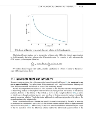
![416 CHAPTER 24 FOURIER TRANSFORM
In [1]: import matplotlib.pyplot as plt
import numpy as np
plt.style.use(seaborn-poster)
%matplotlib inline
In [2]: x = np.linspace(0, 20, 201)
y = np.sin(x)
plt.figure(figsize = (8, 6))
plt.plot(x, y, b)
plt.ylabel(Amplitude)
plt.xlabel(Location (x))
plt.show()
A sine wave can change both in time and space. If we plot the changes at various locations, each
time snapshot will be a sine wave changing with location. See the following figure with a fixed point
at x = 2.5, showing as a red dot. Of course, you can see the changes over time at specific location as
well; plot this by yourself.
In [3]: fig = plt.figure(figsize = (8,8))
times = np.arange(5)
n = len(times)
for t in times:
plt.subplot(n, 1, t+1)](https://image.slidesharecdn.com/pythonprogrammingandnumericalmethodsaguideforengineersand-231017183839-0fbc5295/85/Python_Programming_and_Numerical_Methods_A_Guide_for_Engineers_and-pdf-418-320.jpg)
![24.1 THE BASICS OF WAVES 417
y = np.sin(x + t)
plt.plot(x, y, b)
plt.plot(x[25], y [25], ro)
plt.ylim(-1.1, 1.1)
plt.ylabel(y)
plt.title(ft = {t})
plt.xlabel(location (x))
plt.tight_layout()
plt.show()
24.1.2 CHARACTERISTICS OF A WAVE
Waves can be a continuous entity both in time and space. For numerical purposes, one needs to digitize
time and space at various points. For example, in the context of geophysics, one can use sensors such
as accelerometers (which measure the acceleration of a movement) at different locations on the Earth
to monitor earthquakes; this is called spatial discretization. Similarly, these sensors usually record
the data at certain times, which is called temporal discretization. For a single wave, it has different
characteristics. See Figs. 24.1 and 24.2.
Amplitude is used to describe the difference between the maximum values to the baseline value
(see the above figures). A sine wave is a periodic signal, which means it repeats itself after a certain
time and can be measured by period. The period of a wave is the time it takes to finish the complete
cycle. In the figure, the period can be measured from the two adjacent peaks. The wavelength measures](https://image.slidesharecdn.com/pythonprogrammingandnumericalmethodsaguideforengineersand-231017183839-0fbc5295/85/Python_Programming_and_Numerical_Methods_A_Guide_for_Engineers_and-pdf-419-320.jpg)
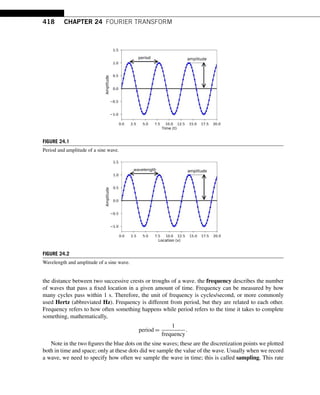
![24.1 THE BASICS OF WAVES 419
is called the sampling rate, in Hz. For example, if we sample a wave at 2 Hz, it means that at every
second we sample two data points. Now that we understand more about the basics of a wave, let us
study a sine wave, which can be represented by the following equation:
y(t) = Asin(ωt + φ)
where A is the amplitude of the wave, and ω is the angular frequency, which specifies how many
cycles occur in a second, in radians per second; φ is the phase of the signal. If T is the period of the
wave and f is the frequency of the wave, then ω has the following relationship to them:
ω =
2π
T
= 2πf.
TRY IT! Generate two sine waves with time between zero and 1 s whose frequency is 5 and 10
Hz, respectively, sampled at 100 Hz. Plot the two waves and see the difference. Count how many
cycles there are in 1 s.
In [4]: # sampling rate
sr = 100.0
# sampling interval
ts = 1.0/sr
t = np.arange(0,1,ts)
# frequency of the signal
freq = 5
y = np.sin(2*np.pi*freq*t)
plt.figure(figsize = (8, 8))
plt.subplot(211)
plt.plot(t, y, b)
plt.ylabel(Amplitude)
freq = 10
y = np.sin(2*np.pi*freq*t)
plt.subplot(212)
plt.plot(t, y, b)
plt.ylabel(Amplitude)
plt.xlabel(Time (s))
plt.show()](https://image.slidesharecdn.com/pythonprogrammingandnumericalmethodsaguideforengineersand-231017183839-0fbc5295/85/Python_Programming_and_Numerical_Methods_A_Guide_for_Engineers_and-pdf-421-320.jpg)
![420 CHAPTER 24 FOURIER TRANSFORM
TRY IT! Generate two sine waves with time between zero and 1 s. Both waves have a frequency
of 5 Hz, sampled at 100 Hz, but their phase are zero and 10, respectively. The amplitudes of the
two waves are 5 and 10, respectively. Plot the two waves and see the difference.
In [5]: # frequency of the signal
freq = 5
y = 5*np.sin(2*np.pi*freq*t)
plt.figure(figsize = (8, 8))
plt.subplot(211)
plt.plot(t, y, b)
plt.ylabel(Amplitude)
y = 10*np.sin(2*np.pi*freq*t + 10)
plt.subplot(212)
plt.plot(t, y, b)
plt.ylabel(Amplitude)
plt.xlabel(Time (s))
plt.show()](https://image.slidesharecdn.com/pythonprogrammingandnumericalmethodsaguideforengineersand-231017183839-0fbc5295/85/Python_Programming_and_Numerical_Methods_A_Guide_for_Engineers_and-pdf-422-320.jpg)
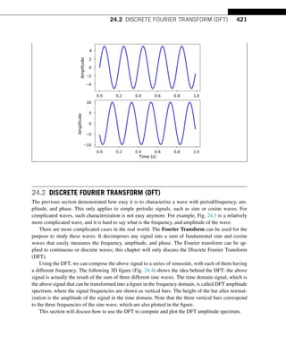
![422 CHAPTER 24 FOURIER TRANSFORM
FIGURE 24.3
More general wave form.
FIGURE 24.4
Illustration of Fourier transform with time and frequency domain signal.
24.2.1 DFT
The DFT can transform a sequence of evenly spaced signals to the information about the frequency of
all the sine waves needed to sum to obtain the time-domain signal. It is defined as
Xk =
N−1
n=0
xn · e−i2πkn/N
=
N−1
n=0
xn[cos(2πkn/N) − i · sin(2πkn/N)]
• N = number of samples
• n = current sample
• k = current frequency, where k ∈ [0,N − 1]
• xn = the sine value at sample n
• Xk = the DFT that includes information of both amplitude and phase](https://image.slidesharecdn.com/pythonprogrammingandnumericalmethodsaguideforengineersand-231017183839-0fbc5295/85/Python_Programming_and_Numerical_Methods_A_Guide_for_Engineers_and-pdf-424-320.jpg)
![24.2 DISCRETE FOURIER TRANSFORM (DFT) 423
Also, the last expression in the above equation is derived from the Euler’s formula, which links the
trigonometric functions to the complex exponential function: ei·x = cosx + i · sinx.
Due to the nature of the transform, X0 =
N−1
n=0 xn. If N is an odd number, the elements
X1,X2,...,X(N−1)/2 contain the positive frequency terms, and the elements X(N+1)/2,...,XN−1
contain the negative frequency terms, in order of decreasingly negative frequency. If N is even, the
elements X1,X2,...,XN/2−1 contain the positive frequency terms, and the elements XN/2,...,XN−1
contain the negative frequency terms, in order of decreasingly negative frequency. In the case here, our
input signal x is a real-valued sequence; therefore, the DFT output Xn for positive frequencies is the
conjugate of the values Xn for negative frequencies, and the spectrum will be symmetric. Usually, we
only plot the DFT corresponding to the positive frequencies.
Note that Xk is a complex number that encodes both the amplitude and phase information of a
complex sinusoidal component ei·2πkn/N of function xn. The amplitude and phase of the signal can be
calculated as
amp =
|Xk|
N
=
Re(Xk)2 + Im(Xk)2
N
phase = atan2(Im(Xk),Re(Xk))
where Im(Xk) and Re(Xk) are the imaginary and real parts of the complex number, and atan2 is the
two-argument form of the arctan function.
The amplitudes returned by DFT are equal to the amplitudes of the signals fed into the DFT if we
normalize them by the number of sample points. We mentioned previously that for a real-valued signal,
the output of the DFT will be mirrored about the half of the sampling rate (as shown in the following
examples). This half of the sampling rate is called the Nyquist frequency. This usually means that we
only need to look at one side of the DFT result and drop the duplicate information in the other half;
therefore, to obtain the amplitude corresponding to that of the time domain signal, we divide by N/2
instead of N.
Now that we have the basic knowledge of DFT, let us see how we can use it.
TRY IT! Generate three sine waves with frequencies 1, 4, and 7 Hz, amplitudes 3, 1, and 0.5, and
phases being all zeros. Add these three sine waves together with a sampling rate of 100 Hz; it is
the same signal shown at the beginning of the section.
In [1]: import matplotlib.pyplot as plt
import numpy as np
plt.style.use(seaborn-poster)
%matplotlib inline
In [2]: # sampling rate
sr = 100
# sampling interval
ts = 1.0/sr](https://image.slidesharecdn.com/pythonprogrammingandnumericalmethodsaguideforengineersand-231017183839-0fbc5295/85/Python_Programming_and_Numerical_Methods_A_Guide_for_Engineers_and-pdf-425-320.jpg)
![424 CHAPTER 24 FOURIER TRANSFORM
t = np.arange(0,1,ts)
freq = 1.
x = 3*np.sin(2*np.pi*freq*t)
freq = 4
x += np.sin(2*np.pi*freq*t)
freq = 7
x += 0.5* np.sin(2*np.pi*freq*t)
plt.figure(figsize = (8, 6))
plt.plot(t, x, r)
plt.ylabel(Amplitude)
plt.show()
TRY IT! Write a function DFT(x) which takes in one argument, x, with a 1D real-valued signal.
The function will calculate the DFT of the signal and return the DFT values. Apply this function
to the signal we generated above and plot the result.
In [3]: def DFT(x):
Function to calculate the
discrete Fourier Transform
of a 1D real-valued signal x
N = len(x)](https://image.slidesharecdn.com/pythonprogrammingandnumericalmethodsaguideforengineersand-231017183839-0fbc5295/85/Python_Programming_and_Numerical_Methods_A_Guide_for_Engineers_and-pdf-426-320.jpg)
![24.2 DISCRETE FOURIER TRANSFORM (DFT) 425
n = np.arange(N)
k = n.reshape((N, 1))
e = np.exp(-2j * np.pi * k * n / N)
X = np.dot(e, x)
return X
In [4]: X = DFT(x)
# calculate the frequency
N = len(X)
n = np.arange(N)
T = N/sr
freq = n/T
plt.figure(figsize = (8, 6))
plt.stem(freq, abs(X), b, markerfmt= , basefmt=-b)
plt.xlabel(Freq (Hz))
plt.ylabel(DFT Amplitude |X(freq)|)
plt.show()
Note that the output of the DFT is symmetric at half of the sampling rate (try different sampling
rates for fun). As mentioned earlier, this half of the sampling rate is called the Nyquist frequency or
the folding frequency. It is named after the electrical engineer Harry Nyquist. He and Claude Shannon
formulated the Nyquist–Shannon sampling theorem, which states that a signal sampled at a rate can be
fully reconstructed if it contains only frequency components below half that sampling frequency; thus,
the highest frequency output from the DFT is half the sampling rate.](https://image.slidesharecdn.com/pythonprogrammingandnumericalmethodsaguideforengineersand-231017183839-0fbc5295/85/Python_Programming_and_Numerical_Methods_A_Guide_for_Engineers_and-pdf-427-320.jpg)
![426 CHAPTER 24 FOURIER TRANSFORM
In [5]: n_oneside = N//2
# get the one side frequency
f_oneside = freq[:n_oneside]
# normalize the amplitude
X_oneside =X[:n_oneside]/n_oneside
plt.figure(figsize = (12, 6))
plt.subplot(121)
plt.stem(f_oneside, abs(X_oneside), b, markerfmt= , basefmt=-b)
plt.xlabel(Freq (Hz))
plt.ylabel(DFT Amplitude |X(freq)|)
plt.subplot(122)
plt.stem(f_oneside, abs(X_oneside), b, markerfmt= , basefmt=-b)
plt.xlabel(Freq (Hz))
plt.xlim(0, 10)
plt.tight_layout()
plt.show()
Plotting the first half of the DFT results shows three clear peaks at frequency of 1, 4, and 7 Hz,
with amplitude 3, 1, 0.5, as expected. This is how we can use the DFT to analyze an arbitrary signal by
decomposing it into simple sine waves.
24.2.2 THE INVERSE DFT
We can easily compute the inverse transform of the DFT:
xn =
1
N
N−1
k=0
Xk · ei·2πkn/N
.
We will leave this as an exercise for you to write a function.](https://image.slidesharecdn.com/pythonprogrammingandnumericalmethodsaguideforengineersand-231017183839-0fbc5295/85/Python_Programming_and_Numerical_Methods_A_Guide_for_Engineers_and-pdf-428-320.jpg)
![24.2 DISCRETE FOURIER TRANSFORM (DFT) 427
24.2.3 THE LIMIT OF DFT
The main issue with the above DFT implementation is that it is not efficient if we have a signal with
many data points. It may take a long time to compute the DFT if the signal is large.
TRY IT Write a function to generate a simple signal with a different sampling rate, and see the
difference in computing time by varying the sampling rate.
In [6]: def gen_sig(sr):
function to generate
a simple 1D signal with
different sampling rate
ts = 1.0/sr
t = np.arange(0,1,ts)
freq = 1.
x = 3*np.sin(2*np.pi*freq*t)
return x
In [7]: # sampling rate =2000
sr = 2000
%timeit DFT(gen_sig(sr))
120 ms ± 8.27 ms per loop (mean ± std. dev. of 7 runs, 10 loops each)
In [8]: # sampling rate 20000
sr = 20000
%timeit DFT(gen_sig(sr))
15.9 s ± 1.51 s per loop (mean ±std. dev. of 7 runs, 1 loop each)
The increasing number of data points will require a lot of computation time using this DFT. Luckily,
the Fast Fourier Transform (FFT), popularized by Cooley and Tukey in their 1965 paper,1 can solve
this problem efficiently. This is the topic for the next section.
1 http://www.ams.org/journals/mcom/1965-19-090/S0025-5718-1965-0178586-1/.](https://image.slidesharecdn.com/pythonprogrammingandnumericalmethodsaguideforengineersand-231017183839-0fbc5295/85/Python_Programming_and_Numerical_Methods_A_Guide_for_Engineers_and-pdf-429-320.jpg)
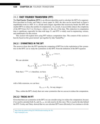
![24.3 FAST FOURIER TRANSFORM (FFT) 429
the problem into smaller ones. Let us first divide the whole series into two parts, i.e., the even and odd
number parts:
Xk =
N−1
n=0
xn · e−i2πkn/N
=
N/2−1
m=0
x2m · e−i2πk(2m)/N
+
N/2−1
m=0
x2m+1 · e−i2πk(2m+1)/N
=
N/2−1
m=0
x2m · e−i2πkm/(N/2)
+ e−i2πk/N
N/2−1
m=0
x2m+1 · e−i2πkm/(N/2)
.
As shown, the two smaller terms, which only have half of the size (N
2 ) in the above equation, are
two smaller DFTs. For each term, the 0 ≤ m ≤ N
2 , but 0 ≤ k ≤ N; therefore, half of the values will be
the same due to the symmetry properties described above. Thus, we only need to calculate half of the
fields in each term. Of course, we can continue to divide each term into half with the even and odd
values until it reaches the last two numbers, at which point the calculation will be really simple.
This is how FFT works using this recursive approach. Let us perform a quick and dirty implemen-
tation of the FFT. Note that the input signal to FFT should have a length of power of 2. If it is not, then
we need to fill up zeros to the next power of 2 size.
In [1]: import matplotlib.pyplot as plt
import numpy as np
plt.style.use(seaborn-poster)
%matplotlib inline
In [2]: def FFT(x):
A recursive implementation of
the 1D Cooley-Tukey FFT, the
input should have a length of
power of 2.
N = len(x)
if N == 1:
return x
else:
X_even = FFT(x[::2])
X_odd = FFT(x[1::2])
factor = np.exp(-2j*np.pi*np.arange(N)/ N)](https://image.slidesharecdn.com/pythonprogrammingandnumericalmethodsaguideforengineersand-231017183839-0fbc5295/85/Python_Programming_and_Numerical_Methods_A_Guide_for_Engineers_and-pdf-431-320.jpg)
![430 CHAPTER 24 FOURIER TRANSFORM
X = np.concatenate(
[X_even+factor[:int(N/2)]*X_odd,
X_even+factor[int(N/2):]*X_odd])
return X
In [3]: # sampling rate
sr = 128
# sampling interval
ts = 1.0/sr
t = np.arange(0,1,ts)
freq = 1.
x = 3*np.sin(2*np.pi*freq*t)
freq = 4
x += np.sin(2*np.pi*freq*t)
freq = 7
x += 0.5* np.sin(2*np.pi*freq*t)
plt.figure(figsize = (8, 6))
plt.plot(t, x, r)
plt.ylabel(Amplitude)
plt.show()](https://image.slidesharecdn.com/pythonprogrammingandnumericalmethodsaguideforengineersand-231017183839-0fbc5295/85/Python_Programming_and_Numerical_Methods_A_Guide_for_Engineers_and-pdf-432-320.jpg)
![24.3 FAST FOURIER TRANSFORM (FFT) 431
TRY IT! Use the FFT function to calculate the Fourier transform of the above signal. Plot the
amplitude spectrum for both the two- and one-sided frequencies.
In [4]: X=FFT(x)
# calculate the frequency
N = len(X)
n = np.arange(N)
T = N/sr
freq = n/T
plt.figure(figsize = (12, 6))
plt.subplot(121)
plt.stem(freq, abs(X), b, markerfmt= , basefmt=-b)
plt.xlabel(Freq (Hz))
plt.ylabel(FFT Amplitude |X(freq)|)
# Get the one-sided spectrum
n_oneside = N//2
# get the one side frequency
f_oneside = freq[:n_oneside]
# normalize the amplitude
X_oneside =X[:n_oneside]/n_oneside
plt.subplot(122)
plt.stem(f_oneside, abs(X_oneside), b, markerfmt= , basefmt=-b)
plt.xlabel(Freq (Hz))
plt.ylabel(Normalized FFT Amplitude |X(freq)|)
plt.tight_layout()
plt.show()](https://image.slidesharecdn.com/pythonprogrammingandnumericalmethodsaguideforengineersand-231017183839-0fbc5295/85/Python_Programming_and_Numerical_Methods_A_Guide_for_Engineers_and-pdf-433-320.jpg)
![432 CHAPTER 24 FOURIER TRANSFORM
TRY IT! Generate a simple signal of length 2048, and record the time it will take to run the FFT;
compare the speed with the DFT.
In [5]: def gen_sig(sr):
function to generate
a simple 1D signal with
different sampling rate
ts = 1.0/sr
t = np.arange(0,1,ts)
freq = 1.
x = 3*np.sin(2*np.pi*freq*t)
return x
In [6]: # sampling rate =2048
sr = 2048
%timeit FFT(gen_sig(sr))
16.9 ms ± 1.3 ms per loop (mean ± std. dev. of 7 runs, 100 loops each)
Thus, for a signal with length 2048 (about 2000), this implementation of FFT uses 16.9 ms instead
of 120 ms using DFT. Note that there are lots of ways to optimize the FFT implementation to make it
faster. The next section will introduce the Python built-in FFT functions, which will run much faster.
24.4 FFT IN PYTHON
Python has very mature FFT functions both in NumPy and SciPy. This section will take a look at both
packages and see how easily they can be incorporated in our work. Let us use the signal generated
above to run the test as shown in Fig. 24.5.
24.4.1 FFT IN NUMPY
EXAMPLE: Us the fft and ifft functions from NumPy to calculate the FFT amplitude spectrum
and inverse FFT to obtain the original signal. Plot both results. Time the fft function using this
2000-length signal.
In [3]: from numpy.fft import fft, ifft
X = fft(x)](https://image.slidesharecdn.com/pythonprogrammingandnumericalmethodsaguideforengineersand-231017183839-0fbc5295/85/Python_Programming_and_Numerical_Methods_A_Guide_for_Engineers_and-pdf-434-320.jpg)
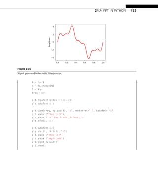
![434 CHAPTER 24 FOURIER TRANSFORM
In [4]: %timeit fft(x)
42.3 µs ± 5.03 µs per loop (mean ± std. dev. of 7 runs, 10000 loops each)
24.4.2 FFT IN SCIPY
EXAMPLE: Use fft and ifft functions from SciPy to calculate the FFT amplitude spectrum
and inverse FFT to obtain the original signal. Plot both results. Time the fft function using this
2000-length signal.
In [5]: from scipy.fftpack import fft, ifft
X = fft(x)
plt.figure(figsize = (12, 6))
plt.subplot(121)
plt.stem(freq, np.abs(X), b, markerfmt= , basefmt=-b)
plt.xlabel(Freq (Hz))
plt.ylabel(FFT Amplitude |X(freq)|)
plt.xlim(0, 10)
plt.subplot(122)
plt.plot(t, ifft(X), r)
plt.xlabel(Time (s))
plt.ylabel(Amplitude)
plt.tight_layout()
plt.show()](https://image.slidesharecdn.com/pythonprogrammingandnumericalmethodsaguideforengineersand-231017183839-0fbc5295/85/Python_Programming_and_Numerical_Methods_A_Guide_for_Engineers_and-pdf-436-320.jpg)
![24.4 FFT IN PYTHON 435
In [6]: %timeit fft(x)
12.6 µs ± 222 ns per loop (mean ± std. dev. of 7 runs, 100000 loops each)
Note that the built-in FFT functions are much faster and easier to use, especially when using the
SciPy version. Here are the results for comparison:
• Implemented DFT: 120 ms
• Implemented FFT: 16.9 ms
• NumPy FFT: 42.3 µs
• SciPy FFT: 12.6 µs
24.4.3 MORE EXAMPLES
More examples how to use FFT in real-world applications are shown below.
24.4.3.1 Electricity Demand in California
First, we explore the electricity demand from California from 2019-11-30 to 2019-12-30. You can
download data from US Energy Information Administration.4 Herein, the data has been downloaded
for you.
The electricity demand data from California is stored in “930-data-export.csv” in 3 columns. Re-
member that we learned how to read CSV file using NumPy. Here, we will use another package, pandas,
which is a very popular package that deals with time series data. This package will not be discussed
herein. We highly recommend learning how to use it by yourself.
First, let us study the data.
In [7]: import pandas as pd
The read_csv function will read the CSV file. Pay attention to the parse_dates parameter, which
will find the date and time in column one. The data will be read into a panda DataFrame, and
4 https://www.eia.gov/beta/electricity/gridmonitor/dashboard/electric_overview/US48/US48.](https://image.slidesharecdn.com/pythonprogrammingandnumericalmethodsaguideforengineersand-231017183839-0fbc5295/85/Python_Programming_and_Numerical_Methods_A_Guide_for_Engineers_and-pdf-437-320.jpg)
![436 CHAPTER 24 FOURIER TRANSFORM
we use df to store it. Then we will change the header in the original file to something easier to
use.
In [8]: df = pd.read_csv(./data/930-data-export.csv,
delimiter=,, parse_dates=[1])
df.rename(columns={Timestamp (Hour Ending):hour,
Total CAL Demand (MWh):demand},
inplace=True)
By plotting the data, we see how the electricity demand changes over time.
In [9]: plt.figure(figsize = (12, 6))
plt.plot(df[hour], df[demand])
plt.xlabel(Datetime)
plt.ylabel(California electricity demand (MWh))
plt.xticks(rotation=25)
plt.show()
From the plotted time series, it is hard to discern if there are any patterns behind the data. Let us
transform the data into frequency domain and see if there is anything interesting.
In [10]: X = fft(df[demand])
N = len(X)
n = np.arange(N)
# get the sampling rate
sr = 1 / (60*60)
T = N/sr
freq = n/T
# Get the one-sided spectrum
n_oneside = N//2](https://image.slidesharecdn.com/pythonprogrammingandnumericalmethodsaguideforengineersand-231017183839-0fbc5295/85/Python_Programming_and_Numerical_Methods_A_Guide_for_Engineers_and-pdf-438-320.jpg)
![24.4 FFT IN PYTHON 437
# get the one side frequency
f_oneside = freq[:n_oneside]
plt.figure(figsize = (12, 6))
plt.plot(f_oneside, np.abs(X[:n_oneside]), b)
plt.xlabel(Freq (Hz))
plt.ylabel(FFT Amplitude |X(freq)|)
plt.show()
Note the clear peaks in the FFT amplitude figure, but it is hard to tell what they are in terms of
frequency. Let us plot the results using hours and highlight some of the hours associated with the
peaks.
In [11]: # convert frequency to hour
t_h = 1/f_oneside / (60 * 60)
plt.figure(figsize=(12,6))
plt.plot(t_h, np.abs(X[:n_oneside])/n_oneside)
plt.xticks([12, 24, 84, 168])
plt.xlim(0, 200)
plt.xlabel(Period ($hour$))
plt.show()](https://image.slidesharecdn.com/pythonprogrammingandnumericalmethodsaguideforengineersand-231017183839-0fbc5295/85/Python_Programming_and_Numerical_Methods_A_Guide_for_Engineers_and-pdf-439-320.jpg)
![438 CHAPTER 24 FOURIER TRANSFORM
We can now see some interesting patterns, i.e., three peaks associated with 12, 24, and 84 hours.
These peaks mean that we see some repeating signal every 12, 24, and 84 hours. This makes sense
and corresponds to our human activity pattern. The FFT can help us understand some of the repeating
signals in our physical world.
24.4.3.2 Filtering a Signal in Frequency Domain
Filtering is a process in signal processing to remove unwanted parts of the signal within certain fre-
quency range. Low-pass filters remove all signals above certain cut-off frequency; high-pass filters do
the opposite. Combining low- and high-pass filters allows constructing a band-pass filter, which means
we only keep the signals within a pair of frequencies. Using FFT, we can easily do this. Let us play with
the following example to illustrate the basics of a band-pass filter. Note that we just want to show the
idea of filtering using very basic operations, in reality, filtering processes are much more sophisticated.
EXAMPLE: Use the signal generated at the beginning of this section (the mixed sine waves with
1, 4, and 7 Hz) and high-pass filter this signal at 6 Hz. Plot the filtered signal and the FFT amplitude
before and after filtering.
In [12]: from scipy.fftpack import fftfreq
In [13]: plt.figure(figsize = (8, 6))
plt.plot(t, x, r)
plt.ylabel(Amplitude)
plt.title(Original signal)
plt.show()](https://image.slidesharecdn.com/pythonprogrammingandnumericalmethodsaguideforengineersand-231017183839-0fbc5295/85/Python_Programming_and_Numerical_Methods_A_Guide_for_Engineers_and-pdf-440-320.jpg)
![24.4 FFT IN PYTHON 439
In [14]: # FFT the signal
sig_fft = fft(x)
# copy the FFT results
sig_fft_filtered = sig_fft.copy()
# obtain the frequencies using SciPy function
freq = fftfreq(len(x), d=1./2000)
# define the cut-off frequency
cut_off = 6
# high-pass filter by assign zeros to the
# FFT amplitudes where the absolute
# frequencies smaller than the cut-off
sig_fft_filtered[np.abs(freq) cut_off] = 0
# get the filtered signal in time domain
filtered = ifft(sig_fft_filtered)
# plot the filtered signal
plt.figure(figsize = (12, 6))
plt.plot(t, filtered)
plt.xlabel(Time (s))
plt.ylabel(Amplitude)
plt.show()](https://image.slidesharecdn.com/pythonprogrammingandnumericalmethodsaguideforengineersand-231017183839-0fbc5295/85/Python_Programming_and_Numerical_Methods_A_Guide_for_Engineers_and-pdf-441-320.jpg)
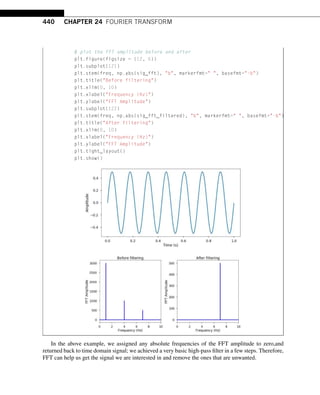
![24.5 SUMMARY AND PROBLEMS 441
24.5 SUMMARY AND PROBLEMS
24.5.1 SUMMARY
1. We learned the basics of the waves: frequency, period, amplitude, and wavelength are characteristics
of the waves.
2. The Discrete Fourier Transform (DFT) is a way to transform a signal from the time domain to the
frequency domain using the sum of a sequence of sine waves.
3. The Fast Fourier Transform (FFT) is an algorithm used to calculate the DFTs efficiently by taking
advantage of the symmetry properties in DFT.
24.5.2 PROBLEMS
1. You are asked to measure the temperature of the room for 30 days. Every day at noon you measure
the temperature and record the value. What’s the frequency of the temperature signal you get?
2. What is the relationship between the frequency and the period of a wave?
3. What is the difference between period and wavelength? What are the similarities between them?
4. What are the time domain and frequency domain representation of a signal?
5. Generate two signals: signal 1 is a sine wave with 5 Hz, amplitude 3, and phase shift 3, and signal
2 is a sine wave with 2 Hz, amplitude 2, and phase shift −2. Plot the signal for 2 s.
Test cases:
In [1]: # sampling rate
sr = 100
# sampling interval
ts = 1.0/sr
t = np.arange(0,2,ts)
freq = 5.
x = 3*np.sin(2*np.pi*freq*t + 3)
freq = 2
x += 2*np.sin(2*np.pi*freq*t - 2)
plt.figure(figsize = (8, 6))
plt.plot(t, x, r)
plt.ylabel(Amplitude)
plt.xlabel(Time (s))
plt.show()](https://image.slidesharecdn.com/pythonprogrammingandnumericalmethodsaguideforengineersand-231017183839-0fbc5295/85/Python_Programming_and_Numerical_Methods_A_Guide_for_Engineers_and-pdf-443-320.jpg)
![442 CHAPTER 24 FOURIER TRANSFORM
6. Sample the signal you generated in Problem 5 using a sampling rate 5, 10, 20, 50, and 100 Hz, and
see the differences between different sampling rates.
7. Given a signal t = [0,1,2,3], and y = [0,3,2,0], find the real DFT of X. Write the expression
for the inverse DFT. Do not use Python to find the results. Write out the equations and calculate
the values.
8. What are the amplitude and phase of the DFT values for a signal?
9. We implemented the DFT previously. Can you implement the inverse DFT in Python similarly?
10. Use the DFT function and inverse DFT we implemented, and generate the amplitude spectrum
for the signal you generated in Problem 5. Normalize the DFT amplitude to get the correct corre-
sponding time domain amplitude.
11. Can you describe the tricks used in FFT to make the computation faster?
12. Use the fft and ifft function from scipy to repeat Problem 10.
13. Add a random normal distribution noise into the signal in Problem 5 using NumPy and plot the FFT
amplitude spectrum. What do you see? The signal with noise will be shown in the following test
case.
Test case:
In [2]: np.random.seed(10)
x_noise = x + np.random.normal(0, 2, size = len(x))
plt.figure(figsize = (8, 6))
plt.plot(t, x_noise, r)
plt.ylabel(Amplitude)
plt.xlabel(Time (s))
plt.show()](https://image.slidesharecdn.com/pythonprogrammingandnumericalmethodsaguideforengineersand-231017183839-0fbc5295/85/Python_Programming_and_Numerical_Methods_A_Guide_for_Engineers_and-pdf-444-320.jpg)