1. Marc VanPuymbrouck
Lab 3
Experiments with a Large Outdoor Sand Model Aquifer
Goal and Objective
Using a large outdoor model aquifer, this lab gives a better understanding of
the relationship between vertical/horizontal variance of the sand and the hydraulic
conductivity. Measuring the different characteristics of the sand during a steady
state of flow, the heterogeneity and spatial distribution effects on the hydraulic
conductivity will be examined to understand the characteristics of each location’s
hydraulic conductivity through this aquifer in particular. Interpreting the results
obtained via the experiment, the horizontal and vertical variation of the medium can
be investigated and explanations for these variations will conducted. Understanding
how the K, or hydraulic conductivity of the medium changes with depth or distance
gives the necessary values to create statistical data and evidence of a relationship or
lack of relationship is found.
Methods
Using a large polycarbonate tanked filled with sand that is saturated with
water from a pump at the bottom of the tank, 15 piezometer are placed at different
depths and distributed throughout the aquifer. After a steady state is established
using a pump, the depth of the water in each piezometer is found using a measuring
tape sent down the tube that alerts the user at what depth the water is found. The
outflow of the pump is determined using a timer and collecting the flowing water
into a measurable container. An example being filling a 20-liter bucket with the

2. flowing water, recording the time it took to fill the bucket will give you the outflow
of the aquifer. The rate of the flow is then changed, either increased or decreased
and once a steady state is achieved, finding the outflow and depth to water is
conducted again for a second trial. The height of the water and sand are found.
Once these values are found, calculating the area of the aquifer, the
differences in the hydraulic gradient, and the outflow will supply enough
information to apply Darcy’s Law; K=Q/A*dl/dh. Finding the hydraulic conductivity
through these means allows comparisons between the K values with a change in
flow, location, and depth. Q was found through the filling of the measurable
container through a time trial. A is found by multiply the width by height, or A=w*l.
The dl is found through the distance between each piezometer location. Finding the
difference in the height of the Mid-Screen elevation (ft) from location to location
results in the dl. For the C location, the difference in Mid-Screen elevation and
Height of the Water (ft) is found. Finding the dh is finding the difference in Heads.
To find the Head (ft) in each piezometer the difference between the Top Elevation
and Depth to Water (ft) gives you three heads for the three locations, located in the
five wells. The difference of the Head (ft), location to location results in finding the
dl. In the case of C locations, the difference in head and the height of the sand is
taken. This gives you all the variables needed to determine the hydraulic
conductivity, or K. The values found in table 3 were determined through the
program Statplus, where a Descriptive Statistical analyses was conducted. To find
the values in figures 3 and 4 a Regression Test was run, and to find the values in
table 4 a T-test was ran. The values for tables 7 and 8 could be determined through

3. finding the standard deviation of the Hydraulic Conductivity (ft) for both trials,
where the mean is subtracted from each K value, squared, then the mean of the
squared values is found and the square root is taken.
Results
Table 1 reportthe Hydraulic Conductivity (ft/day) and Hydraulic Gradient (ft/day) for various depths
(ft) between each well in relationship to the sand/water interface.
Well Location
K (Ft/Day) Trial
1
K (Ft/Day) Trial
2
Hydraulic
Gradient
Trial 1
Hydraulic
Gradient
Trial 2 Depth(Ft)
1 A to B 192.19 246.29 0.16 0.05 5.34
1 B to C 124.52 125.72 0.25 0.1 3.47
1
C to sand
surface 62.66 55.32 0.49 0.24 1.34
2 A to B 216.89 179.13 0.14 0.07 5.59
2 B to C 113.59 115.25 0.27 0.11 3.54
2
C to sand
surface 70.17 66.87 0.44 0.19 1.44
3 A to B 170 167.93 0.18 0.08 5.48
3 B to C 108.19 104.86 0.29 0.13 3.44
3
C to sand
surface 71.37 65.86 0.43 0.2 1.36
4 A to B 145.17 156.67 0.21 0.08 5.41
4 B to C 108.51 89.27 0.28 0.15 3.15
4
C to sand
surface 73.15 88.54 0.42 0.15 1.32
5 A to B 164.45 120.42 0.19 0.11 5.48
5 B to C 100.76 89.27 0.31 0.15 3.5
5
C to sand
surface 85.89 114.15 0.36 0.12 1.64

4. Table 2 shows theQ/flow of water for both trials (ft3/second), height of the water (ft) in the aquifer,
height of the sand (ft) in the aquifer, and the area (ft) of the aquifer.
Test1 Q
(ft3/sec)
Test2 Q
(ft3/sec)
Heightof
Water (ft)
Heightof
Sand (ft) Area(ft)
0.018 0.0077 10.58 9.56 50.27
The results, (table 1) are the values gathered by testing the Hydraulic
Conductivity (ft/day) and Hydraulic Gradient for the outside aquifer at two different
speeds of flow shown in table 2 (ft3/day). By collecting the depth of the water (ft)
by using a measuring tape with intervals in inches dropped down the piezometers
labeled “wells”.
Discussion
The results of this experiment show that there are significant changes in the
hydraulic conductivity between the two trials. The data found through the
experiment allows for the characteristics of this aquifer to be examined both
vertically and horizontally, understanding how water flows through the medium.

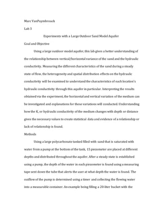
5. Figure1 is a histogram that shows the distributionof the observations seen in trial 1 of the experiment.
The K values (ft/day) are categorized withinintervals of 20 to show the trends of variance.
Figure2 is a histogram that shows the distributionof the observations seen in trial 2 of the experiment.
The K values (ft/day) are categorized withinintervals of 20 to show the trends of variance.
Table 3 show various ways in which the two trials Hydraulic Conductivity werecharacterized, including
the mean K (ft/day), Standard Deviation (ft/day), Range (ft/day, Standard Deviation (ft/day), and 95%
Confidence Interval (ft/day)
Mean
K
(ft/day)
Standard
Deviation
(ft/day) Range (ft/day) StandardError (ft/day)
95%
Confidence
Interval
(ft/day)
GeometricMean
(ft/day)
120.5 47.74 154.24 12.36 108.14,132.87 112.15
109.95 38.09 123.81 10.18 99.77, 120.13 103.83
The overall distribution of hydraulic conductivity for each of the trials is
significantly different, indicating that the change in flow, or Q, (table 2) affects the
hydraulic conductivity of the aquifer. Recognizing that Darcy’s Law can be followed
for both trials by the regression equation, (figures 3/4) and that a laminar flow must

6. occur in the aquifer, allows comparisons between the two trials to be made. For
trial 1 most K values are 60-80 ft/day, or 100-120 ft/day, (figure 1). All locations A
to B have values higher than the mean of 120, and all but one locations that are
either B to C or C to surface are less than 120, (table 1). The mean is skewed to the
right because of values found at well 1, location A to B which has a K value of 192.19
pulling the medium up to 120. A more accurate description of the distribution of the
hydraulic conductivity would come from the Geometric Mean (ft/day), which
indicates the central tendencies/values and help prevent large values from having a
disproportional effect. This mean, (table 3) better shows that a majority of the K
values are closer to 100-120, which more accurately describes the distribution.
Compare these numbers to trial 2, (figure 2) the slower flow rate creates an aquifer
with a more consistent hydraulic conductivity. Looking at the differences between
the geometric mean and standard mean of both trials’ hydraulic conductivity, (table
3) the lesser difference between the two means in trial 2 indicates a lower amount
of variance. This can be confirmed by looking at the lower Standard Deviation, and a
smaller Standard Error that in turns creates a tighter Confidence Interval, (table 3).
The geometric mean for both fall within the 95 % confidence interval found using
the standard error, demonstrating that this mean accurately represents the values.
The resulting bell shaped curve that is created from more consistent hydraulic
conductivity in trial 2 points to the conclusion that a slower flow rate will result in a
more steady hydraulic conductivity throughout the aquifer, and that a faster flow
rate will result in hydraulic conductivity with a large range and uneven distribution.

7. Figure3 shows the relationship between the depth (ft) and the Hydraulic Conductivity (ft/day).,
reporting the regressionequation, R2 value, and P-Value in the firsttrial
Figure4 shows the relationship between the depth (ft) and the Hydraulic Conductivity (ft/day, reporting
the regressionequation, R2 value, and P-Value in the second trial.
Table 4 shows therelationship between the depths P-value using a T-trial, or comparisontrial. Shortto
medium aredepths are 1-3ft, Medium to Deep are 3ft-5ft, and Short to Deep depths are 5ft-1ft.
Depths(ft) P-Value Trial 1 P-Value Trial 2
Short to
Medium 0.00035 0.27
Mediumto
Deep 0.00511 0.00743
Short to Deep 0.00073 0.0055
The heterogeneity of the system can be observed through the change in hydraulic
conductivity with a change in depth. Measuring the height of water in the

8. piezometer wells resulted in finding the head of each section of the aquifer, evenly
distributed throughout the 5 well locations. Using Darcy’s law, the change in head
and depth can be converted to dh/dl, which can be applied to find the hydraulic
conductivity for the depths in each well. In both trials, (figures 3/4) a significant
relationship between the increase in depth and the increase in hydraulic
conductivity is found. The linear equation validates that Darcy’s law was followed
and the P-values for both trials were determined lower than .01 giving strong
evidence against the Null Hypothesis that proves there is a correlation between the
depth and K-value. The similarities between the two trials indicate that a change in
flow rate does not control the hydraulic conductivity and that the Effective Porosity
plays a larger role within the system. The deeper/middle parts of the aquifer that
have high hydraulic conductivity change to a shallower, less permeable section
towards the top of the medium that describes the geologic make up of the material
in this section. The top of the aquifer, C to surface, has low hydraulic conductivity
that leads this study to believe the shallower locations are made up of clay/organic
material, which has very low permeability. Clay could cause the low hydraulic
conductivity of liquid in these locations and the increase of hydraulic conductivity
seen as the depths increase, (figure 3/4) indicate a material with a higher
permeability. A higher amount of hydraulic conductivity as the depths of the aquifer
increase are characteristics of sands similar to sandstone or limestone material.
The P-values of the experiment, (table 4) mirror the relationship of the hydraulic
conductivity and depth. The three different distances, (A, B, C) grouped together by
locations between the piezometers can have their probabilities determined through

9. a T-test, which finds the P-value, measuring the evidence against the Null
Hypothesis or that the results show no relationship between the two points of
measurement. This gives valuable information in regards to why the P-value for trial
1 is so much lower than that of trial 2, (figures 3/4). Very strong evidence against
the Null Hypothesis is found in all comparisons of locations, (table 4), except for trial
2’s “short to medium”. Looking back at the K values, (table 1) there seems to be an
abnormality in well 5, C to surface value, which is listed at 114 (ft/day). This value is
well above the mean of C to surface, (table 7) and is well beyond the Standard
Deviation of 20.99 (ft/day) whose deviation is only that high because of the
resulting value. It is an outlier created by human error, which can be found in the
initial value of K for this specific piezometer. Looking at the dl for C to Surface well
5, (table 1) it is considerably higher than any other value of dl in any C to Surface
location. With the change in dl having significant strength over the hydraulic
conductivity, this is where the error occurred. The Bottom Elevation, (table 1) for
this location is much more than any other C to Surface value, concluding an error in
the measurement must have occurred.
Table 5 reports change in the average Hydraulic Conductivity (ft/day) and depth (ft) between the five
wells for trial 1.
Well Average K(Ft/Day) Average Depth(ft)
1 126.46 3.38
2 133.56 3.52
3 116.52 3.43
4 108.95 3.29
5 117.03 3.54

10. Figure5 shows the difference between the five wells Hydraulic Conductivity (ft/day) and depth (ft) for
trial 1.
Table 6 reports change in the average Hydraulic Conductivity (ft/day) and depth (ft) between the five
wells for trial 2.
Well Average K(Ft/Day) Average Depth (ft)
1 142.45 3.38
2 120.41 3.52
3 112.88 3.43
4 111.49 3.29
5 107.95 3.54
Figure6 shows the difference between the five wells Hydraulic Conductivity (ft/day) and depth (ft) for
trial 2.

11. The data obtained through the experiment shows a lack of a horizontal relationship
between the location in the piezometer and the hydraulic conductivity, (figure 4/5
and tables 4/5). The depths for each well and the 5 different locations where the
piezometers are located have no significant pattern, which allows assumption to be
made that there is no relationship between the location horizontal of the wells and
the hydraulic conductivity.
Table 7 show the variance amongst the locations Hydraulic Conductivity (ft/day) using each Standard
Deviation (ft/day) and Range (ft/day) for trial 1.
Location
Mean K
(Ft/Day)
StandardDeviation
(Ft/Day)
Range
(Ft/Day)
Depths
(Ft)
A to B 177.74 24.66 71.72 5.46
B to C 111.113 7.85 23.76 3.42
C to
Surface 72.65 7.53 23.23 1.42
Table 8 show the variance amongst the locations Hydraulic Conductivity (ft/day) using each Standard
Deviation (ft/day) and Range (ft/day) for trial 2.
Location
Mean K
(Ft/Day)
StandardDeviation
(Ft/Day)
Range
(Ft/Day) Depth(Ft)
A to B 174.09 41.14 125.88 5.46
B to C 104.87 14.35 36.45 3.42
C to
Surface 78.15 20.99 58.83 1.42
Figure7 show the Standard Deviation (ft/day) for the trial 1.

12. The changing variance of the aquifer can be determined through the change
in Standard Deviation (ft/day) by a change in depth, (tables 7/8). It helps identify
the materials characteristics in each of the three different sections in the aquifer,
(figure 7) and how the variance of the hydraulic conductivity is different with a
change in depth. While the more shallow of the two locations have relatively low
standard deviation in both trials, (table 7/8) a high level of variance is seen in the
deepest location, A to B. Even with the skewed data found from trial 2’s C to surface,
standard deviation still has a smaller value than that of A to B. This could be due to
the hydraulic conductivity of B to C and C to Surface being closer to one another,
(table 1) with a larger difference between B to C/C to Surface than A to B/B to C.
The data presented, (figure 7) shows the change from the higher elevation
locations to lower elevation locations has a dramatic change in hydraulic
conductivity, oppose to a gradual increase of standard deviation. This characteristic
has an important role in determining the sorting of the sands in the three locations.
Low variance is associated with sediments that are very well sorted and uniformed,
while high variance is associated with sediments that are poorly sorted and not
uniform. The high variance of the A to B location not only points to a poorly sorted
sediment, but that there must be a large change in the sorting from location A to B
and B to C due to the dramatic change in standard deviation, (figure 7). The much
lower variance in these two layers, in particular C to Surface is a key characteristic
of clay materials. Clay has very small grain sizes, which usually means the material
will be well to very well sorted. This reinforces the results of the change in hydraulic
conductivity with a change in depth, (figures 3/4) which the top locations are made

13. of clay/organic material. The much higher and dramatic change in variance
indicates that the lower section of the sediment has characteristics of
sandstone/limestone.
The figures derived from this lab’s results give the necessary information to
determine the heterogeneity of1 the system. While the horizontal variance had no
measurable trends, the vertical variance in the system helps determine the
geological make up. A high hydraulic conductivity towards the bottom of the aquifer,
with a lower hydraulic conductivity towards the top of the aquifer, points to an
upper layer of sediment being comprised mostly of clay that has low hydraulic
conductivity. The increase in hydraulic conductivity with an increase in depth
illustrates the change from clay sediment to sands more similar to sand or
limestone, both that have high hydraulic conductivity. These findings are reinforced
by the high variance of the deeper locations, indicating poorly sorted material,
another characteristic of sand or limestone. The low variance of the top locations in
the aquifer fit with these findings, that clay is very well sorted and in-turn has low
variance.