Jwrhe10065 20150204-144509-1366-46826

Journal of Water Resource and Hydraulic Engineering Jan. 2015, Vol.4, Iss. 1-4, PP. 9-22
- 9 -
Multi-Aquifer Parameterization with well loss in Ver-
tical Flows
P.K.Majumdar
Professor, Civil Engineering Department, AKS University, Satna, MP, India
Email:patmajum@yahoo.com
Abstract-Usually aquifer parameters are estimated through pumping/recharge test. Precondition for using those parameters in the numerical
model is to ensure the synonymy of the hydro-geological condition between the field setup and the conceptual model. In many cases, it is er-
roneous. While numerical modelling in multi-aquifer considered vertical flow in general, it was reflected in the pumping solutions only to the
extent of treating a leakage through the aquitard. As such well characterisation in multi aquifers separated by an aquiclude is illusive in the
literature. As a result of which, interconnected aquifers were considered as isolated ones in the pumping/recharge tests. Therefore, estimated
parameters were for a single aquifer, not for an aquifer connected to multi aquifers. In the present paper, the solution for a multi-aquifer
system comprising of two interconnected aquifers separated by an aquiclude is presented. Vertical flow in the well bore with well loss due to
friction has been considered. It is concluded that multi-aquifer parameters computed using present solution technique are more scientific and
economical.
Keywords: Interconnected aquifers, diffusivity ratio, well bore interaction, equivalent single aquifer, the friction parameter
I. INTRODUCTION
Neuman and Witherspoon (1969) provided the aquitard drawdown in FEM solution using Darcy’s law for groundwater flow in
the existing hydrostatic condition in a multi-aquifer system. They also encouraged the use of equivalent parameter values to resolve
issues of vertical variation of hydraulic conductivity and specific storage of the aquitard. Herrera (1970) realized the possibility of
an analytical solution to describe the vertical flow in a homogeneous aquitard using Duhamel convolution theorem. Later on Hen-
nart et al. (1981) extended it to inhomogeneous multi-aquifer system using eigen function approaches. Using discrete kernel ap-
proach, Mishra et al. (1985) analyzed the two-aquifer system. Analytical solutions developed for multi-aquifers in general catered
more to evoke the aquifer diffusivity ratios (Sokol, 1963; Wikramaratna,1984; Hemkar, 1984; Hunt,1985).
In analytical solutions, vertical flows in multi aquifers have been treated as leakage from the aquitards separating the two aqui-
fers. Hemkar (1999) developed the uniform well-face drawdown solution including the effects of a finite diameter well, wellbore
storage and thin skin. Bakker and Hemkar (2002) considered the vertical flow in the layer interfaces of the multi-aquifers. Yeh et al.
(2003) developed two layered aquifer model with skin effects. Based on the first order perturbation technique, problem of steady
groundwater flow toward a pumping well in multi-aquifer system with anisotropy of the horizontal conductivity was solved by
Meesters et al. (2004). Kim and Parizek (2004) described the Rhode effect caused by (1) a slower head recovery of the un-pumping
stress and (2) an amplification of the excessive extension in the lower part of the aquitard due to its relatively higher deformability.
They did not found extension from the pumped aquifer into the adjacent aquitard and un-pumped aquifer due to the relatively
lower hydraulic conductivity of the aquitard, Using numerical inversions of exact analytical solutions for Laplace transforms, Hunt
and Scott (2007) developed an approximate solution for flow to a well in an aquifer overlain by both an aquitard and a second aqui-
fer containing a free surface. Sedghi et al. (2009) developed Laplace domain solutions for three-dimensional groundwater flow to a
well in confined and unconfined wedge-shaped aquifers.
Numerical well flow models considered radial and vertical groundwater flow near a well since seventies. Bennet et al. (1982)
devised for the calculation of three-dimensional groundwater flow. Sudicky et al. (1995) applied finite elements to simulate well
flow in heterogeneous aquifers with wellbore storage. Xiang (1995) used a finite difference code to investigate the skin effect dur-
ing flow meter tests in layered aquifers. Neville and Tonkin (2004) reviewed four methods to represent multi-aquifer wells with the
widely used code MODFLOW (McDonald and Harbaugh, 1988) to demonstrate that results obtained with the Multi Aquifer Well
(MAW1) package closely matched exact solutions of Sokol (1963). Bakker (2006) presented an analytic element approach for the
modeling of steady groundwater flow through multi-aquifer systems with aquifer and leaky layer properties. Craig and Gracie
(2011) applied extended finite element method to the problem of transient inter-aquifer leakage through passive wellbores. Prece-
dence out of the literature, discussed above, does not guarantee the numerical model calibration of multi-aquifer system, like it
does in the case of a single aquifer. The reason behind low reliability is the model parameters, which were estimated under differ-
ent hydro-geological condition. Such inconsistency develops; firstly, due to difficulty in extending the slug or pump test solutions
of single aquifer to multi-aquifer setup. Secondly, due to the fact that the complex analytical and numerical solution exclusively

- 10 -
developed for multi-aquifers, could not be amicably adopted in the field tests. Hence in the multi aquifer tests, parameterisation
actually dealt with isolated aquifers overlooking the interconnectivity factor.
Analytical solutions are available dealing with interconnectivity between various layers of multi-aquifer, mostly limited to aq-
uifer-aquitard setups. Neuman and Witherspoon (1972) put forward the idea of putting observation wells in the over and underly-
ing aquitards for a pumping test in a multi-aquifer setup. Cheng and Morohunfola (1993) presented an analytical solution of a radi-
al flow to a pumping well at constant discharge located in a multilayered leaky aquifer system, to evaluate the drawdown at any
given time and location in any layer. Miyake et al. (2008) carried out multi-aquifer pumping tests, in multi-screen pumping well
and multi-level piezometers in multi-layered confined aquifers to estimate parameters in aquifers, and also for low permeability
layers between the aquifers, using the Cooper-Jacob method and a finite element groundwater model. Cihan et al. (2011) developed
analytical solutions accounting for the combined effect of diffuse and focused leakage to solve for pressure changes in a system of
N aquifers with alternating leaky aquitards in response to fluid injection/extraction from any number of layers. Basic ingredient to
the mathematical formulations of the above-stated solutions remained a minimum boundary condition of leakage face. In the ab-
sence of such boundary condition, solutions required numerical integration. Ruud and Kabala (1997) and Zlotnik and Zurbuchen
(2003) showed the depth wise head loss distribution in borehole flow meter test, where parameter estimation required numerical
techniques. Difficulty in adopting numerical solutions encouraged field testing in confined aquifers separated by aquiclude, to deal
with each aquifer turn by turn, packing rest of the aquifers.
Elsewhere, well bore model in Sandia Waste Isolation Flow and Transport (SWIFT) as detailed in Reeves et al. (1986) included
solution for frictional pressure drops in the wellbore as;
dp = gdz/gc + fdz (1)
Where f is related to friction factor ‘f’ through f = fu2
/2rT, where f rT/2 is the shear stress in the well bore face in the direction
of flow. For laminar flow, the friction factor is taken as f = 64 / Re; log10 (Re) 3.3; For the transition zone, f = 10x
;
3.3log10(Re)3.6, with the exponent given by the polynomial, x=260.67228.62log10(Re)+66.307 log10 (Re)2
+6.3944 log10
(Re)3
; For the turbulent flow region, the surface roughness fr of the wellbore becomes; f = f (Re, fr). The second term on the right-
hand side in equation (1), supplemented to the pressure difference between the two well skins open to successive aquifers. In the
present paper, this term is included and treated analytically for the multi-aquifer setups to address the interaction between the aqui-
fers via Darcian or non-Darcian vertical flow through the wellbore as highlighted by Chen and Jiao (1999). Well-loss characteriza-
tion in the wellbore is studied using the approach of Duhamel Convolution theorem under hydrostatic conditions. Single aquifer
solution of Majumdar et al. (2013) has been extended to two aquifer systems separated by an aquiclude. Both steady and unsteady
well water level conditions have been solved. Testing setup required for the use of the type curves generated in the present paper is
different to that exist currently, which has lead to defer field validation till the theory becomes established, and subsequently com-
mensurable methodology for field testing could be practised.
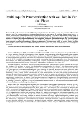
Fig. 1. Schematic diagram of the recharge well
II. SOLUTION FOR SINGLE AQUIFER

- 11 -
In Fig. 1, schematic cross-section of a fully penetrating recharge well in a single confined aquifer is shown with initial piezo-
metric head in the aquifer at a height Ha from the bottom of the aquifer. Transmissivity and storage coefficient of the aquifer are T
and S respectively. The well screen and unscreened portions have the same radius rw. For augmenting recharge, water well is filled
to a height Hw, so that piezometric water level in the aquifer goes up whereas, water level in the well starts receding. In a particular
time step n, the piezometric head in the aquifer at radial distance r from the recharge well is given by
    ),(,, nrsorHnrH aa  (2)
Here s(r, n) is the head rise in the aquifer at a radial distance r from the recharge well and given by (Morel-Seytoux and Daly,
1975)
     

n
a ntrQnrs
1
1,,,

 (3)
 1,,   ntr is known as Discrete Kernel coefficient or Delta function. Other notations are listed at the end of the paper.
Derivation of the Delta function ‘’ is included as Appendix-A, using Theis (1935) well function for the unsteady flow in a con-
fined aquifer. With friction loss in the well bore, Duhamel’s convolution equation is written as;
         
 
g
kl
r
nQ
ntrQQ
r
oHoH
w
a
a
nn
a
w
aw
2
1
1,,
1
2
2
11
2







   

 
(4)
In equation 3, k is the friction parameter (f/D), where f is the friction factor in Darcy-Weisbach equation for head loss due to
friction hf in the recharge well given by the equation 5.
gD
flv
hf
2
2
 (5)
Value of friction factor is available in Moody’s diagram (Featherstone and Nalluri, 1982) for known Reynolds number. Devel-
opment of the single aquifer solution with head loss due to friction could be followed elsewhere (Majumdar et al., 2013), where the
solution was validated with the theoretical solution of Cooper et al. (1967) and field data of Hansol injection well near Ahmedabad,
Gujarat, India. Majumdar and Mishra (2007) have documented the type curves, which require only well water level observations.
In the present article, single aquifer solution has been extended to two aquifer setups separated by an aquiclude, to discuss good
characterization in multi aquifers.
III. EXTENSION TO MULTI-AQUIFER SETUP
For the multi-aquifer setups, simultaneous equations were formulated under hydrostatic condition using Bernoulli’s theorem. A
two-layered confined aquifer with an initial head of Ha(o) is shown in Fig. 2. Aquifers have transmissivity T1 in the first aquifer
and T2 in the second, and the respective storativity values are S1 and S2. Radius of the well for both screened and unscreened por-
tion is rw. The aquifers are recharged by a fully penetrating well up to the height of HW(o). Let the quantity of water moved to first,
and second aquifers are Qa1 and Qa2 respectively. Qw is the quantity of water moved out of the well. It is required to derive expres-
sions to compute Qa1 and Qa2 for a constant head well condition and variable head conditions.
A. Constant water level in the well
Applying Bernoulli’s equation between well water level and elevation head at point 2 (at aquifer 1 top level) of a multi-aquifer
system in Fig. 2, using the notations there and k as friction factor per unit diameter of recharge well,
      121
1
1
22
1 1,,
22
hhntrQ
g
V
g
V
kloH
n
aw  


(6a)

- 12 -
   
   
    121
1
1
2
2
21
1 1,,
2
1 hhntrQ
g
r
nQnQ
kloH
n
a
w
aa
w 





 
 



(6b)
Fig. 2. Schematic diagram of recharge well in multi-aquifer setup.
Then applying same between point 3 (at aquifer 2 top level) and 2,
        
   
   
    21
1
2222
2
2
22
2
2
2
1
11
0
2
1
11
2
2
21
1
1,,
2
1
1
2
1,,
2
1
hdldntrQ
r
nQ
g
kl
dx
r
nQ
d
x
nQ
g
k
hntrQ
r
nQnQ
g
h
n
a
w
a
w
aad
n
a
w
aa








































 












(7)
Where, 1 and 2 are the Discrete Kernel coefficient or Delta function of aquifer 1 and 2 respectively. Other notations are listed
at the end of the paper.
Equations 1 and 2 are simplified in the following form,
  01,,2 1
22
 axtrbxybybx  (8)
    01,,1,, 21
22
 cytrxtrsxywyvx  (9)
where,
 nQx a1 (10)
 nQy a2 (11)
     11
1
1
112  




nQhhoHa
n
aW (12)

- 13 -
 
42
1
2
1
wrg
kl
b


 (13)
   11
1
1
1  




nQc
n
a    12
1
1
2  




nQ
n
a (14)
42
2
1
wrg
r

 (15)
42
1
2 wrg
kd
u

 (16)
 
42
2
2
1
wrg
kl
e


 (17)
 ruv  (18)






 rus 2
2
3
(19)






 eruw
3
1
(20)
For solving equations (6) and (7) Newton-Raphson method was employed.
B. Variable water level in the well
The following three equations were written for the solution of three unknowns Qa1, Qa2 and Qw for varying water level in the
well, where Qw is the change in well storage.
     nQnQnQ Waa  21
(21)
           
   
   
g
r
nQnQ
kl
gr
nQnQ
ntrQoHQ
r
Q
r
oH
w
aa
w
aa
n
aa
n n
a
w
a
w
W
22
1
1,,
11
2
2
21
12
2
21
1
1
1
1 1
2212





 





 

    





  
(22)
and
     
   
 
 
 
   
   1,,
1
22
2
1
2
1
1,,
2
1
22
2
1
11
0
2
2
2
2
2
2
2
2
2
21
1
1
1








































 












ntrQdx
r
nQ
d
x
nQ
g
k
g
r
nQ
kl
gr
nQ
oH
gr
nQnQ
ntrQoH
n
a
w
aad
w
a
w
a
a
w
aa
n
aa
(23)

- 14 -
Further simplification reduced equation 22 and 23 similar to equations 4 and 5 respectively, except the current value of Hw (o)
required to be modified every time step. Again Newton-Raphson method was applied for the solution of the set of equations to
evaluate the values of Qa1 and Qa2.
IV.RESULTS OF ANALYSIS
For the schematic single aquifer configuration of Fig. 3, illustrations depicting computation of well heads and recharge rates are
shown in Fig. 4 and Fig. 5 respectively. Values were computed using equation 4, with discrete kernel of Theis (1935) well function.
Influence of the friction parameter is well evident with well loss dissipating the well water column in Fig. 4 and non-dimensional
recharge rates in Fig. 5 much slowly. The range of friction parameters used in the analyses covered Darcian and non-Darcian flow
regimes in a well bore. The single aquifer formulation when extended to the two aquifer setup, the friction parameter generated a
difference between the piezometric head of successive aquifers, causing an interaction between the aquifers through well bore.
Interaction through the interfaces between aquifer and aquiclude was not considered. Such demonstrative analysis was carried out,
comparing the recharge well water levels in the multi-aquifer with those for an equivalent single aquifer. A hypothetical case of
two-aquifer system, each 5 m thick, separated by a 3 m thick aquiclude was considered. Confining layer of the top most aquiclude
was having a thickness of 5 m. Diameter of the well was 1.0 m. Initial water level depth was 14 m and the recharge well was
poured up to the depth of 16 m. Storage coefficient was kept constant as 0.01 and the friction factor per unit diameter of the well
was considered as zero and 1.0 respectively for respective sets of analyses.
Fig. 3. Conceptual aquifer configurations for the illustrative example.
Fig. 4. Change in well water level with friction parameter.

- 15 -
Fig. 5. Non-dimensional recharge rates for different friction parameter.
For the equivalent single aquifer, T and S values were obtained by summing the T and S values of the individual aquifers of the
multi-aquifer system, because T, S and thickness in each of the aquifers of multi-aquifer system were equal. Recharge well water
column and static water level in the multi-aquifer case and the equivalent single aquifer case were maintained at the same level.
Consequently, the aquiclude thickness between the two aquifers of multi-aquifer system was accounted in the equivalent single
aquifer thickness. In Fig. 6, results of multi-aquifer solution in case of no friction loss show a good match between the head decline
in the well for single and two-aquifer cases. In the case of friction loss (k =1) the water level in the well declined differently for
equivalent single and two-aquifer system as shown in Fig. 7, indicating nonlinear behavior arising due to well loss and subsequent
interaction between the aquifers through well bore. This behavior could be Darcian or non-Darcian, depend upon the range of k
and well radius used in the analysis. Outcome of this analysis is of paramount practical importance, as during the analysis it was
found that existing concept of equivalent single aquifer did not apply, when head loss during recharge test was accounted.
Therefore, present parameterisation techniques in multi aquifer are questionable. Incorporation of such parameters for numerical
model calibration is an added time-consuming effort due to the increase in the number of trials. Seldom calibrated parameters
could be the field tested values.
Fig. 6. Comparison of recharge well water levels for single and multi aquifer without friction loss.

- 16 -
Fig. 7. Comparison of recharge well water levels for single and multi aquifer with friction loss.
To study the effect of diffusivity between the two aquifers, different ratios ranging from 0.2 to 5.0, were tried out. Recharge
rate variations to both the aquifers under constant and variable head conditions are shown in Figs. 8 to 10 for different diffusivity
ratios. Recharge to the individual aquifer increases with the increase in the diffusivity of that particular aquifer. Accordingly the
recharge to the remaining aquifer decreases. However, there is no indication that recharge ratio between individual aquifer follows
the diffusivity proportions. In a multi-aquifer setup, type curves such as Fig. 8 to Fig. 10 could make it convenient to ascertain the
diffusivity ratios between the two aquifers. Consequently, if diffusivity of one aquifer is known using Majumdar and Mishra
(2007), parameterization for the other aquifers becomes hand calculation. When applied to model calibration, lesser trials would
be required due to synonymy in the hydro-geological conditions of the testing setup and the conceptual model. Further, field test-
ing could be carried out at much cheaper financial investments, as packers in the remaining layers are no more required.
Fig. 8. Recharge rates for aquifer diffusivity ratio (top/bottom) as 0.2.

- 17 -
Similarly, piezometric heads in the recharge well for constant and variable head conditions are shown in Fig. 11. Under the va-
riable head condition, water level in the well goes down with a steeper rate initially and subsequently gains a flatter trend with time.
It depends upon the ratio of the diffusivity of the two aquifers and the friction parameter. In Fig. 11, with the increase in the ratio of
diffusivities for the top and bottom aquifer, water level in the recharge well is improving. It is attributed to the effect of the de-
creasing total diffusivity value of the two aquifers and likely to differ in case of an overall increase in the total diffusivity value.
These exercises accounted head loss due to velocity of flow and friction in the recharge well, which caused unequal piezometric
heads in the individual aquifers at the well face. Unique feature of Duhamel’s convolution theorem allowed coupling of momentum
with mass balance in the recharge well. Present formulation estimates unsteady recharge to the individual aquifers under current
wellhead condition. Flexibility in transforming the head into a flux and vice-versa at the well face makes it possible to generate
pressure and recharge solutions simultaneously but successively. Algorithm-wise, present exact solution satisfies the conservation

- 18 -
of mass and momentum in an identical manner with which an approximate solution derives boundary conditions in the numerical
methods. Therefore, present solution technique could be termed as semi-analytical rather than strictly analytical. Although concep-
tually the results were verified, however, it could not be compared with the field observation, mainly due to the absence of recon-
cilable testing methodology. Present accurate solutions are simple to adopt for parameterization of multi-aquifer setups with much
cheaper experimental setup, not warranting the use of packers anymore.
Fig. 11. Recharge well water levels for different aquifer diffusivity ratios.
V. CONCLUSIONS
In the present paper, the semi-analytical solution for a single aquifer is extended to the two-layered aquifer system for both con-
stant and variable wellhead conditions. With the incorporation of head loss due to friction in the recharge well, aquifer-to-aquifer
interaction through well bore was formulated and established in an exact solution in a way, similar to that of numerical models.
Solution technique is flexible and can be extended to the systems comprising of any number of aquifers separated by suitable num-
bers of aquicludes. Parameter estimation through present solution will ensure precision along-with time and cost effectiveness.
More importantly, estimated parameters have a scope of reconciling with the field conditions, when used for the model develop-
ment, using numerical methods. Model calibration is expected to be much smoother.
Notations
Ha = Height of piezometric level above datum (L)
Hw = Height of well water level above datum (L)
d1, d2 = Aquifer thickness (L)
l1, l2 = Aquiclude thickness (L)
rw = Well radius (L)
rc = Well casing radius (L)
r = Radial coordinate (L)
D = Well bore diameter (L)
hf = Head loss due to friction (L)
S = Storativity (ratio)

- 19 -
T = Transmissivity (L2
/T)
Qa = Rate of recharge at well face (L3
/T)
Qr = Rate of injection (L3
/T)
Qw = Change in well storage (L3
/T)
v = Darcy flux (L3
/T)
δ = Discrete Kernel (L/(L3
/T))
f = Friction factor (non-dimensional)
g = Acceleration due to gravity (L/T/T)
Re = Reynold’s number (non-dimensional)
ν = Coefficient of viscosity (L2
/T)
k = Dimensional friction coefficient ( /L)
t = Time (T)
∆t = Time step size (T)
n = Time step count (number)
γ = Time step count (number)
l = Distance between well water level and top of the aquifer (L)
REFERENCES
[1] Abramowitz, M. and Stegun, I. A., 1968, Handbook of Mathematical Functions, Dovar Publications, Inc., New York, N. Y.
[2] Bakker, M., 1999, Simulating groundwater flow in multi-aquifer systems with analytical and numerical Dupuit-models, Journal of Hydrolo-
gy, 222(1–4), 55–64.
[3] Bakker, M., 2006, An analytic element approach for modeling polygonal in-homogeneities in multi-aquifer systems, Advances in Water
Resources, 29(10), 1546–1555.
[4] Bakker, M. and Hemker, K., 2002, A Dupuit formulation for flow in layered, anisotropic aquifers. Advances in Water Resources, 25(7),
747–754.
[5] Bennett, G.D., Kontis, A. L. and Larson, S. P., 1982, Representation of multiaquifer well effects in three-dimensional ground-water flow
simulation, Groundwater, 20(3), 334-341.
[6] Carslaw, H.S. and Jeager, J. C., 1959, Conduction of Heat in Solids, 2nd
ed., Oxford Science.
[7] Chen, C. and Jiao, J. J., 1999, Numerical Simulation of pumping tests in multiple layer wells with non-Darcian flow in the well bore,
Groundwater, 37(3), 465-474.
[8] Cheng, A. H.-D. and Morohunfola, O. K., 1993, Multilayered leaky aquifer systems: 1. Pumping well solutions, Water Resources Research,
29(8), 2787-2800.
[9] Cihan, A., Q. Zhou and Birkholzer, J. T., 2011, Analytical solutions for pressure perturbation and fluid leakage through aquitards and wells
in multilayered-aquifer systems, Water Resources Research, 47(10), 2011
[10] Craig, J. R. and Gracie, R., 2011, Using the extended finite element method for simulation of transient well leakage in multilayer aquifers,
Advances in Water Resources 34 (2011) 1207–1214.
[11] Featherstone, R. E. and Nalluri, C., 1982, Civil Engineering Hydraulics, English Language Book Society, Collins.
[12] Hennart, J. P., Yates, R. and Herrera, I., 1981, Extension of the integro-differential approach to inhomogeneous multi-aquifer systems, Water
Resources Research, 17(4), 1044-1050.
[13] Hemkar, C. J., 1984, Steady groundwater flow in leaky multiple-aquifer system, Journal of Hydrology, 72, 355-374.S
[14] Hemker, C. J., 1999, Transient well flow in layered aquifer systems: the uniform well-face drawdown solution, Journal of Hydrology,
225(1–2), 19–44.
[15] Herrera, I., 1970, Theory of multiple leaky aquifers, Water Resources Research, 6(1), 185-193.
[16] Hunt, B., 1985, Flow to a well in a multi-aquifer system, Water Resources Research, 21(11), 1637-1641.
[17] Hunt, B. and Scott, D., 2007, Flow to a well in a two-aquifer system, Journal of Hydrologic Engineering, 12(2), 146-155.

- 20 -
[18] Kim, J. and Parizek, R. R., 2004, Numerical simulation of the Rhade effect in layered aquifer systems due to groundwater pumping shutoff,
Advances in Water Resources, 28, 627–642
[19] Neville, C. J. and Tonkin, M. J., 2004, Modeling multiaquifer wells with MODFLOW (Review), Groundwater, 42(6), 910-919.
[20] Neuman, S.P. and Witherspoon, P. A., 1969, Theory of flow in a confined two aquifer system, Water Resources. Research, 5, 803--816.
[21] Neuman, S.P. and Witherspoon P. A., 1972, Field determination of the hydraulic properties of leaky multiple aquifer systems, Water Re-
sources Research, 8, 1284--1298.
[22] Majumdar, P. K., Sridharan, K., Mishra, G. C. and Sekhar, M., 2013, Unsteady Equation for Free Recharge in a Confined Aquifer, Journal
of Geology and Mining Research, 5(5), 114-123.
[[2233]] Majumdar, P.K. and Mishra, G.C., 2007, Estimation of aquifer diffusivity using single recharge test observation, Proc. HYDRO-2007, Surat,
India.
[24] McDonald, M. G. and Harbaugh, A. W., 1988, A modular three dimensional finite-difference groundwater flow model, Techniques of Wa-
ter Resources Investigation, 06-A1, USGS.
[25] Meesters, A.G.C.A., Hemker, C. J. and Berg, E.H.vanden, 2004, An approximate analytical solution for well flow in anisotropic layered
aquifer systems, Journal of Hydrology, 296(1–4), 241–253.
[26] Mishra, G. C., Nautiyal, M. D. and Chandra, S., 1985, Unsteady flow to a well tapping two aquifers separated by an aquiclude, Journal of
Hydrology, 82(3/4), 357-370.
[27] Miyake, N., Kohsaka, N. and Ishikawa, A., 2008, Multi-aquifer pumping test to determine cutoff wall length for groundwater flow control
during site excavation in Tokyo, Japan, Hydrogeology Journal, 16 (5) , 995-1001.
[28] Morel- Seytoux, H. J. and Dally, C. J., 1975, A Discrete Kernel Generator for Stream-Aquifer Studies, Water Resources Research, II(2),
253-260.
[29] Patel, S. C. and Mishra, G. C., 1983, Analysis of flow to a large diameter well by a Discrete Kernel Approach, Groundwater, 21(5), 573-576.
[30] Reeves, M., Ward, D. S., John, N. D. and Cranwell, R. N., 1986, Theory and implementation for SWIFT II, GEOTRANS.
[31] Ruud, N. C. and Kabala, Z. J., 1997, Numerical evaluation of the flowmeter test in a layered aquifer with a skin zone, Journal of Hydrology,
203, l01- 108.
[32] Sedghi M. M., Samani, N. and Sleep, B., 2009, Three-dimensional semi-analytical solution to groundwater flow in confined and unconfined
wedge-shaped aquifers, Advances in Water Resources, 32, 925–935.
[33] Sokol, D., 1963, Position of Fluctuation of Water level in Wells penetrated in nature more than one aquifer, J. Geophysical Research Union,
68, 1079.
[34] Sudicky, E. A., Unger, A. J. A. and Lacombe, S., 1995, A non-iterative technique for the direct implementation of well bore boundary condi-
tions in three- dimensional heterogeneous formations, Water Resources Research, 31, 411-415.
[35] Székely, F., 1990, Drawdown around a well in a heterogeneous, leaky aquifer system, Journal of Hydrology, 118(1-4), 247-256.
[36] Theis, C. V., 1935, The relation between lowering of the peizometric surface and the rate and duration of discharge of a well using ground-
water storage, Trans. Amer. Soc. Civil Engr, 16, 519-524.
[37] Wikramaratna, R. S., 1984, An Analytical Solution for the effects of the abstraction from a multiple layered confined aquifer with no cross
flow, Water Resources Research, 20(8), 1067-1074.
[38] Xiang, J., 1995, The evaluation of flow meter test in three layer aquifers and the influence of disturbed zones, Journal of Hydrology, 166,
127-145.
[39] Yeh, H., Yang, S. and Peng, H., 2003, A new closed-form solution for a radial two-layer drawdown equation for groundwater under con-
stant-flux pumping in a finite-radius well, Advances in Water Resources, 26, 747–757.
[40] Zlotnik, V. A. and Zurbuchen, B. R., 2003, Estimation of hydraulic conductivity from borehole flowmeter tests considering head losses,
Journal of Hydrology, 281, 115–128.
APPENDIX - A
Derivation for Discrete Kernel, (m) in Duhamel’s Convolution Theorem (After Patel and Mishra, 1983)
The basic differential equation for axially symmetric, radial, unsteady flow groundwater flow in a homogeneous, isotropic, con-
fined aquifer of uniform thickness is given by
t
s
T
S
r
s
rt
s







 1
2
2
Where S is the storage coefficient and T is the transmissivity.
For initial condition s(r, 0) = 0 (complete horizontal water table) and boundary condition s(, t) = 0, solution to the above PDE,
when a unit impulse quantity is withdrawn from the aquifer is given by (Carslaw and Jaeger, 1959)

- 21 -
tT
e
trs
t
r


4
),(
4
2

 ; where
S
T

This is a unit impulse kernel K(t). Therefore, draw down during time t for a variable pumping rate Qp at time  can be written in
the form
       dtKQtrs
t
p  0
,
 
   
  



t
t
r
p
d
t
e
T
Q
trs
0
4
2
4
, 

 
Dividing the time span into discrete time steps and assuming that the aquifer discharge is constant within each time step but va-
ries from step to step, the drawdown at the end of time step n, if t = nt, can be written as (Morel-Seytoux, 1975)
 
   
 
   
 
   
 
   
 
   
 























d
n t
t
t
r
p
tn
tn
t
r
p
t
t
t
r
p
t
t
t
r
p
t
t
r
p
tn
e
T
Q
d
t
e
T
Q
d
t
e
T
Q
d
t
e
T
Q
d
t
e
T
Q
trs
 



























1
..............
)1(
4
)1(
4
)1(
4
2
4
0
4
2
2
222
4
4
444
,
Let
 
u
tn
r

 4
2
So that
 u
r
tn


4
2
 and du
u
r
d 2
2
4
 
Therefore
 
 
 













n
ttn
r
ttn
r
u
p
du
u
r
u
r
e
T
Q
trs
1
4
)1(4
2
2
2
2
2
4
4
4
),(







 





n
tn
r
tn
r
u
p
du
u
e
T
Q
1
)(4
)1(4
2
2
4





   









tn
r
u
p
n
tn
r
u
p
du
u
e
T
Q
du
u
e
T
Q
)(41 )1(4
22 44
 





- 22 -
 





























n
p
tn
r
E
tn
r
E
T
Q
1
22
)(4)1(44



     1,,
1
 


nrQtnrs
n
p
where the discrete kernel coefficient  1,   nr is defined as
 




























)(4)1(44
1
1,
2
1
2
1


n
r
E
n
r
E
T
nr
where E1( ) is an exponential integral defined as    duueXE
X
u



1 (Abramowitz and Stegun, 1970). The discrete kernel
coefficient  1,   nr is the drawdown at the end of the nth
time period at a distance r from the pumping well in response to
withdrawal of a unit quantity of water from the aquifer storage during the first time period. A unit time period may be 0.1 day, 1
day, or 1 week. Mishra et al. (1985) found that with any time step size the error in the solution decreases with time and with mini-
mum number of t/10 time steps the response of the aquifers at time t can be calculated with reasonable accuracy.

Jwrhe10065 20150204-144509-1366-46826

Recommended

Recommended

More Related Content

What's hot

What's hot (20)

Similar to Jwrhe10065 20150204-144509-1366-46826

Similar to Jwrhe10065 20150204-144509-1366-46826 (20)

Jwrhe10065 20150204-144509-1366-46826