SlideShare a Scribd company logo
1 of 39
Download to read offline
ENPM 667 PROJECT 2
Final Project
Suyash Yeotikar UID: 116188456, Nakul Patel UID:116334877
Note: For all plots the simulation time is 100 seconds with a time step of 0.01 seconds. For all plots the initial
state condition is taken to be
X(0) = 10−5








1
1
1
1
1
1








1 1st component Part A
Assumptions:
• There is no friction. It can possibly be considered as a disturbance in control design.
• The rods by which masses are hung are considered massless and rigid
• Cart is linearly moving along X-axis only. 1 dimensional motion of cart.
• Motion of pendulum is 2-D.
• All masses are of uniform density.
• The center of mass for all bodies is at their geometric centers.
• Coordinate axe are fixed externally with X axis at the height of point of suspension, which coincides with the
center of mass of cart
• Clockwise rotation is positive.
The following pictures represents the axes that were taken into connsideration.
The positions of masses are given by the following expressions. (Notation: cos θ1 = Cθ1
and sin θ1 = Sθ1
). xc is
the x position of cart. x1 is position of pendulum 1 and x2 is the position of pendulum 2. Similaryly yc is the y
position of cart and y1 and the y2 are the y positions of pendulums 1 and 2 respectively.
x1 = xc − l1Sθ1 (1)
1
y1 = l1Cθ1
(2)
x2 = xc − l2Sθ2 (3)
y2 = l2Cθ2 (4)
The velocities of masses in the respsective axes can be obtained by differentiating above expressions w.r.t time.
˙
x1 = ˙
xc − l1Cθ1
˙
θ1 (5)
˙
y1 = −l1Sθ1
˙
θ1 (6)
˙
x2 = ˙
xc − l2Cθ2
˙
θ2 (7)
˙
y2 = −l2Sθ2
˙
θ2 (8)
From these the expression for kinetic energy of the whole system is ,
KE =
1
2
M ˙
xc
2
+
1
2
m1( ˙
xc − l1Cθ1
˙
θ1)2
+
1
2
m1(−l1Sθ1
˙
θ1)2
+
1
2
m2( ˙
xc − l2Cθ2
˙
θ2)2
+
1
2
m2(−l2Sθ2
˙
θ2)2
(9)
Simplifying this we get,
KE =
1
2
[M + m1 + m2] ˙
xc
2
+
1
2
m1l2
1
˙
θ1
2
+
1
2
m2l2
2
˙
θ2
2
− ˙
xc[m1l1Cθ1
˙
θ1 + m2l2Cθ2
˙
θ2] (10)
The expression for potential energy is,
PE = m1gl1Cθ1
+ m2gl2Cθ2
(11)
Writing the lagrangian from these,
L = KE − PE (12)
Partial Differentiating L w.r.t ˙
xc,
∂L
∂ ˙
xc
= ˙
xc(M + m1 + m2) − (m1l1Cθ1
˙
θ1 + m2l2Cθ2
˙
θ2) (13)
Differentiating lagrangian w.r.t xc,
∂L
∂xc
= 0
Differentiating 13 w.r.t time,
d
dt
∂L
∂ ˙
xc
= ¨
xc(M + m1 + m2) − m1l1(Cθ1
¨
θ1 − Sθ1
˙
θ1
2
) − m2l2(Cθ2
¨
θ2 − Sθ2
˙
θ2
2
) = F (14)
Differentiating lagrangian w.r.t ˙
θ1
∂L
∂ ˙
θ1
= − ˙
xcl1m1Cθ1
+ m1l2
1
˙
θ1 (15)
d
dt
∂L
∂ ˙
θ1
= m1l2
1
¨
θ1 − m1l1( ¨
xcCθ1
− Sθ1
˙
θ1 ˙
xc) (16)
Differentiating largrangian w.r.t. θ1
∂L
∂θ1
= m1l1gSθ1
+ m1l1Sθ1
˙
xc
˙
θ1 (17)
Writing equation for ¨
θ1
m1l2
1
¨
θ1 − m1l1( ¨
xcCθ1
− gSθ1
) = 0 (18)
Taking ¨
θ1 on one side,
¨
θ1 =
¨
xcCθ1
− gSθ1
l1
(19)
2
Similarly for ¨
xc,
¨
xc =
F + m1l1(Cθ1
¨
θ1 − Sθ1
˙
θ1
2
) + m2l2(Cθ2
¨
θ2 − Sθ2
˙
θ2
2
)
M + m1 + m2
(20)
Differentiating lagrangian w.r.t ˙
θ2
∂L
∂ ˙
θ2
= − ˙
xcl2m2Cθ2
+ m2l2
2
˙
θ2 (21)
d
dt
∂L
∂ ˙
θ2
= m2l2
2
¨
θ2 − m2l2( ¨
xcCθ2
− Sθ2
˙
θ2 ˙
xc) (22)
Differentiating largrangian w.r.t. θ2
∂L
∂θ2
= m2l2gSθ2
+ m2l2Sθ2
˙
xc
˙
θ2 (23)
Writing equation for ¨
θ2
m2l2
2
¨
θ2 − m2l2( ¨
xcCθ2
− gSθ2
) = 0 (24)
Taking ¨
θ2 on one side,
¨
θ2 =
¨
xcCθ2
− gSθ2
l2
(25)
Expressing all double differential terms only in 1st order and 0 order terms, Substituting equations 19 and 25, into
equation 20, and simplifying we get.,
¨
xc =
F − 1
2 m1gS2∗θ1 − m1l1Sθ1
˙
θ1
2
− 1
2 m2gS2∗θ2 − m2l2Sθ2
˙
θ2
2
M + m1S2
θ1
+ m2S2
θ2
(26)
Substituting 25 in 20,
¨
xc =
F + m1l1Cθ1
¨
θ1 − m1l1Sθ1
˙
θ1
2
− m2l2Sθ2
˙
θ2
2
− m2gSθ2
Cθ2
M + m1 + m2S2
θ2
(27)
Substituting 27 in 19,
¨
θ1 =
[F − m1l1Sθ1
˙
θ1
2
− m2l2Sθ2
˙
θ2
2
− m2gSθ2
Cθ2
]Cθ1
− [M + m1 + m2S2
θ2
]gSθ1
l1[M + m1S2
θ1
+ m2S2
θ2
]
(28)
Substituting equation 19 in equation 20,
¨
xc =
F + m2l2Cθ2
¨
θ2 − m2l2Sθ2
˙
θ2
2
− m1l1Sθ1
˙
θ1
2
− m1gSθ1
Cθ1
M + m2 + m1S2
θ1
(29)
Substiuting equation 29 in 25,
¨
θ2 =
[F − m2l2Sθ2
˙
θ2
2
− m1l1Sθ1
˙
θ1
2
− m1gSθ1
Cθ1
]Cθ2
− [M + m2 + m1S2
θ1
]gSθ2
l2[M + m2S2
θ2
+ m1S2
θ1
]
(29.1)
writing above equations in non-linear state space form. Consider the following state vector,
X =








˙
xc
˙
θ1
˙
θ2
xc
θ1
θ2








=








x1
x2
x3
x4
x5
x6








(30)
3
Ẋ =








¨
xc
¨
θ1
¨
θ2
˙
xc
˙
θ1
˙
θ2








(31)
Ẋ =











F − 1
2 m1gS2x5
−m1l1Sx5
x2
2− 1
2 m2gS2x6
−m2l2Sx6
x2
3
M+m1S2
x5
+m2S2
x6
=
[F −m1l1Sx5 x2
2−m2l2Sx6 x2
3−m2gSx6 Cx6 ]Cx5 −[M+m1+m2S2
x6
]gSx5
l1[M+m1S2
x5
+m2S2
x6
]
[F −m1l1Sx5
x2
2−m2l2Sx6
x2
3−m1gSx5
Cx5
]Cx6
−[M+m2+m1S2
x5
]gSx6
l2[M+m1S2
x5
+m2S2
x6
]
x1
x2
x3











=








f1
f2
f3
f4
f5
f6








(31.1)
And
Y = CX
Since there is a full state access in this paritcular case. where
C =








1 0 0 0 0 0
0 1 0 0 0 0
0 0 1 0 0 0
0 0 0 1 0 0
0 0 0 0 1 0
0 0 0 0 0 1








(31.2)
In the above equation, F is the input force, and the equations are written in terms of six states.
2 Part B
Now, we linearize the above obtained non-linear system using jacobian linearization, around the equilibrium point,
x = 0, θ1 = 0 and θ2 = 0. A system is said to be linearizable around an equilibrium point , if we can express the
system in terms of linear matrices A, B, C, D , such that :
AF = 5xF(x, u) (32)
BF = 5uF(x, u) (33)
CH = 5xH(x, u) (34)
DH = 5uH(x, u) (35)
where , the derivatives are calculated at equilibrium point.
So, we can write the linearized A matrix as:
Alin =









∂f1
∂x1
∂f1
∂x2
∂f1
∂x3
∂f1
∂x4
∂f1
∂x5
∂f1
∂x6
∂f2
∂x1
∂f2
∂x2
∂f2
∂x3
∂f2
∂x4
∂f2
∂x5
∂f2
∂x6
∂f3
∂x1
∂f3
∂x2
∂f3
∂x3
∂f3
∂x4
∂f3
∂x5
∂f3
∂x6
∂f4
∂x1
∂f4
∂x2
∂f4
∂x3
∂f4
∂x4
∂f4
∂x5
∂f4
∂x6
∂f5
∂x1
∂f5
∂x2
∂f5
∂x3
∂f5
∂x4
∂f5
∂x5
∂f5
∂x6
∂f6
∂x1
∂f6
∂x2
∂f6
∂x3
∂f6
∂x4
∂f6
∂x5
∂f6
∂x6









(36)
4
Blin =



















∂f1
∂u
∂f2
∂u
∂f3
∂u
∂f4
∂u
∂f5
∂u
∂f6
∂u



















(37)
Finding the derivatives and evaluating them at equilibrium point , the following is obtined. (Refer code script
linearimation.m).
Alin =









0 0 0 0 −(gm1)
M
−(gm2)
M
0 0 0 0 −(g(M+m1)
Ml1
−(gm2)
Ml1
0 0 0 0 −(gm1)
Ml2
−g(M+m2)
Ml2
1 0 0 0 0 0
0 1 0 0 0 0
0 0 1 0 0 0









(38)
Blin =








1
M
1
Ml1
1
Ml2
0
0
0








(39)
The. linearized state space representation will be,
Ẋ = AlinX + BlinU (40)
Y = CX (41)
Where Alin and Blin are given by matrices in equations 38 and 39, and U = F and matrix C is given by,
C =








1 0 0 0 0 0
0 1 0 0 0 0
0 0 1 0 0 0
0 0 0 1 0 0
0 0 0 0 1 0
0 0 0 0 0 1








(42)
3 Part C
Refer linearimation.m script First it is checked if the system is controllable. Since the linearized system is a linear
time invariant system, we use the rank condition for controllability matrix to check for the controllability. The
controllability matrix in this case will be given by,
controllability matrix =

Blin AlinB A2
linB A3
linB A4
linB A5
linB

(43)
It is observed that the controllability matrix is a 6x6 matrix which. For a matrix to be full rank, it must have
linearly independent row and column vectors. The linear independence can be tested by checking the determinant
of the controllability matrix. If the determinant is not equal to zero, then the matrix will be full rank and thus
controllable. So, first computing the determinant of controllability matrix,
|controllability matrix| =
−(g6
l2
1 − 2g6
l1l2 + g6
l2
2)
(M6l6
1l6
2)
(45)
5
The above expression can be simplified as,
|controllability matrix| =
−g6
(l1 − l2)2
(M6l6
1l6
2)
(46)
For this expression to not be equal to 0 , l1 6= l2. Which is the condition for matrix to be full rank. Note that there
is no dependency of condition on masses, and they can be anything, but if M is too high (powers of 10) then though
the determinant might not actually be 0 but might go out of precision limits in certain frameworks and thus needs
to be kept in mind. l1 6= l2 is the final condition.
4 Part D
Substiuting the given values in Alin, and Blin, the following are obtained,
Alin =








0 0 0 0 −0.9800 −0.9800
0 0 0 0 −0.5390 −0.0490
0 0 0 0 − 0.0980 −1.0780
1.0000 0 0 0 0 0
0 1.0000 0 0 0 0
0 0 1.0000 0 0 0








(47)
Blin = 1.0e − 03








1.0000
0.0500
0.1000
0
0
0








(47.1)
Substiuting these matrices in the controllability matrix the following controllability matrix was obtained,
controllability matrix = 1.0e − 17 ∗








1.0000 0 0.0000 0 0.0000 0
0.0500 0 −0.0250 0 0.0125 0
0.1000 0 0.1000 0 0.1000 0
0 1.0000 0 0.0000 0 0.0000
0 0.0500 0 −0.0250 0 0.0125
0 0.1000 0 −0.1000 0 0.1000








(48)
The rank of this matrix is found to be 6. Since, its a full rank matrix the system for substiuted values is controllable.
To determine control input from the LQR controller, the matlab function ’lqr’ was used (Refer script). For different
Q and R matrices different types of responses were obtained, as shown below.
Q = 10








10 0 0 0 0 0
0 100 0 0 0 0
0 0 5 0 0 0
0 0 0 5 0 0
0 0 0 0 100 0
0 0 0 0 0 10








(49)
R = 0.00001 (50)
6
7
Q = 10








20 0 0 0 0 0
0 200 0 0 0 0
0 0 10 0 0 0
0 0 0 10 0 0
0 0 0 0 200 0
0 0 0 0 0 20








(51)
R = 0.00002 (52)
8
9
Q = 10








1 0 0 0 0 0
0 1 0 0 0 0
0 0 1 0 0 0
0 0 0 1 0 0
0 0 0 0 1 0
0 0 0 0 0 1








(53)
R = 1 (54)
10
11
Q =








10 5 80 2 6 10
10 20 100 50 20 10
30 50 30 10 10 10
20 60 10 30 20 40
30 10 10 10 20 80
60 10 20 60 50 10








(57)
R = 0.001 (58)
12
13
Observations and tuning:
• It was observed that as Q and R were increased there were quite a lot of number of oscillations in the response
of the system. This was expected since increasing Q and R would penalize heavily on the state change as well
as the how much control input can be provided to the system.
• In Q specifically if the state change of velocity cart was penalized more heavily then the response of the system
significantly changed, more oscillations were induced. The oscillations mainly exist, and system requires
significant control effort to converge because theere is huge amount of difference between the masses of cart
and pendulums (almost 10 times), because of this discrepencies between the cost elements of Q matrix and
lower R (cost on control input) is needed to have a faster convergence with fewr oscillations which is observed
in figure 1.
• If the other elements of the Q matrix apart from the diagonal matrix are changed then, the ’mutual’ state
changes were observed to be penalized. This caused changes in the temporary characterstics of response of
the system, in between oscillations.
• The tuning for the system was done by observing the eigen values of the closed loop state Alin − BlinK
matrix. By lyaponav’s indirect stability method the eigen values that matrix were in the left half plance, and
the system is atleast locally stable. The 1st set of Q and R matrices (which is considered as a more suitable
response) as shown.
5 Part E
Refer script Luenberger Observer. For each of the output vectors given in the question, the corresponding C matrices
will be will be.
14
• x(t)
C =








0 0 0 0 0 0
0 0 0 0 0 0
0 0 0 0 0 0
0 0 0 1 0 0
0 0 0 0 0 0
0 0 0 0 0 0








. (59)
• (θ1(t), θ2(t))
C =








0 0 0 0 0 0
0 0 0 0 0 0
0 0 0 0 0 0
0 0 0 0 0 0
0 0 0 0 1 0
0 0 0 0 0 1








(60)
• (x(t), θ2(t))
C =








0 0 0 0 0 0
0 0 0 0 0 0
0 0 0 0 0 0
0 0 0 1 0 0
0 0 0 0 0 0
0 0 0 0 0 1








(61)
• (x(t), θ1(t)mθ2(t))
C =








0 0 0 0 0 0
0 0 0 0 0 0
0 0 0 0 0 0
0 0 0 1 0 0
0 0 0 0 1 0
0 0 0 0 0 1








(62)
For each of these the Observability rank condition was checked for the linearized system. The observability matrix
in this case for the linearized system will be given by will be given by,
observability matrix =








C
AlinC
A2
linC
A3
linC
A4
linC
A5
linC








(63)
The rank for of obsvervability matrix for for x(t) was found to be 6, the rank of observability matrix for (θ1(t), θ2(t))
was found to be 4, the rank of observability matrix for (x(t), θ2(t) was found to be 6 and the rank of observability
matrix for (x(t), θ1(t), θ2(t)) was found to be 6. The vectors for which observability matrix is full rank, will only be
observable, hence the vectors x(t), (x(t), θ2(t)) and (x(t), θ1(t), θ2(t)) are observable.
6 Part F
Step Function is defined as,
U =
(
0 t  0
1 t ≥ 0
(64)
Taking this as control input, and substituting it in the solution of the state space equation, and assuming that
initial time is 0.
X(t) = eAt
X(0) +
Z t
0
eAlin(t−τ)
Blinu(τ)dτ (65)
15
Subsituting u(τ) = 1,
X(t) = eAt
X(0) +
Z t
0
eAlin(t−τ)
Bdτ (66)
X(t) = eAt
X(0) +
Z t
0
eAlint
e−Aτ
Bdτ (67)
Taking eAlint
and B out since they are not dependent on τ,
X(t) = eAt
X(0) + eAlint
Z t
0
e−Aτ
dτB (67.1)
It is not possible to evaluate the integral further since Alin is not invertible (Determinant of Alin is 0). Hence the
integral is evaluated as it is in MATLAB. Simulating with initial conditions, this gives the origian state vector. For
an L matrix, then the errors at different time steps are obtained. The solution of error is not dependent on state
vector. It is only dependent on initial error, A, L and C matrices. The solution of error is given by.
˙
e(t) = (A − LC)e (68)
The above is obtained by subtracting Ẋ and
˙
X̂ Solving the above equation,
error = e(A−LC)t
error(0) (69)
Here e(0) = X(0)− ˆ
X(0) It is assumed that ˆ
X(0) is a zero vector. Subtracting, X(t)−e(t) gives the state estimator.
The ’best’ Luenberger observer is obtained by tuning L matrix. The tuning of L matrix is done by checking the
eigenvalues of A − LC matrix. The eigen values must have high negative real part and low complex part for the
luenberger observer to be best.
For the non-linear system, instead of considering, error the the state estimator equation is directly considered.
Consider the following State estimator equation,
˙
X̂ = f(X̂, U, t) + L(Y − Ŷ ) (70)
This can be written as,
˙
X̂ = f(X̂, U, t) + LC(X − X̂) (71)
since Y = CX and Ŷ = CX̂. To this the original non linear state equation is appended, and new set of equations
is obtained, 
˙
X̂
Ẋ
#
=

f(X̂, U, t) + LC(X − X̂)
f(X, U, t)

(72)
These set of 12 differential equations are given t the ODE45 solver in matlab which uses analytical Runge Kutta(reference)
methods to solve for differential equations. The following are the plots of states vs. their estimates, for each of
the L matrices corresponding to the output vectors for linear and non-linear systems. The figures have been shown
only for 1st 10 seconds so as to observe the output and if X̂ and X are converging quickly or not.
• For x(t)
L =








30
12.5
8
11
0.2
0.08








16
• For (x(t), θ2(t))
17
L =








12 12
0.55 0.55
12 12
10 10
0.75 0.75
0.05 0.05








18
• For (x(t), θ1(t), θ1(t))
L =








10 10 10
0.5 0.5 0.5
10 10 10
6 6 6
1 1 1
0.01 0.01 0.01








19
7 Part G
(Refer script LQG) Since the smallest observable output is just x(t), we design the LQG controller for the same.
By seperation principle, it is possible to design the controller and observer separately. The controller has already
been designed throught the LQR controller above. To design the observer Kalman filter function in MATLAB was
used. The following values of Qn and Rn were used.
Qn = 10 (73)
Rn = 0.1 (74)
We use the same frame work as above with the only difference that the L (Kalman Gain), will be computed using
the Kalman filter. The following was the simulation obtained for the linear and non linear system. Here we use the
same framework (code structure) as in previous part with the only difference that the L matrix (Kalman Gain) will
be obtained from the Kalman Filter function.
simulation upto 10 seconds
20
simulation upto 100 seconds
21
To get the system to track a constant reference error, a strategy similar to the that of lqr can be used. Let xd
and u∞ be the desired states and the control input required to hold the state be known before hand.It is defined
that,
X̃ = X − Xd (75)
X = X̃ + Xd (76)
And,
Ũ = U − U∞ (77)
U = Ũ + U∞ (78)
Substituing the above values in the state equation below,
Ẋ = AlinX + BlinU + D (78.1)
Then,
˙
X̃ + Xd = Alin(Xd + X̃) + Blin(Ũ + U∞) + D (79)
Considering, AXd + BU∞ as the equilibrium point (equal to 0) and the reference does not change with time.
˙
X̃ = AlinX̃ + BlinŨ + D (80)
The above process does not effect the error term in any way since the error term does not contiain X.
˙
error = (A − LC)error + D − LN (81)
where N is measurement noise and D is the process noise. L is the kalman gain. The above frame work is similar to
that of the standard LQG only with changed variable of X̃. The separation principle allows us to modify LQR and
use a strategy similar to asymptotically track a constant reference in LQR and incorporate in the LQG system. In
this case the solution would be given by,
Ũ = −K ˆ
X̃ (82)
where,
ˆ
X̃ = X̂ − Xd (83)
22
U = −K(X̂ − Xd) + U∞ (84)
Note that,
ˆ
X̃ = X̃ + error (85)
A simillar change of variable from X to X̃ in the non-linear system can be used, by replacing X with X +Xd. A con-
stant disturbance would be a process noise which would have a covariance of 0. LQG does not solve for covariance
of 0. Hence, LQG cannot solve for a constant disturbance. A possible work around for this could be by considering
the process noise covariance to be significantly low 10−
5 . However, this results in large kalman gains. Following is
the graph obtained in case of non-linear system when a constant disturbance of 10−3

1 1 1 1 1 1

although
the system is seen to be stable it does not converge to the desired equilibrium point, there is a steady state error.
It is like an offset. To overcome this an integral component of X̃ needs to be appended to the state so that steady
state needs to be appended so that the steady state error is removed. However for the system to remain controllable
we cannot append all states error, hence certain state errors need to prioritized l(maybe pendulums for crane) and
ignore the cart steady state error.
23
Run the scripts in following order:
• llinearization.m
• non linear sol.m
• luenberger observed.m
• non-linear luenberger.m
• lqg.m
24
12/17/18 11:19 AM D:CONTROLS-PROJECT2linearization.m 1 of 4
%close all
time_step = 0.01
sim_time = 100
syms M m1 m2 l1 l2 x1 x2 x3 x4 x5 x6 g
syms F real
syms M m1 m2 l1 l2 x1 x2 x3 x4 x5 x6 g real
syms k1 k2 k3 k4 k5 k6 real
%Representing the non-linear state-space equations
f1 = (F - 0.5* m1*g*sin(2*x5) - m1*l1*sin(x5)*x2^2-0.5*m2*g*sin(2*x6)-m2*l2*sin(x6)
*x3^2)/(M+m1*sin(x5)^2+m2*sin(x6)^2);
f2 = ((F - m1*l1*sin(x5)*x2^2 - m2*l2*sin(x6)*x3^2 - m2*g*sin(x6)*cos(x6))*cos(x5) -
(M+m1+m2*sin(x6)^2)*g*sin(x5))/(l1*(M+m1*sin(x5)^2+m2*sin(x6)^2));
f3 = ((F - m1*l1*sin(x5)*x2^2 - m2*l2*sin(x6)*x3^2 - m1*g*sin(x5)*cos(x5))*cos(x6) -
(M+m2+m1*sin(x5)^2)*g*sin(x6))/(l2*(M+m1*sin(x5)^2+m2*sin(x6)^2));
f4 = x1;
f5 = x2;
f6 = x3;
K = [ k1 ;k2; k3; k4; k5; k6];
%Linearizing the state-dynamics matrix A, B
%Linearize the matrix A at the equilibrium point
Jacob_A = [ diff(f1,x1) diff(f1,x2) diff(f1,x3) diff(f1,x4) diff(f1,x5) diff(f1,x6);
diff(f2,x1) diff(f2,x2) diff(f2,x3) diff(f2,x4) diff(f2,x5) diff(f2,x6);
diff(f3,x1) diff(f3,x2) diff(f3,x3) diff(f3,x4) diff(f3,x5) diff(f3,x6);
diff(f4,x1) diff(f4,x2) diff(f4,x3) diff(f4,x4) diff(f4,x5) diff(f4,x6);
diff(f5,x1) diff(f5,x2) diff(f5,x3) diff(f5,x4) diff(f5,x5) diff(f5,x6);
diff(f6,x1) diff(f6,x2) diff(f6,x3) diff(f6,x4) diff(f6,x5) diff(f6,x6) ];
%Substituting the values of equilibrium point
Jacob_A_sub=subs(Jacob_A, [x1 x2 x3 x4 x5 x6],[ 0 0 0 0 0 0]);
D = M + m1*sin(x5)^2 + m2*sin(x6)^2;
%Linearize the matrix B at the equilibrium point
Jacob_B = [ diff(f1,F); diff(f2,F); diff(f3,F); diff(f4,F); diff(f5,F); diff(f6,F)];
%Substituting the values of equilibrium point
Jacob_B_sub = subs(Jacob_B, [x1 x2 x3 x4 x5 x6],[ 0 0 0 0 0 0]);
closed_loop = Jacob_B_sub*K'
controllability_test = [ Jacob_B_sub Jacob_A_sub*Jacob_B_sub
Jacob_A_sub^2*Jacob_B_sub Jacob_A_sub^3*Jacob_B_sub Jacob_A_sub^4*Jacob_B_sub
Jacob_A_sub^5*Jacob_B_sub];
controllability_test_sub = double(subs(controllability_test,[l1 l2 M m1 m2 g],[20 10
1000 100 100 10]));
check_rank = rank(controllability_test_sub)
%
A_lin1 = subs(Jacob_A, [l1 l2 M m1 m2 g],[20 10 1000 100 100 9.8]);
A_lin = double(subs(A_lin1,[x1 x2 x3 x4 x5 x6],[0 0 0 0 0 0]));
12/17/18 11:19 AM D:CONTROLS-PROJECT2linearization.m 2 of 4
B_lin1 = subs(Jacob_B,[l1 l2 M m1 m2 g ],[20 10 1000 100 100 9.8]);
B_lin = double(subs(B_lin1,[x1 x2 x3 x4 x5 x6],[0 0 0 0 0 0]));
% Q_cost = 0.1*[1 5 5 5 5 5
% 5 1 5 5 5 5
% 5 5 1 5 5 5
% 5 5 5 1 5 5
% 5 5 5 5 1 5
% 5 5 5 5 5 1];
%Q_cost = 1000*eye(6,6);
% Q_cost = 10*[10 3 2 5 2 3;
% 3 100 5 2 2 3;
% 2 4 5 2 2 4;
% 5 7 6 5 6 6;
% 2 5 2 5 100 6;
% 3 7 3 5 4 10];
% R_cost = 0.0001; %Q1_R1
% Q_cost = 10*[20 0 0 0 0 0;
% 0 100 0 0 0 0;
% 0 0 10 0 0 0;
% 0 0 0 10 0 0;
% 0 0 0 0 100 0;
% 0 0 0 0 0 20];
%
% R_cost = 0.00002; %Q2_R2
% Q_cost = 10*[1 0 0 0 0 0;
% 0 1 0 0 0 0;
% 0 0 1 0 0 0;
% 0 0 0 1 0 0;
% 0 0 0 0 1 0;
% 0 0 0 0 0 1];
% R_cost = 1; %Q3_R3
% Q_cost = 1*[0.5 0 0 0 0 0 ;
% 0 0.5 0 0 0 0;
% 0 0 0.5 0 0 0;
% 0 0 0 0.5 0 0;
% 0 0 0 0 0.5 0;
% 0 0 0 0 0 0.5];
% R_cost = 0.5; %Q4_R4
%Defining the positive-definite weight matrices Q and R
Q_cost = 10*[10 3 2 5 2 3;
3 100 5 2 2 3;
2 4 5 2 2 4;
5 7 6 5 6 6;
2 5 2 5 100 6;
12/17/18 11:19 AM D:CONTROLS-PROJECT2linearization.m 3 of 4
3 7 3 5 4 10];
R_cost = 0.0001; %Q5_R5
% Q_cost = 1*[10 5 80 2 6 10 ;
% 10 20 100 50 20 10;
% 30 50 30 10 10 10;
% 20 60 10 30 20 40;
% 30 10 10 10 20 80;
% 60 10 20 60 50 10];
% R_cost = 0.001;
%Designing the LQR controller, by defining the Q and R matrices above,
%and giving A,B,Q,R as the parameters of lqr command.
[K,s,e]= lqr(A_lin,B_lin,Q_cost,R_cost,0);
syms t real
x_init = 0.001*ones(6,1);
x_fin=[];
test= A_lin-B_lin*K;
eig(test)
for t=0:time_step:sim_time
x_fin_temp = expm((A_lin-B_lin*K).*t)*x_init;
x_fin= [x_fin x_fin_temp];
end
%figures for states-position, theta1 and theta2
figure
title('States of the system')
hold on
plot([0:time_step:sim_time],x_fin(1,:),'b');
plot([0:time_step:sim_time],x_fin(2,:),'g');
plot([0:time_step:sim_time],x_fin(3,:),'r');
legend('Cart-position(linear)','Pendulum1(linear)','Pendulum2(linear)')
% Defining the control input
u=K*x_fin;
figure
hold on
title('Control Input')
plot(u,'b')
12/17/18 11:19 AM D:CONTROLS-PROJECT2linearization.m 4 of 4
12/17/18 11:19 AM D:CONTROLS-PROJECT2non_linear_sol.m 1 of 2
%Declaring the control input, for linear feedback control
control_input = -K*[x1; x2; x3; x4; x5; x6];
f1_sub = simplify(vpa(subs(f1, [F l1 l2 M m1 m2 g],[ control_input 20 10 1000 100 100
9.8])));
f2_sub = simplify(vpa(subs(f2, [F l1 l2 M m1 m2 g],[ control_input 20 10 1000 100 100
9.8])));
f3_sub = simplify(vpa(subs(f3, [F l1 l2 M m1 m2 g],[ control_input 20 10 1000 100 100
9.8])));
%assuming that the oscillations are really small.
%f1_sub1 = subs(f1_sub,[sin(x5) cos(x5) sin(x6) cos(x6)],[ x5 1 x6 1]);
%f2_sub1 = subs(f2_sub,[sin(x5) cos(x5) sin(x6) cos(x6)],[ x5 1 x6 1]);
%f3_sub1 = subs(f3_sub,[sin(x5) cos(x5) sin(x6) cos(x6)],[ x5 1 x6 1]);
syms x1t(t) x2t(t) x3t(t) x4t(t) x5t(t) x6t(t) real
f1_sub1_t = subs(f1_sub,[ x1 x2 x3 x4 x5 x6],[x1t x2t x3t x4t x5t x6t]);
f2_sub1_t = subs(f2_sub,[ x1 x2 x3 x4 x5 x6],[x1t x2t x3t x4t x5t x6t]);
f3_sub1_t = subs(f3_sub,[ x1 x2 x3 x4 x5 x6],[x1t x2t x3t x4t x5t x6t]);
state_vec = [x1t; x2t; x3t; x4t; x5t; x6t];
diff_eqn1 = diff(x1t,t,1)== f1_sub1_t;
diff_eqn2 = diff(x2t,t,1)== f2_sub1_t;
diff_eqn3 = diff(x3t,t,1) == f3_sub1_t;
diff_eqn4= diff(x4t,t,1) == x1t;
diff_eqn5 = diff(x5t,t,1) == x2t;
diff_eqn6 = diff(x6t,t,1) == x3t;
eqns = [ diff_eqn1; diff_eqn2; diff_eqn3; diff_eqn4; diff_eqn5; diff_eqn6];
[M1,F1] = massMatrixForm(eqns,state_vec);
f = M1F1;
ode_fun = odeFunction(f,state_vec);
[t,x_out] = ode45(ode_fun,[0 sim_time],x_init);
figure;
hold on;
title('States for non-linear system')
plot(t,x_out(:,1));
plot(t,x_out(:,2));
plot(t,x_out(:,3));
legend('Cart-position(non-linear)','Pendulum1(non-linear)','Pendulum2(non-linear)')
% % For the phase-plots(position)
% hold on
% title('Phase-plot for position and velocity')
% xout_t=x_out';
% plot(xout_t(1,:),xout_t(4,:),'b');
%
% % For the phase-plot(theta1)
% figure
% hold on
% title('Phase-plot for theta1 and theta1dot')
% xout_t=x_out';
12/17/18 11:19 AM D:CONTROLS-PROJECT2non_linear_sol.m 2 of 2
% plot(xout_t(2,:),xout_t(5,:),'b');
%
% % For the phase-plot(theta2)
% figure
% hold on
% title('Phase-plot for theta2 and theta2dot')
% xout_t=x_out';
% plot(xout_t(3,:),xout_t(6,:),'b');
12/17/18 11:19 AM D:CONTROLS-P...Leunberger_observer.m 1 of 4
%Second Part--Observability
close all
sim_time=10;
%Declaration of C matrices/vector for corresponding output vectors
Cx=[0 0 0 1 0 0] %----observable;
Ct1t2=[0 0 0 0 0 0;0 0 0 0 0 0;0 0 0 0 0 0;0 0 0 0 0 0;0 0 0 0 1 0;0 0 0 0 0 1];
Cxt2=[0 0 0 1 0 0;0 0 0 0 0 1] %----observable;
Cxt1t2=[0 0 0 1 0 0;0 0 0 0 1 0;0 0 0 0 0 1] %----observable;
%Checking the condition for observability
O1=rank([Cx; Cx*A_lin; Cx*A_lin^2; Cx*A_lin^3; Cx*A_lin^4; Cx*A_lin^5]);
O2=rank([Ct1t2; Ct1t2*A_lin; Ct1t2*A_lin^2; Ct1t2*A_lin^3; Ct1t2*A_lin^4;
Ct1t2*A_lin^5]);
O3=rank([Cxt2; Cxt2*A_lin; Cxt2*A_lin^2; Cxt2*A_lin^3; Cxt2*A_lin^4; Cxt2*A_lin^5]);
O4=rank([Cxt1t2; Cxt1t2*A_lin; Cxt1t2*A_lin^2; Cxt1t2*A_lin^3; Cxt1t2*A_lin^4;
Cxt1t2*A_lin^5]);
%Step input(for simulation)
x_fin2=[];
syms tau
integral=vpa(int(expm(-A_lin).*tau));
for t=0:time_step:sim_time
x_fin_temp3 = expm((A_lin).*t)*x_init + expm((A_lin).*t)*subs(integral,tau ,t)
*B_lin ;
x_fin2= [x_fin2 x_fin_temp3];
t
end
figure
hold on
title('')
plot([0:time_step:sim_time],x_fin2(1,:),'b');
plot([0:time_step:sim_time],x_fin2(2,:),'g');
plot([0:time_step:sim_time],x_fin2(3,:),'r');
%Leunberger Observer
%For the first controllability matrix(first vector of output)
x_error=x_init;
L=[ 30;
12.5;
8 ;
11;
0.2 ;
0.08];
% L=[ 30;
% 0.7;
12/17/18 11:19 AM D:CONTROLS-P...Leunberger_observer.m 2 of 4
% 10 ;
% 6;
% 1 ;
% 0.01];
x_error_dot=(A_lin-L*Cx)*x_error;
% Solution for first output vector
x_fin3=[];
for t=0:time_step:sim_time
x_fin_temp = expm((A_lin-L*Cx).*t)*x_error;
x_fin3= [x_fin3 x_fin_temp];
end
figure
title('For First output vector(Linear)')
hold on
plot([0:time_step:sim_time],x_fin2(1,:)-x_fin3(1,:),'--','Color',[1,0,0]);
plot([0:time_step:sim_time],x_fin2(1,:),'r');
plot([0:time_step:sim_time],x_fin2(2,:)-x_fin3(2,:),'--','Color',[0,1,0]);
plot([0:time_step:sim_time],x_fin2(2,:),'g');
plot([0:time_step:sim_time],x_fin2(3,:)-x_fin3(3,:),'--','Color',[0,0,1]);
plot([0:time_step:sim_time],x_fin2(3,:),'b');
legend('xchat','xc','t1hat','t1','t2hat','t2')
%plot([0:time_step:sim_time],x_fin2(3,:)-x_fin3(3,:),'r');
eig(A_lin-L*Cx)
% For the third controllability matrix(third vector of output)
L_3=[ 12 12;
0.55 0.55;
12 12;
10 10;
0.75 0.75;
0.05 0.05];
% L_3=[ 7.5 7.5;
% 0.3 0.3;
% 8 8;
% 6 6;
% 1 1;
% 0.2 0.2];
x_error_dot3=(A_lin-L_3*Cxt2)*x_error;
12/17/18 11:19 AM D:CONTROLS-P...Leunberger_observer.m 3 of 4
% Solution for third output vector
x_fin4=[];
for t=0:time_step:sim_time
x_fin_temp = expm((A_lin-L_3*Cxt2).*t)*x_error;
x_fin4= [x_fin4 x_fin_temp];
end
figure
title('For Third output vector(Linear)')
hold on
plot([0:time_step:sim_time],x_fin2(1,:)-x_fin4(1,:),'--','Color',[1,0,0]);
plot([0:time_step:sim_time],x_fin2(1,:),'r');
plot([0:time_step:sim_time],x_fin2(2,:)-x_fin4(1,:),'--','Color',[0,1,0]);
plot([0:time_step:sim_time],x_fin2(2,:),'g');
plot([0:time_step:sim_time],x_fin2(3,:)-x_fin4(1,:),'--','Color',[0,0,1]);
plot([0:time_step:sim_time],x_fin2(3,:),'b');
legend('xchat','xc','t1hat','t1','t2hat','t2')
%plot([0:time_step:sim_time],x_fin2(3,:)-x_fin3(3,:),'r');
eig(A_lin-L_3*Cxt2)
% For the fourth controllability matrix(fourth vector of output)
L_4=[ 10 10 10;
0.5 0.5 0.5;
10 10 10;
6 6 6;
1 1 1;
0.01 0.01 0.01];
x_error_dot4=(A_lin-L_4*Cxt1t2)*x_error;
% Solution for fourth output vector
x_fin5=[];
for t=0:time_step:sim_time
x_fin_temp = expm((A_lin-L_4*Cxt1t2).*t)*x_error;
x_fin5= [x_fin5 x_fin_temp];
end
figure
title('For Fourth output vector(Linear)')
hold on
plot([0:time_step:sim_time],x_fin2(1,:)-x_fin5(1,:),'--','Color',[1,0,0]);
12/17/18 11:19 AM D:CONTROLS-P...Leunberger_observer.m 4 of 4
plot([0:time_step:sim_time],x_fin2(1,:),'r');
plot([0:time_step:sim_time],x_fin2(2,:)-x_fin5(1,:),'--','Color',[0,1,0]);
plot([0:time_step:sim_time],x_fin2(2,:),'g');
plot([0:time_step:sim_time],x_fin2(3,:)-x_fin5(1,:),'--','Color',[0,0,1]);
plot([0:time_step:sim_time],x_fin2(3,:),'b');
legend('xchat','xc','t1hat','t1','t2hat','t2')
%plot([0:time_step:sim_time],x_fin2(3,:)-x_fin3(3,:),'r');
eig(A_lin-L_4*Cxt1t2)
%L=[0 0 0 10 0 0;
% 0 0 0 0.5 0 0;
% 0 0 0 10 0 0;
% 0 0 0 5 0 0;
% 0 0 0 1 0 0;
% 0 0 0 0.01 0 0];
%L_3=[0 0 0 10 0 10;
% 0 0 0 0.5 0 0.5;
% 0 0 0 10 0 10;
% 0 0 0 5 0 5;
% 0 0 0 1 0 1;
% 0 0 0 0.01 0 0.01];
%L_4=[0 0 0 10 10 10;
% 0 0 0 0.5 0.5 0.5;
% 0 0 0 10 10 10;
% 0 0 0 5 5 5;
% 0 0 0 1 1 1;
% 0 0 0 0.01 0.01 0.01];
12/17/18 11:20 AM D:CONTROLS...non_linear_luenberger.m 1 of 3
%Implementing the Luenberger observer for non-linear system
control_input2 = 1;
f1_sub2 = simplify(vpa(subs(f1, [F l1 l2 M m1 m2 g],[ 1 20 10 1000 100 100 9.8])),5);
f2_sub2 = simplify(vpa(subs(f2, [F l1 l2 M m1 m2 g],[ 1 20 10 1000 100 100 9.8])),5);
f3_sub2 = simplify(vpa(subs(f3, [F l1 l2 M m1 m2 g],[ 1 20 10 1000 100 100 9.8])),5);
f1_sub2_t = subs(f1_sub2,[ x1 x2 x3 x4 x5 x6],[x1t x2t x3t x4t x5t x6t]);
f2_sub2_t = subs(f2_sub2,[ x1 x2 x3 x4 x5 x6],[x1t x2t x3t x4t x5t x6t]);
f3_sub2_t = subs(f3_sub2,[ x1 x2 x3 x4 x5 x6],[x1t x2t x3t x4t x5t x6t]);
syms x1hat(t) x2hat(t) x3hat(t) x4hat(t) x5hat(t) x6hat(t) real
f1_sub2_hat = subs(f1_sub2,[ x1 x2 x3 x4 x5 x6],[x1hat x2hat x3hat x4hat x5hat
x6hat]);
f2_sub2_hat = subs(f2_sub2,[ x1 x2 x3 x4 x5 x6],[x1hat x2hat x3hat x4hat x5hat
x6hat]);
f3_sub2_hat = subs(f3_sub2,[ x1 x2 x3 x4 x5 x6],[x1hat x2hat x3hat x4hat x5hat
x6hat]);
LnC = L*Cx;
vec_xt= [ x1t; x2t; x3t; x4t;x5t;x6t];
vec_xhat =[ x1hat; x2hat; x3hat; x4hat; x5hat; x6hat];
diff_eqn1 = diff(x1hat,t,1)==f1_sub2_hat+ LnC(1,:)*(vec_xt-vec_xhat);
diff_eqn2 = diff(x2hat,t,1)==f2_sub2_hat+ LnC(2,:)*(vec_xt-vec_xhat);
diff_eqn3 = diff(x3hat,t,1)==f3_sub2_hat+ LnC(3,:)*(vec_xt-vec_xhat);
diff_eqn4= diff(x4hat,t,1)==x1hat + LnC(4,:)*(vec_xt-vec_xhat);
diff_eqn5 = diff(x5hat,t,1)==x2hat + LnC(5,:)*(vec_xt-vec_xhat);
diff_eqn6 = diff(x6hat,t,1)==x3hat + LnC(6,:)*(vec_xt-vec_xhat);
diff_eqn7 = diff(x1t,t,1)== f1_sub2_t;
diff_eqn8 = diff(x2t,t,1)== f2_sub2_t;
diff_eqn9 = diff(x3t,t,1) == f3_sub2_t;
diff_eqn10= diff(x4t,t,1) == x1t;
diff_eqn11 = diff(x5t,t,1) == x2t;
diff_eqn12 = diff(x6t,t,1) == x3t;
state_vec1= [vec_xhat; vec_xt];
eqns2 = [ diff_eqn1; diff_eqn2; diff_eqn3; diff_eqn4; diff_eqn5; diff_eqn6;
diff_eqn7; diff_eqn8; diff_eqn9; diff_eqn10; diff_eqn11;diff_eqn12];
[M3,F3] = massMatrixForm(eqns2,state_vec1);
f = M3F3;
ode_fun = odeFunction(f,state_vec1);
x_init2 =[zeros(6,1); x_init];
[t,x_out] = ode45(ode_fun,[0 sim_time],x_init2);
figure;
title('For First output vector(non-linear)')
hold on;
plot(t,x_out(:,10),'r');
plot(t,x_out(:,4),'--','Color',[1,0,0]);
plot(t,x_out(:,11),'g');
plot(t,x_out(:,5),'--','Color',[0,1,0]);
plot(t,x_out(:,12),'b');
plot(t,x_out(:,6),'--','Color',[0,0,1]);
legend('xc','xchat','t1','t1hat','t2','t2hat')
12/17/18 11:20 AM D:CONTROLS...non_linear_luenberger.m 2 of 3
%plot(t,x_out(:,12),'r');
% (For third output Vector)
syms x1hat(t) x2hat(t) x3hat(t) x4hat(t) x5hat(t) x6hat(t) real
LnC_3 = L_3*Cxt2;
diff_eqn1 = diff(x1hat,t,1)==f1_sub2_hat+ LnC_3(1,:)*(vec_xt-vec_xhat);
diff_eqn2 = diff(x2hat,t,1)==f2_sub2_hat+ LnC_3(2,:)*(vec_xt-vec_xhat);
diff_eqn3 = diff(x3hat,t,1)==f3_sub2_hat+ LnC_3(3,:)*(vec_xt-vec_xhat);
diff_eqn4= diff(x4hat,t,1)==x1hat + LnC_3(4,:)*(vec_xt-vec_xhat);
diff_eqn5 = diff(x5hat,t,1)==x2hat + LnC_3(5,:)*(vec_xt-vec_xhat);
diff_eqn6 = diff(x6hat,t,1)==x3hat + LnC_3(6,:)*(vec_xt-vec_xhat);
diff_eqn7 = diff(x1t,t,1)== f1_sub2_t;
diff_eqn8 = diff(x2t,t,1)== f2_sub2_t;
diff_eqn9 = diff(x3t,t,1) == f3_sub2_t;
diff_eqn10= diff(x4t,t,1) == x1t;
diff_eqn11 = diff(x5t,t,1) == x2t;
diff_eqn12 = diff(x6t,t,1) == x3t;
eqns2 = [ diff_eqn1; diff_eqn2; diff_eqn3; diff_eqn4; diff_eqn5; diff_eqn6;
diff_eqn7; diff_eqn8; diff_eqn9; diff_eqn10; diff_eqn11;diff_eqn12];
[M3,F3] = massMatrixForm(eqns2,state_vec1);
f = M3F3;
ode_fun = odeFunction(f,state_vec1);
x_init3 =[zeros(6,1); x_init];
[t,x_out] = ode45(ode_fun,[0 sim_time],x_init3);
figure;
title('For Third output vector(non-linear)')
hold on;
plot(t,x_out(:,10),'r');
plot(t,x_out(:,4),'--','Color',[1,0,0]);
plot(t,x_out(:,11),'g');
plot(t,x_out(:,5),'--','Color',[0,1,0]);
plot(t,x_out(:,12),'b');
plot(t,x_out(:,6),'--','Color',[0,0,1]);
legend('xc','xchat','t1','t1hat','t2','t2hat')
%plot(t,x_out(:,12),'r');
% (For fourth output Vector)
syms x1hat(t) x2hat(t) x3hat(t) x4hat(t) x5hat(t) x6hat(t) real
LnC_4 = L_4*Cxt1t2;
diff_eqn1 = diff(x1hat,t,1)==f1_sub2_hat+ LnC_4(1,:)*(vec_xt-vec_xhat);
diff_eqn2 = diff(x2hat,t,1)==f2_sub2_hat+ LnC_4(2,:)*(vec_xt-vec_xhat);
diff_eqn3 = diff(x3hat,t,1)==f3_sub2_hat+ LnC_4(3,:)*(vec_xt-vec_xhat);
12/17/18 11:20 AM D:CONTROLS...non_linear_luenberger.m 3 of 3
diff_eqn4= diff(x4hat,t,1)==x1hat + LnC_4(4,:)*(vec_xt-vec_xhat);
diff_eqn5 = diff(x5hat,t,1)==x2hat + LnC_4(5,:)*(vec_xt-vec_xhat);
diff_eqn6 = diff(x6hat,t,1)==x3hat + LnC_4(6,:)*(vec_xt-vec_xhat);
diff_eqn7 = diff(x1t,t,1)== f1_sub2_t;
diff_eqn8 = diff(x2t,t,1)== f2_sub2_t;
diff_eqn9 = diff(x3t,t,1) == f3_sub2_t;
diff_eqn10= diff(x4t,t,1) == x1t;
diff_eqn11 = diff(x5t,t,1) == x2t;
diff_eqn12 = diff(x6t,t,1) == x3t;
eqns2 = [ diff_eqn1; diff_eqn2; diff_eqn3; diff_eqn4; diff_eqn5; diff_eqn6;
diff_eqn7; diff_eqn8; diff_eqn9; diff_eqn10; diff_eqn11;diff_eqn12];
[M3,F3] = massMatrixForm(eqns2,state_vec1);
f = M3F3;
ode_fun = odeFunction(f,state_vec1);
x_init4 =[zeros(6,1); x_init];
[t,x_out] = ode45(ode_fun,[0 sim_time],x_init4);
figure;
title('For Fourth output vector(non-linear)')
hold on;
plot(t,x_out(:,10),'r');
plot(t,x_out(:,4),'--','Color',[1,0,0]);
plot(t,x_out(:,11),'g');
plot(t,x_out(:,5),'--','Color',[0,1,0]);
plot(t,x_out(:,12),'b');
plot(t,x_out(:,6),'--','Color',[0,0,1]);
legend('xc','xchat','t1','t1hat','t2','t2hat')
%plot(t,x_out(:,12),'r');
12/17/18 11:20 AM D:CONTROLS-PROJECT2lqg.m 1 of 2
sys1 = ss(A_lin,[B_lin ones(6,1)],Cx,0); %converting into state space
Qn = (10); % setting covraince matrices
Rn = (0.000001);
[kest,L_kal] = kalman(sys1,Qn,Rn,0); %using kalman filter to estimate kalman gain
reg = lqgreg(kest, K);
syms x1t(t) x2t(t) x3t(t) x4t(t) x5t(t) x6t(t)
syms x1hat(t) x2hat(t) x3hat(t) x4hat(t) x5hat(t) x6hat(t);
disturbance_vec = [0.001 0.001 0.001 0.001 0.001 0.001]'; % reference and
control_input3= vpa(-K*(vec_xhat)); % setting control input from LQR
%solving for non linear model by appending states with hat and using ode45
%to solve.
f1_sub4 = simplify(vpa(subs(f1, [F l1 l2 M m1 m2 g],[ control_input3 20 10 1000 100
100 9.8])));
f2_sub4 = simplify(vpa(subs(f2, [F l1 l2 M m1 m2 g],[ control_input3 20 10 1000 100
100 9.8])));
f3_sub4 = simplify(vpa(subs(f3, [F l1 l2 M m1 m2 g],[ control_input3 20 10 1000 100
100 9.8])));
f1_sub4_t = subs(f1_sub4,[ x1 x2 x3 x4 x5 x6],[x1t x2t x3t x4t x5t x6t]);
f2_sub4_t = subs(f2_sub4,[ x1 x2 x3 x4 x5 x6],[x1t x2t x3t x4t x5t x6t]);
f3_sub4_t = subs(f3_sub4,[ x1 x2 x3 x4 x5 x6],[x1t x2t x3t x4t x5t x6t]);
f1_sub4_hat = subs(f1_sub4,[ x1 x2 x3 x4 x5 x6],[x1hat x2hat x3hat x4hat x5hat
x6hat]);
f2_sub4_hat = subs(f2_sub4,[ x1 x2 x3 x4 x5 x6],[x1hat x2hat x3hat x4hat x5hat
x6hat]);
f3_sub4_hat = subs(f3_sub4,[ x1 x2 x3 x4 x5 x6],[x1hat x2hat x3hat x4hat x5hat
x6hat]);
LnC_kal = L_kal*Cx;
diff_eqn11 = diff(x1hat,t,1)==f1_sub4_hat+ LnC_kal(1,:)*(vec_xt-vec_xhat)
+disturbance_vec(1,1);
diff_eqn21 = diff(x2hat,t,1)==f2_sub4_hat+ LnC_kal(2,:)*(vec_xt-vec_xhat)
+disturbance_vec(2,1);
diff_eqn31 = diff(x3hat,t,1)==f3_sub4_hat+ LnC_kal(3,:)*(vec_xt-vec_xhat)
+disturbance_vec(3,1);
diff_eqn41= diff(x4hat,t,1)==x1hat + LnC_kal(4,:)*(vec_xt-vec_xhat)+disturbance_vec
(4,1);
diff_eqn51 = diff(x5hat,t,1)==x2hat + LnC_kal(5,:)*(vec_xt-vec_xhat)+disturbance_vec
(5,1);
diff_eqn61 = diff(x6hat,t,1)==x3hat+ LnC_kal(6,:)*(vec_xt-vec_xhat)+disturbance_vec
(6,1);
diff_eqn71 = diff(x1t,t,1)== f1_sub4_t + disturbance_vec(1,1);
diff_eqn81 = diff(x2t,t,1)== f2_sub4_t+ disturbance_vec(2,1);
diff_eqn91 = diff(x3t,t,1) == f3_sub4_t+disturbance_vec(3,1);
diff_eqn101= diff(x4t,t,1) == x1t+disturbance_vec(4,1);
diff_eqn111 = diff(x5t,t,1) == x2t+disturbance_vec(5,1);
diff_eqn121 = diff(x6t,t,1) == x3t+disturbance_vec(6,1);
state_vec1= [vec_xhat; vec_xt];
eqns3 = [ diff_eqn11; diff_eqn21; diff_eqn31; diff_eqn41; diff_eqn51; diff_eqn61;
diff_eqn71; diff_eqn81; diff_eqn91; diff_eqn101; diff_eqn111;diff_eqn121];
12/17/18 11:20 AM D:CONTROLS-PROJECT2lqg.m 2 of 2
[M4,F4] = massMatrixForm(eqns3,state_vec1);
f = M4F4;
ode_fun2 = odeFunction(f,state_vec1);
x_init2 =[zeros(6,1); x_init];
[t,x_out3] = ode45(ode_fun2,[0 sim_time],x_init2);
figure;
hold on;
%plots
plot(t,x_out3(:,10),'r');
plot(t,x_out3(:,4),'--','Color',[1,0,0]);
plot(t,x_out3(:,11),'g');
plot(t,x_out3(:,5),'--','Color',[0,1,0]);
plot(t,x_out3(:,12),'b');
plot(t,x_out3(:,6),'--','Color',[0,0,1]);
legend('xc','xchat','t1','t1hat','t2','t2hat')
%eig(A_lin-L_kal*Cx) % eigen value check of error
figure;
hold on;
plot(t,x_out3(:,7),'r');
plot(t,x_out3(:,1),'--','Color',[1,0,0]);
plot(t,x_out3(:,8),'g');
plot(t,x_out3(:,2),'--','Color',[0,1,0]);
plot(t,x_out3(:,9),'b');
plot(t,x_out3(:,3),'--','Color',[0,0,1]);
legend('xcdot','xchatdot','t1dot','t1hatdot','t2dot','t2hatdot')

More Related Content

Similar to Project_Report.pdf

Discrete control2 converted
Discrete control2 convertedDiscrete control2 converted
Discrete control2 convertedcairo university
 
Computer Controlled Systems (solutions manual). Astrom. 3rd edition 1997
Computer Controlled Systems (solutions manual). Astrom. 3rd edition 1997Computer Controlled Systems (solutions manual). Astrom. 3rd edition 1997
Computer Controlled Systems (solutions manual). Astrom. 3rd edition 1997JOAQUIN REA
 
Perfect method for Frames
Perfect method for FramesPerfect method for Frames
Perfect method for Framesandreslahe
 
Mathcad - CMS (Component Mode Synthesis) Analysis.pdf
Mathcad - CMS (Component Mode Synthesis) Analysis.pdfMathcad - CMS (Component Mode Synthesis) Analysis.pdf
Mathcad - CMS (Component Mode Synthesis) Analysis.pdfJulio Banks
 
Dcs lec02 - z-transform
Dcs   lec02 - z-transformDcs   lec02 - z-transform
Dcs lec02 - z-transformAmr E. Mohamed
 
12EE62R11_Final Presentation
12EE62R11_Final Presentation12EE62R11_Final Presentation
12EE62R11_Final PresentationAmritesh Maitra
 
Convergence Criteria
Convergence CriteriaConvergence Criteria
Convergence CriteriaTarun Gehlot
 
lecture 5 courseII (6).pptx
lecture 5 courseII (6).pptxlecture 5 courseII (6).pptx
lecture 5 courseII (6).pptxAYMENGOODKid
 
2 classical field theories
2 classical field theories2 classical field theories
2 classical field theoriesSolo Hermelin
 
Hierarchical matrix approximation of large covariance matrices
Hierarchical matrix approximation of large covariance matricesHierarchical matrix approximation of large covariance matrices
Hierarchical matrix approximation of large covariance matricesAlexander Litvinenko
 
Controller design of inverted pendulum using pole placement and lqr
Controller design of inverted pendulum using pole placement and lqrController design of inverted pendulum using pole placement and lqr
Controller design of inverted pendulum using pole placement and lqreSAT Journals
 
Controller design of inverted pendulum using pole placement and lqr
Controller design of inverted pendulum using pole placement and lqrController design of inverted pendulum using pole placement and lqr
Controller design of inverted pendulum using pole placement and lqreSAT Publishing House
 
The Design of Reduced Order Controllers for the Stabilization of Large Scale ...
The Design of Reduced Order Controllers for the Stabilization of Large Scale ...The Design of Reduced Order Controllers for the Stabilization of Large Scale ...
The Design of Reduced Order Controllers for the Stabilization of Large Scale ...sipij
 
Numerical Methods: Solution of system of equations
Numerical Methods: Solution of system of equationsNumerical Methods: Solution of system of equations
Numerical Methods: Solution of system of equationsNikolai Priezjev
 
7-2.Nyquist Stability Criterion.ppt
7-2.Nyquist Stability Criterion.ppt7-2.Nyquist Stability Criterion.ppt
7-2.Nyquist Stability Criterion.pptDummyDummy74
 

Similar to Project_Report.pdf (20)

alt klausur
alt klausuralt klausur
alt klausur
 
Discrete control2 converted
Discrete control2 convertedDiscrete control2 converted
Discrete control2 converted
 
Servo systems
Servo systemsServo systems
Servo systems
 
Computer Controlled Systems (solutions manual). Astrom. 3rd edition 1997
Computer Controlled Systems (solutions manual). Astrom. 3rd edition 1997Computer Controlled Systems (solutions manual). Astrom. 3rd edition 1997
Computer Controlled Systems (solutions manual). Astrom. 3rd edition 1997
 
Lelt 240 semestre i-2021
Lelt   240 semestre i-2021Lelt   240 semestre i-2021
Lelt 240 semestre i-2021
 
Perfect method for Frames
Perfect method for FramesPerfect method for Frames
Perfect method for Frames
 
Mathcad - CMS (Component Mode Synthesis) Analysis.pdf
Mathcad - CMS (Component Mode Synthesis) Analysis.pdfMathcad - CMS (Component Mode Synthesis) Analysis.pdf
Mathcad - CMS (Component Mode Synthesis) Analysis.pdf
 
Dcs lec02 - z-transform
Dcs   lec02 - z-transformDcs   lec02 - z-transform
Dcs lec02 - z-transform
 
12EE62R11_Final Presentation
12EE62R11_Final Presentation12EE62R11_Final Presentation
12EE62R11_Final Presentation
 
Convergence Criteria
Convergence CriteriaConvergence Criteria
Convergence Criteria
 
lecture 5 courseII (6).pptx
lecture 5 courseII (6).pptxlecture 5 courseII (6).pptx
lecture 5 courseII (6).pptx
 
Krishna
KrishnaKrishna
Krishna
 
2 classical field theories
2 classical field theories2 classical field theories
2 classical field theories
 
Hierarchical matrix approximation of large covariance matrices
Hierarchical matrix approximation of large covariance matricesHierarchical matrix approximation of large covariance matrices
Hierarchical matrix approximation of large covariance matrices
 
Controller design of inverted pendulum using pole placement and lqr
Controller design of inverted pendulum using pole placement and lqrController design of inverted pendulum using pole placement and lqr
Controller design of inverted pendulum using pole placement and lqr
 
Controller design of inverted pendulum using pole placement and lqr
Controller design of inverted pendulum using pole placement and lqrController design of inverted pendulum using pole placement and lqr
Controller design of inverted pendulum using pole placement and lqr
 
The Design of Reduced Order Controllers for the Stabilization of Large Scale ...
The Design of Reduced Order Controllers for the Stabilization of Large Scale ...The Design of Reduced Order Controllers for the Stabilization of Large Scale ...
The Design of Reduced Order Controllers for the Stabilization of Large Scale ...
 
Discrete control
Discrete controlDiscrete control
Discrete control
 
Numerical Methods: Solution of system of equations
Numerical Methods: Solution of system of equationsNumerical Methods: Solution of system of equations
Numerical Methods: Solution of system of equations
 
7-2.Nyquist Stability Criterion.ppt
7-2.Nyquist Stability Criterion.ppt7-2.Nyquist Stability Criterion.ppt
7-2.Nyquist Stability Criterion.ppt
 

Recently uploaded

Sheet Pile Wall Design and Construction: A Practical Guide for Civil Engineer...
Sheet Pile Wall Design and Construction: A Practical Guide for Civil Engineer...Sheet Pile Wall Design and Construction: A Practical Guide for Civil Engineer...
Sheet Pile Wall Design and Construction: A Practical Guide for Civil Engineer...Dr.Costas Sachpazis
 
Software Development Life Cycle By Team Orange (Dept. of Pharmacy)
Software Development Life Cycle By  Team Orange (Dept. of Pharmacy)Software Development Life Cycle By  Team Orange (Dept. of Pharmacy)
Software Development Life Cycle By Team Orange (Dept. of Pharmacy)Suman Mia
 
Analog to Digital and Digital to Analog Converter
Analog to Digital and Digital to Analog ConverterAnalog to Digital and Digital to Analog Converter
Analog to Digital and Digital to Analog ConverterAbhinavSharma374939
 
(MEERA) Dapodi Call Girls Just Call 7001035870 [ Cash on Delivery ] Pune Escorts
(MEERA) Dapodi Call Girls Just Call 7001035870 [ Cash on Delivery ] Pune Escorts(MEERA) Dapodi Call Girls Just Call 7001035870 [ Cash on Delivery ] Pune Escorts
(MEERA) Dapodi Call Girls Just Call 7001035870 [ Cash on Delivery ] Pune Escortsranjana rawat
 
VIP Call Girls Service Kondapur Hyderabad Call +91-8250192130
VIP Call Girls Service Kondapur Hyderabad Call +91-8250192130VIP Call Girls Service Kondapur Hyderabad Call +91-8250192130
VIP Call Girls Service Kondapur Hyderabad Call +91-8250192130Suhani Kapoor
 
Study on Air-Water & Water-Water Heat Exchange in a Finned Tube Exchanger
Study on Air-Water & Water-Water Heat Exchange in a Finned Tube ExchangerStudy on Air-Water & Water-Water Heat Exchange in a Finned Tube Exchanger
Study on Air-Water & Water-Water Heat Exchange in a Finned Tube ExchangerAnamika Sarkar
 
IMPLICATIONS OF THE ABOVE HOLISTIC UNDERSTANDING OF HARMONY ON PROFESSIONAL E...
IMPLICATIONS OF THE ABOVE HOLISTIC UNDERSTANDING OF HARMONY ON PROFESSIONAL E...IMPLICATIONS OF THE ABOVE HOLISTIC UNDERSTANDING OF HARMONY ON PROFESSIONAL E...
IMPLICATIONS OF THE ABOVE HOLISTIC UNDERSTANDING OF HARMONY ON PROFESSIONAL E...RajaP95
 
Call Girls in Nagpur Suman Call 7001035870 Meet With Nagpur Escorts
Call Girls in Nagpur Suman Call 7001035870 Meet With Nagpur EscortsCall Girls in Nagpur Suman Call 7001035870 Meet With Nagpur Escorts
Call Girls in Nagpur Suman Call 7001035870 Meet With Nagpur EscortsCall Girls in Nagpur High Profile
 
GDSC ASEB Gen AI study jams presentation
GDSC ASEB Gen AI study jams presentationGDSC ASEB Gen AI study jams presentation
GDSC ASEB Gen AI study jams presentationGDSCAESB
 
Introduction to IEEE STANDARDS and its different types.pptx
Introduction to IEEE STANDARDS and its different types.pptxIntroduction to IEEE STANDARDS and its different types.pptx
Introduction to IEEE STANDARDS and its different types.pptxupamatechverse
 
(ANJALI) Dange Chowk Call Girls Just Call 7001035870 [ Cash on Delivery ] Pun...
(ANJALI) Dange Chowk Call Girls Just Call 7001035870 [ Cash on Delivery ] Pun...(ANJALI) Dange Chowk Call Girls Just Call 7001035870 [ Cash on Delivery ] Pun...
(ANJALI) Dange Chowk Call Girls Just Call 7001035870 [ Cash on Delivery ] Pun...ranjana rawat
 
247267395-1-Symmetric-and-distributed-shared-memory-architectures-ppt (1).ppt
247267395-1-Symmetric-and-distributed-shared-memory-architectures-ppt (1).ppt247267395-1-Symmetric-and-distributed-shared-memory-architectures-ppt (1).ppt
247267395-1-Symmetric-and-distributed-shared-memory-architectures-ppt (1).pptssuser5c9d4b1
 
Call Girls Service Nagpur Tanvi Call 7001035870 Meet With Nagpur Escorts
Call Girls Service Nagpur Tanvi Call 7001035870 Meet With Nagpur EscortsCall Girls Service Nagpur Tanvi Call 7001035870 Meet With Nagpur Escorts
Call Girls Service Nagpur Tanvi Call 7001035870 Meet With Nagpur EscortsCall Girls in Nagpur High Profile
 
Biology for Computer Engineers Course Handout.pptx
Biology for Computer Engineers Course Handout.pptxBiology for Computer Engineers Course Handout.pptx
Biology for Computer Engineers Course Handout.pptxDeepakSakkari2
 
Decoding Kotlin - Your guide to solving the mysterious in Kotlin.pptx
Decoding Kotlin - Your guide to solving the mysterious in Kotlin.pptxDecoding Kotlin - Your guide to solving the mysterious in Kotlin.pptx
Decoding Kotlin - Your guide to solving the mysterious in Kotlin.pptxJoão Esperancinha
 
High Profile Call Girls Nashik Megha 7001305949 Independent Escort Service Na...
High Profile Call Girls Nashik Megha 7001305949 Independent Escort Service Na...High Profile Call Girls Nashik Megha 7001305949 Independent Escort Service Na...
High Profile Call Girls Nashik Megha 7001305949 Independent Escort Service Na...Call Girls in Nagpur High Profile
 
(PRIYA) Rajgurunagar Call Girls Just Call 7001035870 [ Cash on Delivery ] Pun...
(PRIYA) Rajgurunagar Call Girls Just Call 7001035870 [ Cash on Delivery ] Pun...(PRIYA) Rajgurunagar Call Girls Just Call 7001035870 [ Cash on Delivery ] Pun...
(PRIYA) Rajgurunagar Call Girls Just Call 7001035870 [ Cash on Delivery ] Pun...ranjana rawat
 
Microscopic Analysis of Ceramic Materials.pptx
Microscopic Analysis of Ceramic Materials.pptxMicroscopic Analysis of Ceramic Materials.pptx
Microscopic Analysis of Ceramic Materials.pptxpurnimasatapathy1234
 
High Profile Call Girls Nagpur Isha Call 7001035870 Meet With Nagpur Escorts
High Profile Call Girls Nagpur Isha Call 7001035870 Meet With Nagpur EscortsHigh Profile Call Girls Nagpur Isha Call 7001035870 Meet With Nagpur Escorts
High Profile Call Girls Nagpur Isha Call 7001035870 Meet With Nagpur Escortsranjana rawat
 

Recently uploaded (20)

Sheet Pile Wall Design and Construction: A Practical Guide for Civil Engineer...
Sheet Pile Wall Design and Construction: A Practical Guide for Civil Engineer...Sheet Pile Wall Design and Construction: A Practical Guide for Civil Engineer...
Sheet Pile Wall Design and Construction: A Practical Guide for Civil Engineer...
 
Software Development Life Cycle By Team Orange (Dept. of Pharmacy)
Software Development Life Cycle By  Team Orange (Dept. of Pharmacy)Software Development Life Cycle By  Team Orange (Dept. of Pharmacy)
Software Development Life Cycle By Team Orange (Dept. of Pharmacy)
 
Analog to Digital and Digital to Analog Converter
Analog to Digital and Digital to Analog ConverterAnalog to Digital and Digital to Analog Converter
Analog to Digital and Digital to Analog Converter
 
(MEERA) Dapodi Call Girls Just Call 7001035870 [ Cash on Delivery ] Pune Escorts
(MEERA) Dapodi Call Girls Just Call 7001035870 [ Cash on Delivery ] Pune Escorts(MEERA) Dapodi Call Girls Just Call 7001035870 [ Cash on Delivery ] Pune Escorts
(MEERA) Dapodi Call Girls Just Call 7001035870 [ Cash on Delivery ] Pune Escorts
 
VIP Call Girls Service Kondapur Hyderabad Call +91-8250192130
VIP Call Girls Service Kondapur Hyderabad Call +91-8250192130VIP Call Girls Service Kondapur Hyderabad Call +91-8250192130
VIP Call Girls Service Kondapur Hyderabad Call +91-8250192130
 
Study on Air-Water & Water-Water Heat Exchange in a Finned Tube Exchanger
Study on Air-Water & Water-Water Heat Exchange in a Finned Tube ExchangerStudy on Air-Water & Water-Water Heat Exchange in a Finned Tube Exchanger
Study on Air-Water & Water-Water Heat Exchange in a Finned Tube Exchanger
 
IMPLICATIONS OF THE ABOVE HOLISTIC UNDERSTANDING OF HARMONY ON PROFESSIONAL E...
IMPLICATIONS OF THE ABOVE HOLISTIC UNDERSTANDING OF HARMONY ON PROFESSIONAL E...IMPLICATIONS OF THE ABOVE HOLISTIC UNDERSTANDING OF HARMONY ON PROFESSIONAL E...
IMPLICATIONS OF THE ABOVE HOLISTIC UNDERSTANDING OF HARMONY ON PROFESSIONAL E...
 
Call Girls in Nagpur Suman Call 7001035870 Meet With Nagpur Escorts
Call Girls in Nagpur Suman Call 7001035870 Meet With Nagpur EscortsCall Girls in Nagpur Suman Call 7001035870 Meet With Nagpur Escorts
Call Girls in Nagpur Suman Call 7001035870 Meet With Nagpur Escorts
 
DJARUM4D - SLOT GACOR ONLINE | SLOT DEMO ONLINE
DJARUM4D - SLOT GACOR ONLINE | SLOT DEMO ONLINEDJARUM4D - SLOT GACOR ONLINE | SLOT DEMO ONLINE
DJARUM4D - SLOT GACOR ONLINE | SLOT DEMO ONLINE
 
GDSC ASEB Gen AI study jams presentation
GDSC ASEB Gen AI study jams presentationGDSC ASEB Gen AI study jams presentation
GDSC ASEB Gen AI study jams presentation
 
Introduction to IEEE STANDARDS and its different types.pptx
Introduction to IEEE STANDARDS and its different types.pptxIntroduction to IEEE STANDARDS and its different types.pptx
Introduction to IEEE STANDARDS and its different types.pptx
 
(ANJALI) Dange Chowk Call Girls Just Call 7001035870 [ Cash on Delivery ] Pun...
(ANJALI) Dange Chowk Call Girls Just Call 7001035870 [ Cash on Delivery ] Pun...(ANJALI) Dange Chowk Call Girls Just Call 7001035870 [ Cash on Delivery ] Pun...
(ANJALI) Dange Chowk Call Girls Just Call 7001035870 [ Cash on Delivery ] Pun...
 
247267395-1-Symmetric-and-distributed-shared-memory-architectures-ppt (1).ppt
247267395-1-Symmetric-and-distributed-shared-memory-architectures-ppt (1).ppt247267395-1-Symmetric-and-distributed-shared-memory-architectures-ppt (1).ppt
247267395-1-Symmetric-and-distributed-shared-memory-architectures-ppt (1).ppt
 
Call Girls Service Nagpur Tanvi Call 7001035870 Meet With Nagpur Escorts
Call Girls Service Nagpur Tanvi Call 7001035870 Meet With Nagpur EscortsCall Girls Service Nagpur Tanvi Call 7001035870 Meet With Nagpur Escorts
Call Girls Service Nagpur Tanvi Call 7001035870 Meet With Nagpur Escorts
 
Biology for Computer Engineers Course Handout.pptx
Biology for Computer Engineers Course Handout.pptxBiology for Computer Engineers Course Handout.pptx
Biology for Computer Engineers Course Handout.pptx
 
Decoding Kotlin - Your guide to solving the mysterious in Kotlin.pptx
Decoding Kotlin - Your guide to solving the mysterious in Kotlin.pptxDecoding Kotlin - Your guide to solving the mysterious in Kotlin.pptx
Decoding Kotlin - Your guide to solving the mysterious in Kotlin.pptx
 
High Profile Call Girls Nashik Megha 7001305949 Independent Escort Service Na...
High Profile Call Girls Nashik Megha 7001305949 Independent Escort Service Na...High Profile Call Girls Nashik Megha 7001305949 Independent Escort Service Na...
High Profile Call Girls Nashik Megha 7001305949 Independent Escort Service Na...
 
(PRIYA) Rajgurunagar Call Girls Just Call 7001035870 [ Cash on Delivery ] Pun...
(PRIYA) Rajgurunagar Call Girls Just Call 7001035870 [ Cash on Delivery ] Pun...(PRIYA) Rajgurunagar Call Girls Just Call 7001035870 [ Cash on Delivery ] Pun...
(PRIYA) Rajgurunagar Call Girls Just Call 7001035870 [ Cash on Delivery ] Pun...
 
Microscopic Analysis of Ceramic Materials.pptx
Microscopic Analysis of Ceramic Materials.pptxMicroscopic Analysis of Ceramic Materials.pptx
Microscopic Analysis of Ceramic Materials.pptx
 
High Profile Call Girls Nagpur Isha Call 7001035870 Meet With Nagpur Escorts
High Profile Call Girls Nagpur Isha Call 7001035870 Meet With Nagpur EscortsHigh Profile Call Girls Nagpur Isha Call 7001035870 Meet With Nagpur Escorts
High Profile Call Girls Nagpur Isha Call 7001035870 Meet With Nagpur Escorts
 

Project_Report.pdf

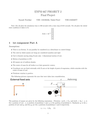
  • 1. ENPM 667 PROJECT 2 Final Project Suyash Yeotikar UID: 116188456, Nakul Patel UID:116334877 Note: For all plots the simulation time is 100 seconds with a time step of 0.01 seconds. For all plots the initial state condition is taken to be X(0) = 10−5         1 1 1 1 1 1         1 1st component Part A Assumptions: • There is no friction. It can possibly be considered as a disturbance in control design. • The rods by which masses are hung are considered massless and rigid • Cart is linearly moving along X-axis only. 1 dimensional motion of cart. • Motion of pendulum is 2-D. • All masses are of uniform density. • The center of mass for all bodies is at their geometric centers. • Coordinate axe are fixed externally with X axis at the height of point of suspension, which coincides with the center of mass of cart • Clockwise rotation is positive. The following pictures represents the axes that were taken into connsideration. The positions of masses are given by the following expressions. (Notation: cos θ1 = Cθ1 and sin θ1 = Sθ1 ). xc is the x position of cart. x1 is position of pendulum 1 and x2 is the position of pendulum 2. Similaryly yc is the y position of cart and y1 and the y2 are the y positions of pendulums 1 and 2 respectively. x1 = xc − l1Sθ1 (1) 1
  • 2. y1 = l1Cθ1 (2) x2 = xc − l2Sθ2 (3) y2 = l2Cθ2 (4) The velocities of masses in the respsective axes can be obtained by differentiating above expressions w.r.t time. ˙ x1 = ˙ xc − l1Cθ1 ˙ θ1 (5) ˙ y1 = −l1Sθ1 ˙ θ1 (6) ˙ x2 = ˙ xc − l2Cθ2 ˙ θ2 (7) ˙ y2 = −l2Sθ2 ˙ θ2 (8) From these the expression for kinetic energy of the whole system is , KE = 1 2 M ˙ xc 2 + 1 2 m1( ˙ xc − l1Cθ1 ˙ θ1)2 + 1 2 m1(−l1Sθ1 ˙ θ1)2 + 1 2 m2( ˙ xc − l2Cθ2 ˙ θ2)2 + 1 2 m2(−l2Sθ2 ˙ θ2)2 (9) Simplifying this we get, KE = 1 2 [M + m1 + m2] ˙ xc 2 + 1 2 m1l2 1 ˙ θ1 2 + 1 2 m2l2 2 ˙ θ2 2 − ˙ xc[m1l1Cθ1 ˙ θ1 + m2l2Cθ2 ˙ θ2] (10) The expression for potential energy is, PE = m1gl1Cθ1 + m2gl2Cθ2 (11) Writing the lagrangian from these, L = KE − PE (12) Partial Differentiating L w.r.t ˙ xc, ∂L ∂ ˙ xc = ˙ xc(M + m1 + m2) − (m1l1Cθ1 ˙ θ1 + m2l2Cθ2 ˙ θ2) (13) Differentiating lagrangian w.r.t xc, ∂L ∂xc = 0 Differentiating 13 w.r.t time, d dt ∂L ∂ ˙ xc = ¨ xc(M + m1 + m2) − m1l1(Cθ1 ¨ θ1 − Sθ1 ˙ θ1 2 ) − m2l2(Cθ2 ¨ θ2 − Sθ2 ˙ θ2 2 ) = F (14) Differentiating lagrangian w.r.t ˙ θ1 ∂L ∂ ˙ θ1 = − ˙ xcl1m1Cθ1 + m1l2 1 ˙ θ1 (15) d dt ∂L ∂ ˙ θ1 = m1l2 1 ¨ θ1 − m1l1( ¨ xcCθ1 − Sθ1 ˙ θ1 ˙ xc) (16) Differentiating largrangian w.r.t. θ1 ∂L ∂θ1 = m1l1gSθ1 + m1l1Sθ1 ˙ xc ˙ θ1 (17) Writing equation for ¨ θ1 m1l2 1 ¨ θ1 − m1l1( ¨ xcCθ1 − gSθ1 ) = 0 (18) Taking ¨ θ1 on one side, ¨ θ1 = ¨ xcCθ1 − gSθ1 l1 (19) 2
  • 3. Similarly for ¨ xc, ¨ xc = F + m1l1(Cθ1 ¨ θ1 − Sθ1 ˙ θ1 2 ) + m2l2(Cθ2 ¨ θ2 − Sθ2 ˙ θ2 2 ) M + m1 + m2 (20) Differentiating lagrangian w.r.t ˙ θ2 ∂L ∂ ˙ θ2 = − ˙ xcl2m2Cθ2 + m2l2 2 ˙ θ2 (21) d dt ∂L ∂ ˙ θ2 = m2l2 2 ¨ θ2 − m2l2( ¨ xcCθ2 − Sθ2 ˙ θ2 ˙ xc) (22) Differentiating largrangian w.r.t. θ2 ∂L ∂θ2 = m2l2gSθ2 + m2l2Sθ2 ˙ xc ˙ θ2 (23) Writing equation for ¨ θ2 m2l2 2 ¨ θ2 − m2l2( ¨ xcCθ2 − gSθ2 ) = 0 (24) Taking ¨ θ2 on one side, ¨ θ2 = ¨ xcCθ2 − gSθ2 l2 (25) Expressing all double differential terms only in 1st order and 0 order terms, Substituting equations 19 and 25, into equation 20, and simplifying we get., ¨ xc = F − 1 2 m1gS2∗θ1 − m1l1Sθ1 ˙ θ1 2 − 1 2 m2gS2∗θ2 − m2l2Sθ2 ˙ θ2 2 M + m1S2 θ1 + m2S2 θ2 (26) Substituting 25 in 20, ¨ xc = F + m1l1Cθ1 ¨ θ1 − m1l1Sθ1 ˙ θ1 2 − m2l2Sθ2 ˙ θ2 2 − m2gSθ2 Cθ2 M + m1 + m2S2 θ2 (27) Substituting 27 in 19, ¨ θ1 = [F − m1l1Sθ1 ˙ θ1 2 − m2l2Sθ2 ˙ θ2 2 − m2gSθ2 Cθ2 ]Cθ1 − [M + m1 + m2S2 θ2 ]gSθ1 l1[M + m1S2 θ1 + m2S2 θ2 ] (28) Substituting equation 19 in equation 20, ¨ xc = F + m2l2Cθ2 ¨ θ2 − m2l2Sθ2 ˙ θ2 2 − m1l1Sθ1 ˙ θ1 2 − m1gSθ1 Cθ1 M + m2 + m1S2 θ1 (29) Substiuting equation 29 in 25, ¨ θ2 = [F − m2l2Sθ2 ˙ θ2 2 − m1l1Sθ1 ˙ θ1 2 − m1gSθ1 Cθ1 ]Cθ2 − [M + m2 + m1S2 θ1 ]gSθ2 l2[M + m2S2 θ2 + m1S2 θ1 ] (29.1) writing above equations in non-linear state space form. Consider the following state vector, X =         ˙ xc ˙ θ1 ˙ θ2 xc θ1 θ2         =         x1 x2 x3 x4 x5 x6         (30) 3
  • 4. Ẋ =         ¨ xc ¨ θ1 ¨ θ2 ˙ xc ˙ θ1 ˙ θ2         (31) Ẋ =            F − 1 2 m1gS2x5 −m1l1Sx5 x2 2− 1 2 m2gS2x6 −m2l2Sx6 x2 3 M+m1S2 x5 +m2S2 x6 = [F −m1l1Sx5 x2 2−m2l2Sx6 x2 3−m2gSx6 Cx6 ]Cx5 −[M+m1+m2S2 x6 ]gSx5 l1[M+m1S2 x5 +m2S2 x6 ] [F −m1l1Sx5 x2 2−m2l2Sx6 x2 3−m1gSx5 Cx5 ]Cx6 −[M+m2+m1S2 x5 ]gSx6 l2[M+m1S2 x5 +m2S2 x6 ] x1 x2 x3            =         f1 f2 f3 f4 f5 f6         (31.1) And Y = CX Since there is a full state access in this paritcular case. where C =         1 0 0 0 0 0 0 1 0 0 0 0 0 0 1 0 0 0 0 0 0 1 0 0 0 0 0 0 1 0 0 0 0 0 0 1         (31.2) In the above equation, F is the input force, and the equations are written in terms of six states. 2 Part B Now, we linearize the above obtained non-linear system using jacobian linearization, around the equilibrium point, x = 0, θ1 = 0 and θ2 = 0. A system is said to be linearizable around an equilibrium point , if we can express the system in terms of linear matrices A, B, C, D , such that : AF = 5xF(x, u) (32) BF = 5uF(x, u) (33) CH = 5xH(x, u) (34) DH = 5uH(x, u) (35) where , the derivatives are calculated at equilibrium point. So, we can write the linearized A matrix as: Alin =          ∂f1 ∂x1 ∂f1 ∂x2 ∂f1 ∂x3 ∂f1 ∂x4 ∂f1 ∂x5 ∂f1 ∂x6 ∂f2 ∂x1 ∂f2 ∂x2 ∂f2 ∂x3 ∂f2 ∂x4 ∂f2 ∂x5 ∂f2 ∂x6 ∂f3 ∂x1 ∂f3 ∂x2 ∂f3 ∂x3 ∂f3 ∂x4 ∂f3 ∂x5 ∂f3 ∂x6 ∂f4 ∂x1 ∂f4 ∂x2 ∂f4 ∂x3 ∂f4 ∂x4 ∂f4 ∂x5 ∂f4 ∂x6 ∂f5 ∂x1 ∂f5 ∂x2 ∂f5 ∂x3 ∂f5 ∂x4 ∂f5 ∂x5 ∂f5 ∂x6 ∂f6 ∂x1 ∂f6 ∂x2 ∂f6 ∂x3 ∂f6 ∂x4 ∂f6 ∂x5 ∂f6 ∂x6          (36) 4
  • 5. Blin =                    ∂f1 ∂u ∂f2 ∂u ∂f3 ∂u ∂f4 ∂u ∂f5 ∂u ∂f6 ∂u                    (37) Finding the derivatives and evaluating them at equilibrium point , the following is obtined. (Refer code script linearimation.m). Alin =          0 0 0 0 −(gm1) M −(gm2) M 0 0 0 0 −(g(M+m1) Ml1 −(gm2) Ml1 0 0 0 0 −(gm1) Ml2 −g(M+m2) Ml2 1 0 0 0 0 0 0 1 0 0 0 0 0 0 1 0 0 0          (38) Blin =         1 M 1 Ml1 1 Ml2 0 0 0         (39) The. linearized state space representation will be, Ẋ = AlinX + BlinU (40) Y = CX (41) Where Alin and Blin are given by matrices in equations 38 and 39, and U = F and matrix C is given by, C =         1 0 0 0 0 0 0 1 0 0 0 0 0 0 1 0 0 0 0 0 0 1 0 0 0 0 0 0 1 0 0 0 0 0 0 1         (42) 3 Part C Refer linearimation.m script First it is checked if the system is controllable. Since the linearized system is a linear time invariant system, we use the rank condition for controllability matrix to check for the controllability. The controllability matrix in this case will be given by, controllability matrix = Blin AlinB A2 linB A3 linB A4 linB A5 linB (43) It is observed that the controllability matrix is a 6x6 matrix which. For a matrix to be full rank, it must have linearly independent row and column vectors. The linear independence can be tested by checking the determinant of the controllability matrix. If the determinant is not equal to zero, then the matrix will be full rank and thus controllable. So, first computing the determinant of controllability matrix, |controllability matrix| = −(g6 l2 1 − 2g6 l1l2 + g6 l2 2) (M6l6 1l6 2) (45) 5
  • 6. The above expression can be simplified as, |controllability matrix| = −g6 (l1 − l2)2 (M6l6 1l6 2) (46) For this expression to not be equal to 0 , l1 6= l2. Which is the condition for matrix to be full rank. Note that there is no dependency of condition on masses, and they can be anything, but if M is too high (powers of 10) then though the determinant might not actually be 0 but might go out of precision limits in certain frameworks and thus needs to be kept in mind. l1 6= l2 is the final condition. 4 Part D Substiuting the given values in Alin, and Blin, the following are obtained, Alin =         0 0 0 0 −0.9800 −0.9800 0 0 0 0 −0.5390 −0.0490 0 0 0 0 − 0.0980 −1.0780 1.0000 0 0 0 0 0 0 1.0000 0 0 0 0 0 0 1.0000 0 0 0         (47) Blin = 1.0e − 03         1.0000 0.0500 0.1000 0 0 0         (47.1) Substiuting these matrices in the controllability matrix the following controllability matrix was obtained, controllability matrix = 1.0e − 17 ∗         1.0000 0 0.0000 0 0.0000 0 0.0500 0 −0.0250 0 0.0125 0 0.1000 0 0.1000 0 0.1000 0 0 1.0000 0 0.0000 0 0.0000 0 0.0500 0 −0.0250 0 0.0125 0 0.1000 0 −0.1000 0 0.1000         (48) The rank of this matrix is found to be 6. Since, its a full rank matrix the system for substiuted values is controllable. To determine control input from the LQR controller, the matlab function ’lqr’ was used (Refer script). For different Q and R matrices different types of responses were obtained, as shown below. Q = 10         10 0 0 0 0 0 0 100 0 0 0 0 0 0 5 0 0 0 0 0 0 5 0 0 0 0 0 0 100 0 0 0 0 0 0 10         (49) R = 0.00001 (50) 6
  • 7. 7
  • 8. Q = 10         20 0 0 0 0 0 0 200 0 0 0 0 0 0 10 0 0 0 0 0 0 10 0 0 0 0 0 0 200 0 0 0 0 0 0 20         (51) R = 0.00002 (52) 8
  • 9. 9
  • 10. Q = 10         1 0 0 0 0 0 0 1 0 0 0 0 0 0 1 0 0 0 0 0 0 1 0 0 0 0 0 0 1 0 0 0 0 0 0 1         (53) R = 1 (54) 10
  • 11. 11
  • 12. Q =         10 5 80 2 6 10 10 20 100 50 20 10 30 50 30 10 10 10 20 60 10 30 20 40 30 10 10 10 20 80 60 10 20 60 50 10         (57) R = 0.001 (58) 12
  • 13. 13
  • 14. Observations and tuning: • It was observed that as Q and R were increased there were quite a lot of number of oscillations in the response of the system. This was expected since increasing Q and R would penalize heavily on the state change as well as the how much control input can be provided to the system. • In Q specifically if the state change of velocity cart was penalized more heavily then the response of the system significantly changed, more oscillations were induced. The oscillations mainly exist, and system requires significant control effort to converge because theere is huge amount of difference between the masses of cart and pendulums (almost 10 times), because of this discrepencies between the cost elements of Q matrix and lower R (cost on control input) is needed to have a faster convergence with fewr oscillations which is observed in figure 1. • If the other elements of the Q matrix apart from the diagonal matrix are changed then, the ’mutual’ state changes were observed to be penalized. This caused changes in the temporary characterstics of response of the system, in between oscillations. • The tuning for the system was done by observing the eigen values of the closed loop state Alin − BlinK matrix. By lyaponav’s indirect stability method the eigen values that matrix were in the left half plance, and the system is atleast locally stable. The 1st set of Q and R matrices (which is considered as a more suitable response) as shown. 5 Part E Refer script Luenberger Observer. For each of the output vectors given in the question, the corresponding C matrices will be will be. 14
  • 15. • x(t) C =         0 0 0 0 0 0 0 0 0 0 0 0 0 0 0 0 0 0 0 0 0 1 0 0 0 0 0 0 0 0 0 0 0 0 0 0         . (59) • (θ1(t), θ2(t)) C =         0 0 0 0 0 0 0 0 0 0 0 0 0 0 0 0 0 0 0 0 0 0 0 0 0 0 0 0 1 0 0 0 0 0 0 1         (60) • (x(t), θ2(t)) C =         0 0 0 0 0 0 0 0 0 0 0 0 0 0 0 0 0 0 0 0 0 1 0 0 0 0 0 0 0 0 0 0 0 0 0 1         (61) • (x(t), θ1(t)mθ2(t)) C =         0 0 0 0 0 0 0 0 0 0 0 0 0 0 0 0 0 0 0 0 0 1 0 0 0 0 0 0 1 0 0 0 0 0 0 1         (62) For each of these the Observability rank condition was checked for the linearized system. The observability matrix in this case for the linearized system will be given by will be given by, observability matrix =         C AlinC A2 linC A3 linC A4 linC A5 linC         (63) The rank for of obsvervability matrix for for x(t) was found to be 6, the rank of observability matrix for (θ1(t), θ2(t)) was found to be 4, the rank of observability matrix for (x(t), θ2(t) was found to be 6 and the rank of observability matrix for (x(t), θ1(t), θ2(t)) was found to be 6. The vectors for which observability matrix is full rank, will only be observable, hence the vectors x(t), (x(t), θ2(t)) and (x(t), θ1(t), θ2(t)) are observable. 6 Part F Step Function is defined as, U = ( 0 t 0 1 t ≥ 0 (64) Taking this as control input, and substituting it in the solution of the state space equation, and assuming that initial time is 0. X(t) = eAt X(0) + Z t 0 eAlin(t−τ) Blinu(τ)dτ (65) 15
  • 16. Subsituting u(τ) = 1, X(t) = eAt X(0) + Z t 0 eAlin(t−τ) Bdτ (66) X(t) = eAt X(0) + Z t 0 eAlint e−Aτ Bdτ (67) Taking eAlint and B out since they are not dependent on τ, X(t) = eAt X(0) + eAlint Z t 0 e−Aτ dτB (67.1) It is not possible to evaluate the integral further since Alin is not invertible (Determinant of Alin is 0). Hence the integral is evaluated as it is in MATLAB. Simulating with initial conditions, this gives the origian state vector. For an L matrix, then the errors at different time steps are obtained. The solution of error is not dependent on state vector. It is only dependent on initial error, A, L and C matrices. The solution of error is given by. ˙ e(t) = (A − LC)e (68) The above is obtained by subtracting Ẋ and ˙ X̂ Solving the above equation, error = e(A−LC)t error(0) (69) Here e(0) = X(0)− ˆ X(0) It is assumed that ˆ X(0) is a zero vector. Subtracting, X(t)−e(t) gives the state estimator. The ’best’ Luenberger observer is obtained by tuning L matrix. The tuning of L matrix is done by checking the eigenvalues of A − LC matrix. The eigen values must have high negative real part and low complex part for the luenberger observer to be best. For the non-linear system, instead of considering, error the the state estimator equation is directly considered. Consider the following State estimator equation, ˙ X̂ = f(X̂, U, t) + L(Y − Ŷ ) (70) This can be written as, ˙ X̂ = f(X̂, U, t) + LC(X − X̂) (71) since Y = CX and Ŷ = CX̂. To this the original non linear state equation is appended, and new set of equations is obtained, ˙ X̂ Ẋ # = f(X̂, U, t) + LC(X − X̂) f(X, U, t) (72) These set of 12 differential equations are given t the ODE45 solver in matlab which uses analytical Runge Kutta(reference) methods to solve for differential equations. The following are the plots of states vs. their estimates, for each of the L matrices corresponding to the output vectors for linear and non-linear systems. The figures have been shown only for 1st 10 seconds so as to observe the output and if X̂ and X are converging quickly or not. • For x(t) L =         30 12.5 8 11 0.2 0.08         16
  • 17. • For (x(t), θ2(t)) 17
  • 18. L =         12 12 0.55 0.55 12 12 10 10 0.75 0.75 0.05 0.05         18
  • 19. • For (x(t), θ1(t), θ1(t)) L =         10 10 10 0.5 0.5 0.5 10 10 10 6 6 6 1 1 1 0.01 0.01 0.01         19
  • 20. 7 Part G (Refer script LQG) Since the smallest observable output is just x(t), we design the LQG controller for the same. By seperation principle, it is possible to design the controller and observer separately. The controller has already been designed throught the LQR controller above. To design the observer Kalman filter function in MATLAB was used. The following values of Qn and Rn were used. Qn = 10 (73) Rn = 0.1 (74) We use the same frame work as above with the only difference that the L (Kalman Gain), will be computed using the Kalman filter. The following was the simulation obtained for the linear and non linear system. Here we use the same framework (code structure) as in previous part with the only difference that the L matrix (Kalman Gain) will be obtained from the Kalman Filter function. simulation upto 10 seconds 20
  • 21. simulation upto 100 seconds 21
  • 22. To get the system to track a constant reference error, a strategy similar to the that of lqr can be used. Let xd and u∞ be the desired states and the control input required to hold the state be known before hand.It is defined that, X̃ = X − Xd (75) X = X̃ + Xd (76) And, Ũ = U − U∞ (77) U = Ũ + U∞ (78) Substituing the above values in the state equation below, Ẋ = AlinX + BlinU + D (78.1) Then, ˙ X̃ + Xd = Alin(Xd + X̃) + Blin(Ũ + U∞) + D (79) Considering, AXd + BU∞ as the equilibrium point (equal to 0) and the reference does not change with time. ˙ X̃ = AlinX̃ + BlinŨ + D (80) The above process does not effect the error term in any way since the error term does not contiain X. ˙ error = (A − LC)error + D − LN (81) where N is measurement noise and D is the process noise. L is the kalman gain. The above frame work is similar to that of the standard LQG only with changed variable of X̃. The separation principle allows us to modify LQR and use a strategy similar to asymptotically track a constant reference in LQR and incorporate in the LQG system. In this case the solution would be given by, Ũ = −K ˆ X̃ (82) where, ˆ X̃ = X̂ − Xd (83) 22
  • 23. U = −K(X̂ − Xd) + U∞ (84) Note that, ˆ X̃ = X̃ + error (85) A simillar change of variable from X to X̃ in the non-linear system can be used, by replacing X with X +Xd. A con- stant disturbance would be a process noise which would have a covariance of 0. LQG does not solve for covariance of 0. Hence, LQG cannot solve for a constant disturbance. A possible work around for this could be by considering the process noise covariance to be significantly low 10− 5 . However, this results in large kalman gains. Following is the graph obtained in case of non-linear system when a constant disturbance of 10−3 1 1 1 1 1 1 although the system is seen to be stable it does not converge to the desired equilibrium point, there is a steady state error. It is like an offset. To overcome this an integral component of X̃ needs to be appended to the state so that steady state needs to be appended so that the steady state error is removed. However for the system to remain controllable we cannot append all states error, hence certain state errors need to prioritized l(maybe pendulums for crane) and ignore the cart steady state error. 23
  • 24. Run the scripts in following order: • llinearization.m • non linear sol.m • luenberger observed.m • non-linear luenberger.m • lqg.m 24
  • 25. 12/17/18 11:19 AM D:CONTROLS-PROJECT2linearization.m 1 of 4 %close all time_step = 0.01 sim_time = 100 syms M m1 m2 l1 l2 x1 x2 x3 x4 x5 x6 g syms F real syms M m1 m2 l1 l2 x1 x2 x3 x4 x5 x6 g real syms k1 k2 k3 k4 k5 k6 real %Representing the non-linear state-space equations f1 = (F - 0.5* m1*g*sin(2*x5) - m1*l1*sin(x5)*x2^2-0.5*m2*g*sin(2*x6)-m2*l2*sin(x6) *x3^2)/(M+m1*sin(x5)^2+m2*sin(x6)^2); f2 = ((F - m1*l1*sin(x5)*x2^2 - m2*l2*sin(x6)*x3^2 - m2*g*sin(x6)*cos(x6))*cos(x5) - (M+m1+m2*sin(x6)^2)*g*sin(x5))/(l1*(M+m1*sin(x5)^2+m2*sin(x6)^2)); f3 = ((F - m1*l1*sin(x5)*x2^2 - m2*l2*sin(x6)*x3^2 - m1*g*sin(x5)*cos(x5))*cos(x6) - (M+m2+m1*sin(x5)^2)*g*sin(x6))/(l2*(M+m1*sin(x5)^2+m2*sin(x6)^2)); f4 = x1; f5 = x2; f6 = x3; K = [ k1 ;k2; k3; k4; k5; k6]; %Linearizing the state-dynamics matrix A, B %Linearize the matrix A at the equilibrium point Jacob_A = [ diff(f1,x1) diff(f1,x2) diff(f1,x3) diff(f1,x4) diff(f1,x5) diff(f1,x6); diff(f2,x1) diff(f2,x2) diff(f2,x3) diff(f2,x4) diff(f2,x5) diff(f2,x6); diff(f3,x1) diff(f3,x2) diff(f3,x3) diff(f3,x4) diff(f3,x5) diff(f3,x6); diff(f4,x1) diff(f4,x2) diff(f4,x3) diff(f4,x4) diff(f4,x5) diff(f4,x6); diff(f5,x1) diff(f5,x2) diff(f5,x3) diff(f5,x4) diff(f5,x5) diff(f5,x6); diff(f6,x1) diff(f6,x2) diff(f6,x3) diff(f6,x4) diff(f6,x5) diff(f6,x6) ]; %Substituting the values of equilibrium point Jacob_A_sub=subs(Jacob_A, [x1 x2 x3 x4 x5 x6],[ 0 0 0 0 0 0]); D = M + m1*sin(x5)^2 + m2*sin(x6)^2; %Linearize the matrix B at the equilibrium point Jacob_B = [ diff(f1,F); diff(f2,F); diff(f3,F); diff(f4,F); diff(f5,F); diff(f6,F)]; %Substituting the values of equilibrium point Jacob_B_sub = subs(Jacob_B, [x1 x2 x3 x4 x5 x6],[ 0 0 0 0 0 0]); closed_loop = Jacob_B_sub*K' controllability_test = [ Jacob_B_sub Jacob_A_sub*Jacob_B_sub Jacob_A_sub^2*Jacob_B_sub Jacob_A_sub^3*Jacob_B_sub Jacob_A_sub^4*Jacob_B_sub Jacob_A_sub^5*Jacob_B_sub]; controllability_test_sub = double(subs(controllability_test,[l1 l2 M m1 m2 g],[20 10 1000 100 100 10])); check_rank = rank(controllability_test_sub) % A_lin1 = subs(Jacob_A, [l1 l2 M m1 m2 g],[20 10 1000 100 100 9.8]); A_lin = double(subs(A_lin1,[x1 x2 x3 x4 x5 x6],[0 0 0 0 0 0]));
  • 26. 12/17/18 11:19 AM D:CONTROLS-PROJECT2linearization.m 2 of 4 B_lin1 = subs(Jacob_B,[l1 l2 M m1 m2 g ],[20 10 1000 100 100 9.8]); B_lin = double(subs(B_lin1,[x1 x2 x3 x4 x5 x6],[0 0 0 0 0 0])); % Q_cost = 0.1*[1 5 5 5 5 5 % 5 1 5 5 5 5 % 5 5 1 5 5 5 % 5 5 5 1 5 5 % 5 5 5 5 1 5 % 5 5 5 5 5 1]; %Q_cost = 1000*eye(6,6); % Q_cost = 10*[10 3 2 5 2 3; % 3 100 5 2 2 3; % 2 4 5 2 2 4; % 5 7 6 5 6 6; % 2 5 2 5 100 6; % 3 7 3 5 4 10]; % R_cost = 0.0001; %Q1_R1 % Q_cost = 10*[20 0 0 0 0 0; % 0 100 0 0 0 0; % 0 0 10 0 0 0; % 0 0 0 10 0 0; % 0 0 0 0 100 0; % 0 0 0 0 0 20]; % % R_cost = 0.00002; %Q2_R2 % Q_cost = 10*[1 0 0 0 0 0; % 0 1 0 0 0 0; % 0 0 1 0 0 0; % 0 0 0 1 0 0; % 0 0 0 0 1 0; % 0 0 0 0 0 1]; % R_cost = 1; %Q3_R3 % Q_cost = 1*[0.5 0 0 0 0 0 ; % 0 0.5 0 0 0 0; % 0 0 0.5 0 0 0; % 0 0 0 0.5 0 0; % 0 0 0 0 0.5 0; % 0 0 0 0 0 0.5]; % R_cost = 0.5; %Q4_R4 %Defining the positive-definite weight matrices Q and R Q_cost = 10*[10 3 2 5 2 3; 3 100 5 2 2 3; 2 4 5 2 2 4; 5 7 6 5 6 6; 2 5 2 5 100 6;
  • 27. 12/17/18 11:19 AM D:CONTROLS-PROJECT2linearization.m 3 of 4 3 7 3 5 4 10]; R_cost = 0.0001; %Q5_R5 % Q_cost = 1*[10 5 80 2 6 10 ; % 10 20 100 50 20 10; % 30 50 30 10 10 10; % 20 60 10 30 20 40; % 30 10 10 10 20 80; % 60 10 20 60 50 10]; % R_cost = 0.001; %Designing the LQR controller, by defining the Q and R matrices above, %and giving A,B,Q,R as the parameters of lqr command. [K,s,e]= lqr(A_lin,B_lin,Q_cost,R_cost,0); syms t real x_init = 0.001*ones(6,1); x_fin=[]; test= A_lin-B_lin*K; eig(test) for t=0:time_step:sim_time x_fin_temp = expm((A_lin-B_lin*K).*t)*x_init; x_fin= [x_fin x_fin_temp]; end %figures for states-position, theta1 and theta2 figure title('States of the system') hold on plot([0:time_step:sim_time],x_fin(1,:),'b'); plot([0:time_step:sim_time],x_fin(2,:),'g'); plot([0:time_step:sim_time],x_fin(3,:),'r'); legend('Cart-position(linear)','Pendulum1(linear)','Pendulum2(linear)') % Defining the control input u=K*x_fin; figure hold on title('Control Input') plot(u,'b')
  • 28. 12/17/18 11:19 AM D:CONTROLS-PROJECT2linearization.m 4 of 4
  • 29. 12/17/18 11:19 AM D:CONTROLS-PROJECT2non_linear_sol.m 1 of 2 %Declaring the control input, for linear feedback control control_input = -K*[x1; x2; x3; x4; x5; x6]; f1_sub = simplify(vpa(subs(f1, [F l1 l2 M m1 m2 g],[ control_input 20 10 1000 100 100 9.8]))); f2_sub = simplify(vpa(subs(f2, [F l1 l2 M m1 m2 g],[ control_input 20 10 1000 100 100 9.8]))); f3_sub = simplify(vpa(subs(f3, [F l1 l2 M m1 m2 g],[ control_input 20 10 1000 100 100 9.8]))); %assuming that the oscillations are really small. %f1_sub1 = subs(f1_sub,[sin(x5) cos(x5) sin(x6) cos(x6)],[ x5 1 x6 1]); %f2_sub1 = subs(f2_sub,[sin(x5) cos(x5) sin(x6) cos(x6)],[ x5 1 x6 1]); %f3_sub1 = subs(f3_sub,[sin(x5) cos(x5) sin(x6) cos(x6)],[ x5 1 x6 1]); syms x1t(t) x2t(t) x3t(t) x4t(t) x5t(t) x6t(t) real f1_sub1_t = subs(f1_sub,[ x1 x2 x3 x4 x5 x6],[x1t x2t x3t x4t x5t x6t]); f2_sub1_t = subs(f2_sub,[ x1 x2 x3 x4 x5 x6],[x1t x2t x3t x4t x5t x6t]); f3_sub1_t = subs(f3_sub,[ x1 x2 x3 x4 x5 x6],[x1t x2t x3t x4t x5t x6t]); state_vec = [x1t; x2t; x3t; x4t; x5t; x6t]; diff_eqn1 = diff(x1t,t,1)== f1_sub1_t; diff_eqn2 = diff(x2t,t,1)== f2_sub1_t; diff_eqn3 = diff(x3t,t,1) == f3_sub1_t; diff_eqn4= diff(x4t,t,1) == x1t; diff_eqn5 = diff(x5t,t,1) == x2t; diff_eqn6 = diff(x6t,t,1) == x3t; eqns = [ diff_eqn1; diff_eqn2; diff_eqn3; diff_eqn4; diff_eqn5; diff_eqn6]; [M1,F1] = massMatrixForm(eqns,state_vec); f = M1F1; ode_fun = odeFunction(f,state_vec); [t,x_out] = ode45(ode_fun,[0 sim_time],x_init); figure; hold on; title('States for non-linear system') plot(t,x_out(:,1)); plot(t,x_out(:,2)); plot(t,x_out(:,3)); legend('Cart-position(non-linear)','Pendulum1(non-linear)','Pendulum2(non-linear)') % % For the phase-plots(position) % hold on % title('Phase-plot for position and velocity') % xout_t=x_out'; % plot(xout_t(1,:),xout_t(4,:),'b'); % % % For the phase-plot(theta1) % figure % hold on % title('Phase-plot for theta1 and theta1dot') % xout_t=x_out';
  • 30. 12/17/18 11:19 AM D:CONTROLS-PROJECT2non_linear_sol.m 2 of 2 % plot(xout_t(2,:),xout_t(5,:),'b'); % % % For the phase-plot(theta2) % figure % hold on % title('Phase-plot for theta2 and theta2dot') % xout_t=x_out'; % plot(xout_t(3,:),xout_t(6,:),'b');
  • 31. 12/17/18 11:19 AM D:CONTROLS-P...Leunberger_observer.m 1 of 4 %Second Part--Observability close all sim_time=10; %Declaration of C matrices/vector for corresponding output vectors Cx=[0 0 0 1 0 0] %----observable; Ct1t2=[0 0 0 0 0 0;0 0 0 0 0 0;0 0 0 0 0 0;0 0 0 0 0 0;0 0 0 0 1 0;0 0 0 0 0 1]; Cxt2=[0 0 0 1 0 0;0 0 0 0 0 1] %----observable; Cxt1t2=[0 0 0 1 0 0;0 0 0 0 1 0;0 0 0 0 0 1] %----observable; %Checking the condition for observability O1=rank([Cx; Cx*A_lin; Cx*A_lin^2; Cx*A_lin^3; Cx*A_lin^4; Cx*A_lin^5]); O2=rank([Ct1t2; Ct1t2*A_lin; Ct1t2*A_lin^2; Ct1t2*A_lin^3; Ct1t2*A_lin^4; Ct1t2*A_lin^5]); O3=rank([Cxt2; Cxt2*A_lin; Cxt2*A_lin^2; Cxt2*A_lin^3; Cxt2*A_lin^4; Cxt2*A_lin^5]); O4=rank([Cxt1t2; Cxt1t2*A_lin; Cxt1t2*A_lin^2; Cxt1t2*A_lin^3; Cxt1t2*A_lin^4; Cxt1t2*A_lin^5]); %Step input(for simulation) x_fin2=[]; syms tau integral=vpa(int(expm(-A_lin).*tau)); for t=0:time_step:sim_time x_fin_temp3 = expm((A_lin).*t)*x_init + expm((A_lin).*t)*subs(integral,tau ,t) *B_lin ; x_fin2= [x_fin2 x_fin_temp3]; t end figure hold on title('') plot([0:time_step:sim_time],x_fin2(1,:),'b'); plot([0:time_step:sim_time],x_fin2(2,:),'g'); plot([0:time_step:sim_time],x_fin2(3,:),'r'); %Leunberger Observer %For the first controllability matrix(first vector of output) x_error=x_init; L=[ 30; 12.5; 8 ; 11; 0.2 ; 0.08]; % L=[ 30; % 0.7;
  • 32. 12/17/18 11:19 AM D:CONTROLS-P...Leunberger_observer.m 2 of 4 % 10 ; % 6; % 1 ; % 0.01]; x_error_dot=(A_lin-L*Cx)*x_error; % Solution for first output vector x_fin3=[]; for t=0:time_step:sim_time x_fin_temp = expm((A_lin-L*Cx).*t)*x_error; x_fin3= [x_fin3 x_fin_temp]; end figure title('For First output vector(Linear)') hold on plot([0:time_step:sim_time],x_fin2(1,:)-x_fin3(1,:),'--','Color',[1,0,0]); plot([0:time_step:sim_time],x_fin2(1,:),'r'); plot([0:time_step:sim_time],x_fin2(2,:)-x_fin3(2,:),'--','Color',[0,1,0]); plot([0:time_step:sim_time],x_fin2(2,:),'g'); plot([0:time_step:sim_time],x_fin2(3,:)-x_fin3(3,:),'--','Color',[0,0,1]); plot([0:time_step:sim_time],x_fin2(3,:),'b'); legend('xchat','xc','t1hat','t1','t2hat','t2') %plot([0:time_step:sim_time],x_fin2(3,:)-x_fin3(3,:),'r'); eig(A_lin-L*Cx) % For the third controllability matrix(third vector of output) L_3=[ 12 12; 0.55 0.55; 12 12; 10 10; 0.75 0.75; 0.05 0.05]; % L_3=[ 7.5 7.5; % 0.3 0.3; % 8 8; % 6 6; % 1 1; % 0.2 0.2]; x_error_dot3=(A_lin-L_3*Cxt2)*x_error;
  • 33. 12/17/18 11:19 AM D:CONTROLS-P...Leunberger_observer.m 3 of 4 % Solution for third output vector x_fin4=[]; for t=0:time_step:sim_time x_fin_temp = expm((A_lin-L_3*Cxt2).*t)*x_error; x_fin4= [x_fin4 x_fin_temp]; end figure title('For Third output vector(Linear)') hold on plot([0:time_step:sim_time],x_fin2(1,:)-x_fin4(1,:),'--','Color',[1,0,0]); plot([0:time_step:sim_time],x_fin2(1,:),'r'); plot([0:time_step:sim_time],x_fin2(2,:)-x_fin4(1,:),'--','Color',[0,1,0]); plot([0:time_step:sim_time],x_fin2(2,:),'g'); plot([0:time_step:sim_time],x_fin2(3,:)-x_fin4(1,:),'--','Color',[0,0,1]); plot([0:time_step:sim_time],x_fin2(3,:),'b'); legend('xchat','xc','t1hat','t1','t2hat','t2') %plot([0:time_step:sim_time],x_fin2(3,:)-x_fin3(3,:),'r'); eig(A_lin-L_3*Cxt2) % For the fourth controllability matrix(fourth vector of output) L_4=[ 10 10 10; 0.5 0.5 0.5; 10 10 10; 6 6 6; 1 1 1; 0.01 0.01 0.01]; x_error_dot4=(A_lin-L_4*Cxt1t2)*x_error; % Solution for fourth output vector x_fin5=[]; for t=0:time_step:sim_time x_fin_temp = expm((A_lin-L_4*Cxt1t2).*t)*x_error; x_fin5= [x_fin5 x_fin_temp]; end figure title('For Fourth output vector(Linear)') hold on plot([0:time_step:sim_time],x_fin2(1,:)-x_fin5(1,:),'--','Color',[1,0,0]);
  • 34. 12/17/18 11:19 AM D:CONTROLS-P...Leunberger_observer.m 4 of 4 plot([0:time_step:sim_time],x_fin2(1,:),'r'); plot([0:time_step:sim_time],x_fin2(2,:)-x_fin5(1,:),'--','Color',[0,1,0]); plot([0:time_step:sim_time],x_fin2(2,:),'g'); plot([0:time_step:sim_time],x_fin2(3,:)-x_fin5(1,:),'--','Color',[0,0,1]); plot([0:time_step:sim_time],x_fin2(3,:),'b'); legend('xchat','xc','t1hat','t1','t2hat','t2') %plot([0:time_step:sim_time],x_fin2(3,:)-x_fin3(3,:),'r'); eig(A_lin-L_4*Cxt1t2) %L=[0 0 0 10 0 0; % 0 0 0 0.5 0 0; % 0 0 0 10 0 0; % 0 0 0 5 0 0; % 0 0 0 1 0 0; % 0 0 0 0.01 0 0]; %L_3=[0 0 0 10 0 10; % 0 0 0 0.5 0 0.5; % 0 0 0 10 0 10; % 0 0 0 5 0 5; % 0 0 0 1 0 1; % 0 0 0 0.01 0 0.01]; %L_4=[0 0 0 10 10 10; % 0 0 0 0.5 0.5 0.5; % 0 0 0 10 10 10; % 0 0 0 5 5 5; % 0 0 0 1 1 1; % 0 0 0 0.01 0.01 0.01];
  • 35. 12/17/18 11:20 AM D:CONTROLS...non_linear_luenberger.m 1 of 3 %Implementing the Luenberger observer for non-linear system control_input2 = 1; f1_sub2 = simplify(vpa(subs(f1, [F l1 l2 M m1 m2 g],[ 1 20 10 1000 100 100 9.8])),5); f2_sub2 = simplify(vpa(subs(f2, [F l1 l2 M m1 m2 g],[ 1 20 10 1000 100 100 9.8])),5); f3_sub2 = simplify(vpa(subs(f3, [F l1 l2 M m1 m2 g],[ 1 20 10 1000 100 100 9.8])),5); f1_sub2_t = subs(f1_sub2,[ x1 x2 x3 x4 x5 x6],[x1t x2t x3t x4t x5t x6t]); f2_sub2_t = subs(f2_sub2,[ x1 x2 x3 x4 x5 x6],[x1t x2t x3t x4t x5t x6t]); f3_sub2_t = subs(f3_sub2,[ x1 x2 x3 x4 x5 x6],[x1t x2t x3t x4t x5t x6t]); syms x1hat(t) x2hat(t) x3hat(t) x4hat(t) x5hat(t) x6hat(t) real f1_sub2_hat = subs(f1_sub2,[ x1 x2 x3 x4 x5 x6],[x1hat x2hat x3hat x4hat x5hat x6hat]); f2_sub2_hat = subs(f2_sub2,[ x1 x2 x3 x4 x5 x6],[x1hat x2hat x3hat x4hat x5hat x6hat]); f3_sub2_hat = subs(f3_sub2,[ x1 x2 x3 x4 x5 x6],[x1hat x2hat x3hat x4hat x5hat x6hat]); LnC = L*Cx; vec_xt= [ x1t; x2t; x3t; x4t;x5t;x6t]; vec_xhat =[ x1hat; x2hat; x3hat; x4hat; x5hat; x6hat]; diff_eqn1 = diff(x1hat,t,1)==f1_sub2_hat+ LnC(1,:)*(vec_xt-vec_xhat); diff_eqn2 = diff(x2hat,t,1)==f2_sub2_hat+ LnC(2,:)*(vec_xt-vec_xhat); diff_eqn3 = diff(x3hat,t,1)==f3_sub2_hat+ LnC(3,:)*(vec_xt-vec_xhat); diff_eqn4= diff(x4hat,t,1)==x1hat + LnC(4,:)*(vec_xt-vec_xhat); diff_eqn5 = diff(x5hat,t,1)==x2hat + LnC(5,:)*(vec_xt-vec_xhat); diff_eqn6 = diff(x6hat,t,1)==x3hat + LnC(6,:)*(vec_xt-vec_xhat); diff_eqn7 = diff(x1t,t,1)== f1_sub2_t; diff_eqn8 = diff(x2t,t,1)== f2_sub2_t; diff_eqn9 = diff(x3t,t,1) == f3_sub2_t; diff_eqn10= diff(x4t,t,1) == x1t; diff_eqn11 = diff(x5t,t,1) == x2t; diff_eqn12 = diff(x6t,t,1) == x3t; state_vec1= [vec_xhat; vec_xt]; eqns2 = [ diff_eqn1; diff_eqn2; diff_eqn3; diff_eqn4; diff_eqn5; diff_eqn6; diff_eqn7; diff_eqn8; diff_eqn9; diff_eqn10; diff_eqn11;diff_eqn12]; [M3,F3] = massMatrixForm(eqns2,state_vec1); f = M3F3; ode_fun = odeFunction(f,state_vec1); x_init2 =[zeros(6,1); x_init]; [t,x_out] = ode45(ode_fun,[0 sim_time],x_init2); figure; title('For First output vector(non-linear)') hold on; plot(t,x_out(:,10),'r'); plot(t,x_out(:,4),'--','Color',[1,0,0]); plot(t,x_out(:,11),'g'); plot(t,x_out(:,5),'--','Color',[0,1,0]); plot(t,x_out(:,12),'b'); plot(t,x_out(:,6),'--','Color',[0,0,1]); legend('xc','xchat','t1','t1hat','t2','t2hat')
  • 36. 12/17/18 11:20 AM D:CONTROLS...non_linear_luenberger.m 2 of 3 %plot(t,x_out(:,12),'r'); % (For third output Vector) syms x1hat(t) x2hat(t) x3hat(t) x4hat(t) x5hat(t) x6hat(t) real LnC_3 = L_3*Cxt2; diff_eqn1 = diff(x1hat,t,1)==f1_sub2_hat+ LnC_3(1,:)*(vec_xt-vec_xhat); diff_eqn2 = diff(x2hat,t,1)==f2_sub2_hat+ LnC_3(2,:)*(vec_xt-vec_xhat); diff_eqn3 = diff(x3hat,t,1)==f3_sub2_hat+ LnC_3(3,:)*(vec_xt-vec_xhat); diff_eqn4= diff(x4hat,t,1)==x1hat + LnC_3(4,:)*(vec_xt-vec_xhat); diff_eqn5 = diff(x5hat,t,1)==x2hat + LnC_3(5,:)*(vec_xt-vec_xhat); diff_eqn6 = diff(x6hat,t,1)==x3hat + LnC_3(6,:)*(vec_xt-vec_xhat); diff_eqn7 = diff(x1t,t,1)== f1_sub2_t; diff_eqn8 = diff(x2t,t,1)== f2_sub2_t; diff_eqn9 = diff(x3t,t,1) == f3_sub2_t; diff_eqn10= diff(x4t,t,1) == x1t; diff_eqn11 = diff(x5t,t,1) == x2t; diff_eqn12 = diff(x6t,t,1) == x3t; eqns2 = [ diff_eqn1; diff_eqn2; diff_eqn3; diff_eqn4; diff_eqn5; diff_eqn6; diff_eqn7; diff_eqn8; diff_eqn9; diff_eqn10; diff_eqn11;diff_eqn12]; [M3,F3] = massMatrixForm(eqns2,state_vec1); f = M3F3; ode_fun = odeFunction(f,state_vec1); x_init3 =[zeros(6,1); x_init]; [t,x_out] = ode45(ode_fun,[0 sim_time],x_init3); figure; title('For Third output vector(non-linear)') hold on; plot(t,x_out(:,10),'r'); plot(t,x_out(:,4),'--','Color',[1,0,0]); plot(t,x_out(:,11),'g'); plot(t,x_out(:,5),'--','Color',[0,1,0]); plot(t,x_out(:,12),'b'); plot(t,x_out(:,6),'--','Color',[0,0,1]); legend('xc','xchat','t1','t1hat','t2','t2hat') %plot(t,x_out(:,12),'r'); % (For fourth output Vector) syms x1hat(t) x2hat(t) x3hat(t) x4hat(t) x5hat(t) x6hat(t) real LnC_4 = L_4*Cxt1t2; diff_eqn1 = diff(x1hat,t,1)==f1_sub2_hat+ LnC_4(1,:)*(vec_xt-vec_xhat); diff_eqn2 = diff(x2hat,t,1)==f2_sub2_hat+ LnC_4(2,:)*(vec_xt-vec_xhat); diff_eqn3 = diff(x3hat,t,1)==f3_sub2_hat+ LnC_4(3,:)*(vec_xt-vec_xhat);
  • 37. 12/17/18 11:20 AM D:CONTROLS...non_linear_luenberger.m 3 of 3 diff_eqn4= diff(x4hat,t,1)==x1hat + LnC_4(4,:)*(vec_xt-vec_xhat); diff_eqn5 = diff(x5hat,t,1)==x2hat + LnC_4(5,:)*(vec_xt-vec_xhat); diff_eqn6 = diff(x6hat,t,1)==x3hat + LnC_4(6,:)*(vec_xt-vec_xhat); diff_eqn7 = diff(x1t,t,1)== f1_sub2_t; diff_eqn8 = diff(x2t,t,1)== f2_sub2_t; diff_eqn9 = diff(x3t,t,1) == f3_sub2_t; diff_eqn10= diff(x4t,t,1) == x1t; diff_eqn11 = diff(x5t,t,1) == x2t; diff_eqn12 = diff(x6t,t,1) == x3t; eqns2 = [ diff_eqn1; diff_eqn2; diff_eqn3; diff_eqn4; diff_eqn5; diff_eqn6; diff_eqn7; diff_eqn8; diff_eqn9; diff_eqn10; diff_eqn11;diff_eqn12]; [M3,F3] = massMatrixForm(eqns2,state_vec1); f = M3F3; ode_fun = odeFunction(f,state_vec1); x_init4 =[zeros(6,1); x_init]; [t,x_out] = ode45(ode_fun,[0 sim_time],x_init4); figure; title('For Fourth output vector(non-linear)') hold on; plot(t,x_out(:,10),'r'); plot(t,x_out(:,4),'--','Color',[1,0,0]); plot(t,x_out(:,11),'g'); plot(t,x_out(:,5),'--','Color',[0,1,0]); plot(t,x_out(:,12),'b'); plot(t,x_out(:,6),'--','Color',[0,0,1]); legend('xc','xchat','t1','t1hat','t2','t2hat') %plot(t,x_out(:,12),'r');
  • 38. 12/17/18 11:20 AM D:CONTROLS-PROJECT2lqg.m 1 of 2 sys1 = ss(A_lin,[B_lin ones(6,1)],Cx,0); %converting into state space Qn = (10); % setting covraince matrices Rn = (0.000001); [kest,L_kal] = kalman(sys1,Qn,Rn,0); %using kalman filter to estimate kalman gain reg = lqgreg(kest, K); syms x1t(t) x2t(t) x3t(t) x4t(t) x5t(t) x6t(t) syms x1hat(t) x2hat(t) x3hat(t) x4hat(t) x5hat(t) x6hat(t); disturbance_vec = [0.001 0.001 0.001 0.001 0.001 0.001]'; % reference and control_input3= vpa(-K*(vec_xhat)); % setting control input from LQR %solving for non linear model by appending states with hat and using ode45 %to solve. f1_sub4 = simplify(vpa(subs(f1, [F l1 l2 M m1 m2 g],[ control_input3 20 10 1000 100 100 9.8]))); f2_sub4 = simplify(vpa(subs(f2, [F l1 l2 M m1 m2 g],[ control_input3 20 10 1000 100 100 9.8]))); f3_sub4 = simplify(vpa(subs(f3, [F l1 l2 M m1 m2 g],[ control_input3 20 10 1000 100 100 9.8]))); f1_sub4_t = subs(f1_sub4,[ x1 x2 x3 x4 x5 x6],[x1t x2t x3t x4t x5t x6t]); f2_sub4_t = subs(f2_sub4,[ x1 x2 x3 x4 x5 x6],[x1t x2t x3t x4t x5t x6t]); f3_sub4_t = subs(f3_sub4,[ x1 x2 x3 x4 x5 x6],[x1t x2t x3t x4t x5t x6t]); f1_sub4_hat = subs(f1_sub4,[ x1 x2 x3 x4 x5 x6],[x1hat x2hat x3hat x4hat x5hat x6hat]); f2_sub4_hat = subs(f2_sub4,[ x1 x2 x3 x4 x5 x6],[x1hat x2hat x3hat x4hat x5hat x6hat]); f3_sub4_hat = subs(f3_sub4,[ x1 x2 x3 x4 x5 x6],[x1hat x2hat x3hat x4hat x5hat x6hat]); LnC_kal = L_kal*Cx; diff_eqn11 = diff(x1hat,t,1)==f1_sub4_hat+ LnC_kal(1,:)*(vec_xt-vec_xhat) +disturbance_vec(1,1); diff_eqn21 = diff(x2hat,t,1)==f2_sub4_hat+ LnC_kal(2,:)*(vec_xt-vec_xhat) +disturbance_vec(2,1); diff_eqn31 = diff(x3hat,t,1)==f3_sub4_hat+ LnC_kal(3,:)*(vec_xt-vec_xhat) +disturbance_vec(3,1); diff_eqn41= diff(x4hat,t,1)==x1hat + LnC_kal(4,:)*(vec_xt-vec_xhat)+disturbance_vec (4,1); diff_eqn51 = diff(x5hat,t,1)==x2hat + LnC_kal(5,:)*(vec_xt-vec_xhat)+disturbance_vec (5,1); diff_eqn61 = diff(x6hat,t,1)==x3hat+ LnC_kal(6,:)*(vec_xt-vec_xhat)+disturbance_vec (6,1); diff_eqn71 = diff(x1t,t,1)== f1_sub4_t + disturbance_vec(1,1); diff_eqn81 = diff(x2t,t,1)== f2_sub4_t+ disturbance_vec(2,1); diff_eqn91 = diff(x3t,t,1) == f3_sub4_t+disturbance_vec(3,1); diff_eqn101= diff(x4t,t,1) == x1t+disturbance_vec(4,1); diff_eqn111 = diff(x5t,t,1) == x2t+disturbance_vec(5,1); diff_eqn121 = diff(x6t,t,1) == x3t+disturbance_vec(6,1); state_vec1= [vec_xhat; vec_xt]; eqns3 = [ diff_eqn11; diff_eqn21; diff_eqn31; diff_eqn41; diff_eqn51; diff_eqn61; diff_eqn71; diff_eqn81; diff_eqn91; diff_eqn101; diff_eqn111;diff_eqn121];
  • 39. 12/17/18 11:20 AM D:CONTROLS-PROJECT2lqg.m 2 of 2 [M4,F4] = massMatrixForm(eqns3,state_vec1); f = M4F4; ode_fun2 = odeFunction(f,state_vec1); x_init2 =[zeros(6,1); x_init]; [t,x_out3] = ode45(ode_fun2,[0 sim_time],x_init2); figure; hold on; %plots plot(t,x_out3(:,10),'r'); plot(t,x_out3(:,4),'--','Color',[1,0,0]); plot(t,x_out3(:,11),'g'); plot(t,x_out3(:,5),'--','Color',[0,1,0]); plot(t,x_out3(:,12),'b'); plot(t,x_out3(:,6),'--','Color',[0,0,1]); legend('xc','xchat','t1','t1hat','t2','t2hat') %eig(A_lin-L_kal*Cx) % eigen value check of error figure; hold on; plot(t,x_out3(:,7),'r'); plot(t,x_out3(:,1),'--','Color',[1,0,0]); plot(t,x_out3(:,8),'g'); plot(t,x_out3(:,2),'--','Color',[0,1,0]); plot(t,x_out3(:,9),'b'); plot(t,x_out3(:,3),'--','Color',[0,0,1]); legend('xcdot','xchatdot','t1dot','t1hatdot','t2dot','t2hatdot')