Data Science Using Python notes

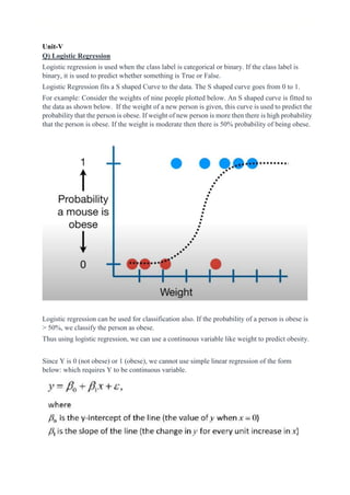
1. Unit-V
Q) Logistic Regression
Logistic regression is used when the class label is categorical or binary. If the class label is
binary, it is used to predict whether something is True or False.
Logistic Regression fits a S shaped Curve to the data. The S shaped curve goes from 0 to 1.
For example: Consider the weights of nine people plotted below. An S shaped curve is fitted to
the data as shown below. If the weight of a new person is given, this curve is used to predict the
probability that the person is obese. If weight of new person is more then there is high probability
that the person is obese. If the weight is moderate then there is 50% probability of being obese.
Logistic regression can be used for classification also. If the probability of a person is obese is
> 50%, we classify the person as obese.
Thus using logistic regression, we can use a continuous variable like weight to predict obesity.
Since Y is 0 (not obese) or 1 (obese), we cannot use simple linear regression of the form
below: which requires Y to be continuous variable.

2. https://www.youtube.com/watch?v=yIYKR4sgzI8
https://www.youtube.com/watch?v=vN5cNN2-
HWE&list=PLblh5JKOoLUICTaGLRoHQDuF_7q2GfuJF&index=17
https://slidetodoc.com/introduction-to-regression-model-xueying-li-ms-senior/
Q) Bottom up Hierarchical Clustering
Ans: Hierarchical clustering is another unsupervised machine learning algorithm, which is used
to group the unlabeled datasets into a cluster. It is also known as hierarchical cluster analysis or
HCA.
In this algorithm, we develop the hierarchy of clusters in the form of a tree, and this tree-shaped
structure is known as the dendrogram.
The hierarchical clustering technique has two approaches:
1. Agglomerative: Agglomerative is a bottom-up approach, in which the algorithm starts
with taking all data points as single clusters and merging them until one cluster is left.

3. 2. Divisive: Divisive algorithm is the reverse of the agglomerative algorithm as it is a top-
down approach.
Agglomerative Hierarchical clustering
The agglomerative hierarchical clustering algorithm is a popular example of HCA. To group
the datasets into clusters, it follows the bottom-up approach. It means, this algorithm
considers each dataset as a single cluster at the beginning, and then start combining the closest
pair of clusters together. It does this until all the clusters are merged into a single cluster that
contains all the datasets.
This hierarchy of clusters is represented in the form of the dendrogram.
Here's an overview of the steps involved in bottom-up hierarchical clustering:
Step 1: Initialise each data point as its own cluster: We start by treating each data point as its
own cluster.
Step 2: Calculate the distance between each pair of clusters: There are different ways to calculate
the distance, such as Euclidean distance, Manhattan distance, and cosine similarity.
Step 3: Merge the two closest clusters: We then calculate the distance between each pair of
clusters and merge the two closest clusters into a single cluster. The distance between clusters
can be calculated using single linkage, complete linkage, or average linkage, which are different
ways of measuring the distance between clusters.
Step 4: Update the distance matrix: After merging two clusters, we need to update the distance
matrix to reflect the new distances between clusters. This involves calculating the distance
between the new merged cluster and each of the remaining clusters.

4. Repeat steps 3 and 4 until a stopping criterion is met: We repeat steps 3 and 4 until all of the data
points are in a single cluster or until a stopping criterion is met. The stopping criterion can be
based on the number of clusters, the distance between clusters, or other factors.
How the Agglomerative Hierarchical clustering Work?
The working of the AHC algorithm can be explained using the below steps:
● Step-1: Create each data point as a single cluster. Let's say there are N data points, so
the number of clusters will also be N.
● Step-2: Take two closest data points or clusters and merge them to form one cluster.
So, there will now be N-1 clusters.

5. ● Step-3: Again, take the two closest clusters and merge them together to form one
cluster. There will be N-2 clusters.
● Step-4: Repeat Step 3 until only one cluster left. So, we will get the following clusters.
Consider the below images:
● Step-5: Once all the clusters are combined into one big cluster, develop the dendrogram
to divide the clusters as per the problem.
Measure for the distance between two clusters
As we have seen, the closest distance between the two clusters is crucial for the hierarchical
clustering. There are various ways to calculate the distance between two clusters, and these

6. ways decide the rule for clustering. These measures are called Linkage methods. Some of the
popular linkage methods are given below:
1. Single Linkage: It is the Shortest Distance between the closest points of the clusters.
Single linkage tends to produce long, chain-like clusters. Consider the below image:
2. Complete Linkage: It is the farthest distance between the two points of two different
clusters. It is one of the popular linkage methods as it forms tighter clusters than single-
linkage. Complete linkage tends to produce compact, spherical clusters.
3. Average Linkage: It is the linkage method in which the distance between each pair of
datasets is added up and then divided by the total number of datasets to calculate the

7. average distance between two clusters. It is also one of the most popular linkage
methods.
4. Centroid Linkage: It is the linkage method in which the distance between the centroid
of the clusters is calculated. Centroid linkage can be useful for high-dimensional data
where the distance between individual points may be less meaningful. Consider the
below image:
From the above-given approaches, we can apply any of them according to the type of problem
or business requirement.
Woking of Dendrogram in Hierarchical clustering
The dendrogram is a tree-like structure that is mainly used to store each step as a memory that
the HC algorithm performs. In the dendrogram plot, the Y-axis shows the Euclidean distances
between the data points, and the x-axis shows all the data points of the given dataset.
The working of the dendrogram can be explained using the below diagram:

8. In the above diagram, the left part is showing how clusters are created in agglomerative
clustering, and the right part is showing the corresponding dendrogram.
● As we have discussed above, firstly, the data points P2 and P3 combine together and
form a cluster, correspondingly a dendrogram is created, which connects P2 and P3
with a rectangular shape. The height is decided according to the Euclidean distance
between the data points.
● In the next step, P5 and P6 form a cluster, and the corresponding dendrogram is created.
It is higher than the previous, as the Euclidean distance between P5 and P6 is a little bit
greater than the P2 and P3.
● Again, two new dendrograms are created that combine P1, P2, and P3 in one
dendrogram, and P4, P5, and P6, in another dendrogram.
● At last, the final dendrogram is created that combines all the data points together.
We can cut the dendrogram tree structure at any level as per our requirement.
Q) Multiple Linear Regression
Multiple regression is an extension of linear regression.
It finds relationships between more than two variables. In simple linear relation we have one
independent and one dependent variable, but in multiple regression we have more than one
independent variable and one dependent variable.
Examples:

9. The general mathematical equation for multiple regression is −
y = a1x1+a2x2+...+b
Following is the description of the parameters used −
y is the response variable.
b, a1, a2...an are the coefficients.
x1, x2, ...xn are the predictor variables.
Model fitting: The coefficients b,a1,a2 are estimated using a method such as least squares or
maximum likelihood estimation.
These methods minimise the sum of squared residuals/errors between the predicted and actual
values.
Model assumptions: Multiple regression assumes linearity, independence, homoscedasticity,
and normality of errors. Linearity means that the relationship between the independent and
dependent variables is linear. Independence means that the observations are independent of
each other. Homoscedasticity means that the variance of the errors is constant across all levels
of the independent variables. Normality of errors means that the errors are normally distributed.
Model evaluation: Multiple regression models can be evaluated based on their goodness of fit.
Goodness of fit is measured by R-squared and adjusted R-squared values. R-squared represents
the proportion of variation in the dependent variable that is explained by the independent
variables. The adjusted R-squared adjust R-squared for the number of independent variables in
the model.

10. Model interpretation: The coefficients of the independent variables represent the change in the
dependent variable for a unit change in the independent variable. All other independent
variables are constant. The p-value of each coefficient tests the hypothesis that the coefficient
is equal to zero, and a low p-value indicates that the coefficient is significantly different from
zero.
Model limitations: Multiple regression is limited by its assumptions, and violating these
assumptions can lead to incorrect results. Additionally, multiple regression can be prone to
overfitting, where the model fits the noise in the data rather than the underlying relationship.
In summary, multiple regression is a powerful tool for understanding the relationship between
multiple independent variables and a dependent variable. However, it is important to carefully
evaluate the model assumptions and ensure that the model is a good fit for the data.
https://www.slideshare.net/Sanzux/14-multiple-regression
Q) Explain about least squares and maximum likelihood estimation
Least squares and maximum likelihood estimation are two methods used to estimate the
coefficients in a regression model.
Least squares: Least squares finds the coefficients that minimize the sum of the squared
differences between the predicted and actual values. The error is the difference between the
actual value and the predicted value. .

11. Maximum likelihood estimation: Maximum likelihood estimation (MLE) is a statistical method
that finds the best set of parameters that explains the observed data.
MLE finds the values of the parameters that are most likely to have produced the observed
data. This method is used to estimate the parameters in various types of statistical models,
including regression, classification, and time series analysis.
MLE is based on the assumption that the errors are normally distributed with a mean of zero
and a constant variance.
In summary, both least squares and maximum likelihood estimation are methods used to
estimate the coefficients in a regression model, but they use different approaches. Least squares
minimizes the sum of squared errors, while maximum likelihood estimation maximizes the
likelihood of observing the data given the coefficients.
Q) What is goodness of fit?
Goodness of fit refers to how well a statistical model fits the observed data. It is a measure of
how closely the model's predicted values match the actual value.. A model with a good fit has
a high degree of accuracy. The goodness of fit is measured by a statistical metric, such as R-
squared.
R-squared is a value between 0 and 1.
A high R-squared value indicates a good fit,
A low R-squared value indicates a poor fit.
The goodness of fit helps to determine whether the model is suitable for the data and can make
accurate predictions.
Q) What is digression: The Bootstrap
In the Bootstrap, we create multiple "bootstrapped" samples by randomly selecting data from
the original data with replacement. Each bootstrapped sample has the same size as the original
data. Here some data may be repeated and others may not be included.

12. For each bootstrapped sample, we calculate the desired parameter estimate, such as the mean
or standard deviation.
By repeating this process many times, we create a distribution of parameter estimates.
This will provide an estimate of the uncertainty of the original parameter estimate.
Q) Explain about Random Forest
Random forests is a machine learning technique used for classification and regression
problems. It is a type of ensemble model, which means that it is made up of multiple individual
decision trees. In a random forest, each decision tree makes a prediction, and the final
prediction is the average of all the individual predictions. This helps to reduce the variance and
overfitting that can occur in a single decision tree model, and results in a more accurate and
stable prediction. Random forests is a popular method due to its simplicity, robustness, and
ability to handle complex relationships between features and target variables.
Q) What is Regularization?
Regularization is a technique used in machine learning to prevent overfitting. It is a
phenomenon where a model becomes too complex and starts fitting the noise in the data instead
of the underlying relationship. Regularization adds a penalty term to the cost function. It
discourages the model from having too many parameters or large parameter values. This helps
to reduce the complexity of the model and improve its generalization performance, i.e., its
ability to make accurate predictions on new, unseen data. There are several types of
regularization methods, such as L1 regularization (Lasso), L2 regularization (Ridge), and
Elastic Net, which differ in the form of the penalty term they use.

13. Q) What is a perceptron?
Ans:
A perceptron takes a vector of real values as inputs,
calculates a linear combination of inputs
Then outputs 1 if the result is greater than some threshold.
and -1 or 0 otherwise
Here the output y, is calculated using the below formula
𝑦 = 𝑦𝑦𝑦𝑦𝑦𝑦𝑦𝑦𝑦𝑦 𝑦𝑦𝑦𝑦𝑦𝑦𝑦𝑦 (𝑦1𝑦1 + 𝑦2𝑦2 + 𝑦3𝑦3)
Due to the activation function, the value of y can be 0 or 1. Perceptron can perform binary
classification only.
Step activation function, f(x) is used in above diagram is as follows
To train the perceptron, we can adjust the weights and bias based on the error between the
predicted output and the true output. For example, if the predicted output is 0 and the true
output is 1, we can increase the weights and bias to make the output more likely to be 1 in the
future. We repeat this process for a number of iterations or until the error is below a certain
threshold. Once the perceptron is trained, we can use it to classify new inputs as either 0 or 1
based on the learned weights and bias.
https://www.youtube.com/watch?v=v60wd6zVioM&list=PLROvODCYkEM-
Tfn9OS8e3nay6IiNje8MG&index=1

14. Q) Explain Feed forward neural networks
A feedforward neural network is a type of artificial neural network where the information flows
only in one direction, from input to output, without any feedback or loops.
In a feedforward neural network, the input layer receives the input data and passes it to the first
hidden layer. Each neuron in the hidden layer applies a mathematical function to the input and
passes the output to the next layer. This process is repeated for all the hidden layers until the
output layer is reached, which produces the final output of the network.
The output of each neuron is calculated by applying a weighted sum of the inputs and passing
the result through an activation function. The weights are learned during the training process,
where the network adjusts the weights to minimize the error between the predicted output and
the actual output.
Feedforward neural networks are commonly used for a variety of tasks, including
classification, regression, and pattern recognition. They are also used as building blocks for
more complex neural network architectures, such as convolutional neural networks and
recurrent neural networks.
Q) explain back propagation?
The backpropagation algorithm works by propagating the error backwards from the output
layer to the input layer, adjusting the weights of the neurons in each layer along the way.
During training, the input data is fed into the neural network, and the output of the network is
compared to the actual output. The difference between the predicted output and the actual
output is called the error, and this error is used to adjust the weights of the neurons in the
network.

15. The backpropagation algorithm starts by computing the error at the output layer, and then
propagating this error backwards through the network, layer by layer. The amount of error that
each neuron contributes to the output is computed by taking the partial derivative of the error
with respect to the output of the neuron. The weights of the neurons are then adjusted based on
the amount of error they contributed to the output.
The backpropagation algorithm is typically used in conjunction with gradient descent
optimization, which is used to minimize the error in the network by adjusting the weights of
the neurons in the direction of the steepest descent of the error surface.
Backpropagation is an important technique for training neural networks and is used in many
popular neural network architectures, including feedforward neural networks, convolutional
neural networks, and recurrent neural networks.

16. Unit-IV
Q) k-nearest neighbor (k-NN)
K-Nearest Neighbour algorithm is also called a lazy learner algorithm because it does not
learn from the training set immediately. It stores the dataset. At the time of classification, it
performs an action on the dataset.
The K-NN working can be explained on the basis of the below algorithm:
● Step-1: Select the number N of the neighbors
● Step-2: Calculate the Euclidean distance of N number of neighbours
● Step-3: Take the K nearest neighbours as per the calculated Euclidean distance.
● Step-4: Among these K neighbours, count the number of the data points in each class.
● Step-5: Assign the new data points to that class for which the number of the
neighbour is maximum.
● Step-6: Our model is ready.
Example: Here's an example of how you might use the KNeighborsClassifier class to
classify iris flowers based on their sepal length and width:

17. from sklearn.neighbors import KNeighborsClassifier
from sklearn import datasets
# Load the iris dataset
iris = datasets.load_iris()
X = iris.data
y = iris.target
# Create an instance of the KNeighborsClassifier class
knn = KNeighborsClassifier(n_neighbors=3)
# Fit the model using the training data
knn.fit(X, y)
# Use the trained model to predict the class of new data points
new_data = [[3, 4, 5, 2], [5, 4, 2, 2]]
predictions = knn.predict(new_data)
print(predictions)
Q) What is Feature extraction and Selection?
Ans:
Feature extraction and selection are two important steps in the preprocessing of data for
machine learning.
Feature extraction:
Working with large amounts of data in machine learning can be difficult. It takes an
unnecessary amount of time and storage and a lot of the data is. This is where feature extraction
comes in.
Feature extraction is a technique used to reduce a large input data set into relevant features.
This is done by transforming the original features into new features that capture important
patterns or relationships in the data.
Examples of feature extraction techniques include
1. dimensionality reduction,
2. feature engineering.
Dimensionality reduction techniques, such as principal component analysis (PCA), reduce the
number of features. It extracts the important components that capture the relationships in the
data.

18. Feature engineering is done when the number of features are less.
Feature engineering involves the creation of new features by combining or transforming
existing features in a meaningful way.
Feature Selection:
Feature selection refers to the process of selecting a subset of the features to use in a machine
learning model. Example
This is done to improve the performance of the model by reducing the noise and complexity of
the data.
Feature selection can be performed based on various criteria, such as the correlation between
features, the importance of each feature, or the mutual information between features and the
target variable.
There are various methods for feature selection, including
1. filtering,
2. wrapping, and
3. embedded methods.
Filtering methods, such as chi-squared test or correlation coefficient, assess the relationship
between each feature and the target variable and select the most relevant features.
Wrapping methods, such as recursive feature elimination (RFE), use the performance of the
machine learning model to evaluate the importance of each feature and select the most
important features.
Embedded methods, such as lasso or ridge regression, use regularization to select features
during the model training process.
Q) Explain Naive Bayes model
Ans: Naive Bayes is a machine learning algorithm used for classification problems. It is
based on Bayes' theorem.
In a simple example,
imagine that we have a dataset of emails, and
We want to classify emails as either spam or not spam.
Here are the three steps to use Naive Bayes for classification:
1. Calculate class conditional probabilities:
In this step, we calculate the 𝑦(𝑦𝑦𝑦𝑦/𝑦𝑦𝑦𝑦𝑦)
It is the probability of each word given each class.

19. number of times word belongs to class
𝑦(word/class) = —--------------------------------------------------------
total number of words in that class
2. Calculate likelihood: For a new email, we calculate the likelihood of each feature
(word) given each class, using the class conditional probabilities calculated in step 1.
Likelihood of word = 𝑦(word/class)*𝑦(word)
3. Calculate actual probability using Naive Bayes: Finally, we use Bayes' theorem to
calculate the probability of each class given the features of the new email. The
formula is as follows:
Bayes' theorem is a statistical theorem that states the following relationship between the
probabilities of events A and B:
P(A|B) = P(B|A) * P(A) / P(B)
where P(A|B) is the conditional probability of event A given that event B has occurred,
P(B|A) is the conditional probability of event B given that event A has occurred, P(A) is the
prior probability of event A, and P(B) is the prior probability of event B.
In the context of Naive Bayes, event A is the class label (e.g., spam or not spam) and event B
is the set of features (e.g., the words in an email). The goal is to calculate P(A|B), the
probability that a given email belongs to a certain class, given its features.
Finally, we choose the class with the highest probability as the prediction.
The "naive" part of Naive Bayes comes from the assumption that the words in an email are
independent of each other, which is usually not true. However, this simplifying assumption
often results in a model that is fast and accurate, especially for text classification problems.
Q) Explain about using unauthenticated apis and finding apis in web scraping
Using unauthenticated APIs and web scraping can be a powerful way to extract data
from websites or web applications. However, it's important to note that using these
techniques without permission can be illegal and unethical. It's important to check the
terms and conditions of a website or application before attempting to scrape data
from it.

20. If you do have permission to use an API or scrape data, finding the API or endpoint
can be done using a variety of methods. One approach is to use your browser's
developer tools to inspect the network requests that are made when you interact with
the website or application. This can help you identify the API endpoints that are being
used to fetch data.
Another approach is to search for publicly available APIs that are provided by the
website or application. Many websites and applications offer APIs as a way to allow
third-party developers to access their data in a controlled manner. In this case, you
may need to obtain an API key or authenticate yourself in order to use the API.
Once you have identified the API or endpoint that you want to use, you can use Python
libraries such as requests or urllib to make HTTP requests to the API and extract the
data that you are interested in. It's important to read the API documentation carefully
to understand the format of the request and response data, as well as any limitations
or rate limiting that may be in place.
Here's a simple example of how to scrape data from GitHub:
Install web scraping libraries: To scrape data from GitHub, you'll need to install web
scraping libraries such as BeautifulSoup and requests. You can do this using pip, the
Python package installer, by running the command "pip install beautifulsoup4
requests" in your command prompt or terminal.
Choose a GitHub repository to scrape: For this example, we'll scrape data from a
GitHub repository that contains a list of programming languages and their associated
file extensions. The repository can be found at https://github.com/github/linguist.
Scrape the data: To scrape the data from the repository, you'll need to make an HTTP
request to the GitHub API using the requests library. You'll also need to parse the
HTML response using the BeautifulSoup library. Here's some sample code that shows
how to do this:
import requests
from bs4 import BeautifulSoup
url = 'https://github.com/github/linguist'

21. response = requests.get(url)
soup = BeautifulSoup(response.content, 'html.parser')
table = soup.find('table', {'class': 'file-wrap'})
rows = table.find_all('tr')[1:]
for row in rows:
cells = row.find_all('td')
language = cells[0].text.strip()
extensions = cells[1].text.strip()
print(f'{language}: {extensions}')
This code makes an HTTP GET request to the linguist repository on GitHub, parses the
HTML response using BeautifulSoup, and extracts the programming language and
associated file extensions from the table in the repository. The output of the code is a
list of programming languages and their associated file extensions.
Overall, web scraping can be a powerful tool for extracting data from websites like
GitHub. By using Python and web scraping libraries like BeautifulSoup and requests,
you can extract data from websites in a structured way and use it for analysis,
visualization, or other purposes.
Q) Explain in detail about linear regression
Linear regression is a supervised machine learning algorithm. It is used to establish a
relationship between two variables.
One variable is called a dependent or response variable whose value must be predicted.
Another variable is called an independent or predictor variable whose value is known.
In Linear Regression these two variables are related through an equation.
Mathematically a linear relationship represents a straight line.
A non-linear relationship creates a curve.
The general mathematical equation for a linear regression is −
y = ax + b
Following is the description of the parameters used −
y is the dependent variable.
x is the independent variable.
a and b are constants which are called the coefficients.
Steps to Establish a Regression
A simple example of regression is to predict the weight of a person when his height is known.
To do this we need to have the relationship between height and weight of a person.
Here y is weight and x is height.
The steps to create the relationship is −
1. Gather the height and weight of a few people.

22. 2. Create a relationship model using the LinearRegression() function.
3. Find the coefficients from the model (The coef_ attribute gives the value of a
(coefficient of the independent variable) and the intercept_ attribute gives the value of
b (constant term of the line.)
4. After training, the score method is used to get the R-squared value by passing the
training data. The R-squared value is a measure of how well the model fits the
training data. The closer the R-squared value is to 1, the better the model fits the
data.
5. Use the predict() function to predict the weight of new persons.
For example:
from sklearn.linear_model import LinearRegression
# Training data x_train is height and y_train is weight
x_train = [[1], [2], [3]]
y_train = [1, 3, 4]
# Create an instance of the LinearRegression class
reg = LinearRegression()
# Fit the model using the training data
reg.fit(x_train, y_train)
# Make predictions on new height data (x_test)
x_test = [[5.5]]
y_pred = reg.predict(x_test)
print(y_pred)
# Print the coefficients and the y-intercept
print("Coefficients: ", reg.coef_)
print("Intercept: ", reg.intercept_)
# get the R-squared value
r_squared = reg.score(x_train, y_train)
print("R-squared value: ", r_squared)
Output:
Coefficients: [1.5]
Intercept: -0.33333333333333304
R-squared value: 0.9642857142857143
Hence the line equation in y=1.5x-0.33
Explanation
x (height) y (weight) x*y 𝑦2
1 1 1*1=1 1
2 3 2*3=6 4
3 4 3*4=12 9

23. 𝛴x =1+2+3=6 𝛴y=1+3+4=8 𝛴x*y=1+6+12=19 𝛴𝑦2
=1+4+9=14
n is number of observations: Here n=3
Formula to calculate b =
𝑦∗(𝑦𝑦∗𝑦) − (𝑦𝑦)∗(𝑦𝑦)
𝑦∗{𝑦𝑦2)−(𝑦𝑦)2
=
3∗(19)−(6∗8)
3∗(14)−(6)2
=
57−48
42−36
=
9
6
= 1.5
Now a can be calculated from the equation 𝑦 =
𝑦𝑦 − 𝑦∗(𝑦𝑦)
𝑦
=
8−1.5∗6
3
=
8−9
3
= −0.33
Predict the weight of new person whose height is 2.5
# Make predictions on new height data
x_test = [[5.5]]
y_pred = reg.predict(x_test)
print(y_pred)
Visualize the Regression Graphically
import matplotlib.pyplot as plt
# Plot the training data as a scatter plot
plt.scatter(x_train, y_train, color='blue')
# Plot the regression line
plt.plot(x_train, reg.predict(x_train), color='red')
# Add labels and title
plt.xlabel('X')
plt.ylabel('Y')
plt.title('Linear Regression')
plt.show()
Support vector machines (SVM)

24. The goal of the SVM algorithm is to create the best line or decision boundary that can segregate
n-dimensional space into classes so that we can easily put the new data point in the correct
category in the future. This best decision boundary is called a hyperplane.
SVM chooses the extreme points/vectors that help in creating the hyperplane. These extreme
cases are called support vectors, and hence the algorithm is termed as Support Vector Machine.
Consider the below diagram in which there are two different categories that are classified using
a decision boundary or hyperplane:
Types of SVM
SVM can be of two types:
● Linear SVM: Linear SVM is used for linearly separable data, which means if a dataset
can be classified into two classes by using a single straight line, then such data is termed
as linearly separable data, and classifier is used called as Linear SVM classifier.
● Non-linear SVM: Non-Linear SVM is used for non-linearly separated data, which
means if a dataset cannot be classified by using a straight line, then such data is termed
as non-linear data and classifier used is called as Non-linear SVM classifier.
Hyperplane and Support Vectors in the SVM algorithm:
Hyperplane: There can be multiple lines/decision boundaries to segregate the classes in n-
dimensional space, but we need to find out the best decision boundary that helps to classify the
data points. This best boundary is known as the hyperplane of SVM.
The dimensions of the hyperplane depend on the features present in the dataset, which means
if there are 2 features (as shown in image), then hyperplane will be a straight line. And if there
are 3 features, then hyperplane will be a 2-dimension plane.
We always create a hyperplane that has a maximum margin, which means the maximum
distance between the data points.
Support Vectors:
The data points or vectors that are the closest to the hyperplane and which affect the position
of the hyperplane are termed as Support Vector. Since these vectors support the hyperplane,
hence called a Support vector.
How does SVM works?
Linear SVM:
The working of the SVM algorithm can be understood by using an example. Suppose we have
a dataset that has two tags (green and blue), and the dataset has two features x1 and x2. We
want a classifier that can classify the pair(x1, x2) of coordinates in either green or blue.
Consider the below image:

25. So as it is 2-d space so by just using a straight line, we can easily separate these two classes.
But there can be multiple lines that can separate these classes. Consider the below image:
Hence, the SVM algorithm helps to find the best line or decision boundary; this best boundary
or region is called as a hyperplane. SVM algorithm finds the closest point of the lines from
both the classes. These points are called support vectors. The distance between the vectors and
the hyperplane is called as margin. And the goal of SVM is to maximize this margin. The
hyperplane with maximum margin is called the optimal hyperplane.

26. Non-Linear SVM:
If data is linearly arranged, then we can separate it by using a straight line, but for non-linear
data, we cannot draw a single straight line. Consider the below image:
So to separate these data points, we need to add one more dimension. For linear data, we have
used two dimensions x and y, so for non-linear data, we will add a third dimension z. It can be
calculated as:
z=x2
+y2

27. By adding the third dimension, the sample space will become as below image:
So now, SVM will divide the datasets into classes in the following way. Consider the below
image:
Since we are in 3-d Space, hence it is looking like a plane parallel to the x-axis. If we convert
it in 2d space with z=1, then it will become as:

28. Hence we get a circumference of radius 1 in case of non-linear data.
https://www.youtube.com/watch?v=1NxnPkZM9bc
https://www.youtube.com/watch?v=Lpr__X8zuE8&t=792s
Unit-III
Q) What is overfitting and underfitting?
https://www.geeksforgeeks.org/underfitting-and-overfitting-in-machine-learning/
Q) What is machine learning? What are the different types of machine learning?
Ans: Machine learning refers to creating and using models that are learned from data.
Use existing data to develop models. Then use the model to make predictions, find patterns, or
classify data.
• Predicting whether an email message is spam or not
• Predicting whether a credit card transaction is fraudulent
• Predicting which advertisement a shopper is most likely to click on
• Predicting which football team is going to win
There are three machine learning types: supervised, unsupervised, and reinforcement learning.
Supervised learning
This machine learning type got its name because the machine is “supervised” while it's
learning.

29. Here we provide training data with class labels. The model learns the relationship between the
features and class from training data.
After the model is trained, we can use the model to predict the class of new data.
Examples:
● Predicting real estate prices
● Classifying whether bank transactions are fraudulent or not
● Finding disease risk factors
● Determining whether loan applicants are low-risk or high-risk
● Predicting the failure of industrial equipment's mechanical parts
Common algorithms used during supervised learning include neural networks, decision trees,
linear regression, and support vector machines.
Unsupervised learning
This machine learning type is very helpful when you need to identify patterns. Common
algorithms used in unsupervised learning include Hidden Markov models, k-means,
hierarchical clustering, and Gaussian mixture models.
Common applications also include clustering. Clustering groups data based on specific
properties. These groups are called clusters.It identifies the rules existing between the
clusters.Example:
● Creating customer groups based on purchase behaviour
Reinforcement learning
Reinforcement learning is the closest to how humans learn. It learns by interacting with its
environment. It also gets a positive reward for correct and negative reward for incorrect.
Common algorithms include temporal difference, deep adversarial networks, and Q-learning.
Example: If the algorithm classifies them as high-risk and they default, the algorithm gets a
positive reward. If they don't default, the algorithm gets a negative reward. In the end, both
instances help the machine learn by understanding both the problem and environment better.
● Teaching cars to park themselves and drive
● Dynamically controlling traffic lights to reduce traffic jams
● Training robots to learn policies using raw video images as input that they can use to
replicate the actions they see
Q) What is web scraping?Explain with an example.
Ans: Web scraping refers to the extraction of web data on to a format that is more useful for
the user. For example, you might scrape product information from an ecommerce website onto
an excel spreadsheet.
Example:
Libraries Used:
1. BeautifulSoup library: To get data out of HTML, we will use the BeautifulSoup library,
which builds a tree out of the various elements on a web page and provides a simple
interface for accessing them.
2. requests library: We will also be using the requests library for making HTTP requests.
3. html5lib is used for parsing HTML pages.
To scrap our college website srrcvr.ac.in, the code is as below:

30. from bs4 import BeautifulSoup
import requests
html = requests.get("http://www.srrcvr.ac.in").text
soup = BeautifulSoup(html, 'html5lib')
For example, to find the first <p> tag (and its contents) you can use:
first_paragraph = soup.find('p')
Using APIs
Data in website can be accessed using the website APIs (application programming interfaces)
The data you request through a web API needs to be serialized into a string format.
Often this serialization uses JavaScript Object Notation (JSON).
Example of JSON string object
{ "title" : "Data Science Book",
"topics" : [ "data", "data science"] }
We can parse JSON using Python’s json module.
Its loads function converts a JSON string object into a Python dictionary object (deserialized)
import json
serialized = """{ "title" : "Data Science Book", topics" : [ "data", "data science"] }"""
deserialized = json.loads(serialized)
if "data science" in deserialized["topics"]:
print deserialized
Using an Unauthenticated API
Most APIs require you to first authenticate in order to use them.
Here we will use git hub that does not require authentication
import requests, json
endpoint = "https://api.github.com/users/joelgrus/repos"
repos = json.loads(requests.get(endpoint).text)
repos is a list of Python dictionary. Each Dictionary represents a public repository in
my GitHub account.
You can languages as shown below
languages = repos["language"]
Q)Exploring One-Dimensional Data or What is a histogram?
We can explore 1D data by looking at the smallest, the largest, the mean, and the standard
deviation.
We can also plot histogram. In histogram, data is grouped into discrete buckets. It counts how
many points fall into each bucket:
import matplotlib.pyplot as plt

31. x=[1,1,2,2,2,2,3,3,3]
plt.hist(x,5)
plt.show()
Q) Exploring Two Dimensional data
Ans: You can plot scatter plot as shown below to explore 2D data
import matplotlib.pyplot as plt
x1=[1,3,5,7]
y1=[1,2,4,7]
x2=[2,4,6,8]
y2=[8,6,4,2]
plt.scatter(x1,y1,marker='*', color='black',label='y1')
plt.scatter(x2,y2,marker='.', color='blue',label='y2')
plt.xlabel('xs')
plt.ylabel('ys')
plt.legend(loc=9)
plt.title("Very Different Joint Distributions")
plt.show()

32. You can print correlation matrix using the numpy's inbuilt function corrcoef
import numpy as np
print(np.corrcoef(x1,y1))
Output:
[[1. 0.97590007]
[0.97590007 1. ]]
Indicating a positive correlation of 0.975
print(np.corrcoef(x2,y2))
Output:
[[ 1. -1.]
[-1. 1.]]
Indicting a negative correlation of -1
Q) Exploring Many Dimensions
With many dimensions, you will like to know how all the dimensions relate to one another. A
simple approach is to look at the correlation matri. In correlation matrix, the entry in row i and
column j is the correlation between the ith dimension and the jth dimension of the data:
Creating correlation matrix using Pandas library
In order to create a correlation matrix for a given dataset, we use corr() method on dataframes.
Example 1:
import pandas as pd
data = {
'x': [1,2,3],
'y': [1,1,3],
'z': [3,2,1]
}
# form dataframe
dataframe = pd.DataFrame(data, columns=['x', 'y', 'z'])
# form correlation matrix
matrix = dataframe.corr()
print("Correlation matrix is : ",matrix)
Output:

33. Scatter plot matrix
For k variables in the dataset, the scatter plot matrix contains k rows and k columns. Each row
and column represents a single scatter plot.
import pandas as pd
import matplotlib.pyplot as plt
data = {
'x': [1,2,3],
'y': [1,1,3],
'z': [3,2,1]
}
# form dataframe
df = pd.DataFrame(data, columns=['x', 'y', 'z'])
pd.plotting.scatter_matrix(df,figsize=(7,7),grid=True,marker='^',c='black')
(or)
import seaborn as sns
sns.pairplot(df)

34. Scatter plot matrix answer the following questions:
● Are there any pair-wise relationships between different variables? And if there are
relationships, what is the nature of these relationships?
● Are there any outliers in the dataset?
● Is there any clustering by groups present in the dataset on the basis of a particular
variable?
https://www.geeksforgeeks.org/scatter-plot-matrix/amp/
Q) data cleaning and manipulating data
Data cleaning means fixing bad data in your data set.
Bad data could be:
● Empty cells
● Data in wrong format
● Wrong data
● Duplicates
Consider the dataset below : data.csv

35. Duration Date
0 NaN '20201201'
1 450 '2020/12/08'
2 45 NaN
3 60 '2020/12/12'
4 60 '2020/12/12'
The data set contains some empty cells
The data set contains wrong format ("Date" in row 0).
The data set contains wrong data ("Duration" in row 1).
The data set contains duplicates (row 3 and 4).
To Remove Rows that contains empty cells or NaN
import pandas as pd
df = pd.read_csv('data.csv')
new_df = df.dropna()
print(new_df)
By default, the dropna() method returns a new DataFrame, and will not change the original.
If you want to change the original DataFrame, use the inplace = True argument:
df.dropna(inplace = True)
Output:
Duration Date
0 450 '2020/12/08'
1 60 '2020/12/12'
2 60 '2020/12/12'
Remove rows with a NULL value in the "Date" column:
df.dropna(subset=['Date'], inplace = True)
Replace Empty Values
Another way of dealing with empty cells is to insert a new value instead.
This way you do not have to delete entire rows just because of some empty cells.
The fillna() method allows us to replace empty cells with a value:
df.fillna(60, inplace = True)
Replace NULL values in the "Duration" columns with the number 60:
df["Duration"].fillna(60, inplace = True)
Replace Using Mean, Median, or Mode
A common way to replace empty cells, is to calculate the mean,
median or mode value of the column.
x = df["Duration"].mean()
(or)
x = df["Duration"].median()
(or)
x = df["Duration"].mode()[0]
df["Duration"].fillna(x, inplace = True)
Data of Wrong Format
Cells with data of wrong format can make it difficult.

36. To fix it, you have two options: remove the rows, or convert all
cells in the columns into the same format.
To convert all cells in the 'Date' column into dates.
Pandas has a to_datetime() method for this:
df['Date'] = pd.to_datetime(df['Date'])
Duplicates
To discover duplicates, we can use the duplicated() method.
The duplicated() method returns a Boolean values for each row:
Returns True for every row that is a duplicate, othwerwise False:
print(df.duplicated())
To remove duplicates, use the drop_duplicates() method.
df.drop_duplicates(inplace = True)
Wrong Data
"Wrong data" does not have to be "empty cells" or "wrong format",
it can just be wrong, like if someone registered "450" instead of
"45".
One way to fix wrong values is to replace them with something else.
Set "Duration" = 45 in row 1:
df.loc[1, "Duration"] = 45
To replace wrong data for larger data sets you can create some
rules,
Loop through all values in the "Duration" column.
If the value is higher than 120, set it to 120:
for x in df.index:
if df.loc[x, "Duration"] > 120:
df.loc[x, "Duration"] = 120
https://www.w3schools.com/python/pandas/pandas_cleaning.asp
Q) Rescaling
Many techniques are sensitive to the scale of your data. For example

37. It is problematic if changing units can change results. For this reason, when dimensions are not
comparable with one another, we will rescale data so that each dimension has mean 0 and
standard deviation 1.
import pandas as pd
data = {
'x': [1,2,3],
'y': [1,1,3],
}
# form dataframe
df = pd.DataFrame(data, columns=['x', 'y'])
df['x'] =(df['x']-df['x'].mean())/df['x'].std()
df['y'] =(df['y']-df['y'].mean())/df['y'].std()
print(df)
Output:
x y
-1.0 -0.577350
0.0 -0.577350
1.0 1.154701
Q) Explain about dimensionality Reduction
Ans: In dimensionality reduction, data encodings or transformations are applied. They are
applied to obtain reduced or compressed representation of the original data.
Data to be reduced consists of attributes or dimensions. For example:

38. Most of the variation in the data seems to be along a single dimension that doesn’t correspond
to either the x-axis or the y-axis.
When this is the case, we can use a technique called principal component analysis to extract
one or more dimensions that capture as much of the variation in the data as possible.
1. Translate the data so that each dimension has mean zero
2. Every nonzero vector w determines a direction if we rescale it to have magnitude 1
3. Compute the variance of our data set in the direction determined by w:
4. Find the direction that maximizes this variance. We can do this using gradient descent,
as soon as we have the gradient function:
5. The first principal component is just the direction that maximizes the
directional_variance function:
6. On the de-meaned data set, this returns the direction [0.924, 0.383], which does appear
to capture the primary axis along which our data varies

39. 7. Project data onto first principal component to find the values of that component:
8. If we want to find further components, we first remove the projections from the
data:Because this example data set is only two-dimensional, after we remove the first
component, what’s left will be effectively one-dimensional
9. At that point, we can find the next principal component by repeating the process
10. We can then transform our data into the lower-dimensional space spanned by the
components:
This technique is valuable for a couple of reasons. First, it can help us clean our data by
eliminating noise dimensions and consolidating dimensions that are highly correlated.
PCA searches for k n-dimensional orthogonal vectors that can best represent the data. Here k
<= n.
The original data are thus projected onto a much smaller space, resulting in data reduction.
Q) Explain about sys.stdout and sys.stdin
Ans: sys.stdin can be used to get input from the command line directly. It used is for standard
input. It internally calls the input() method.
sys.stdout is used to display output directly to the screen console.By default, streams are in text
mode. In fact, wherever a print function is called within the code, it is first written to sys.stdout
and then finally on to the screen.
sys.stdout.write() serves the same purpose as the object stands for except it prints the number
of letters within the text too when used in interactive mode. Unlike print, sys.stdout.write

40. doesn’t switch to a new line after one text is displayed. To achieve this one can employ a new
line escape character(n).
Q) What are command line arguments ?
Ans: Command line arguments are arguments passed at runtime. Python provides various
ways of dealing with these types of arguments. The most common is using sys.argv
With the sys module, the arguments are stored in a list named sys.argv.
The first item in the list, sys.argv[0] is by default name of the current python program
Example:
import sys
print("The program name is" ,sys.argv[0])
for arg in sys.argv[1:]:
print(arg)
If this is named test.py it can be launched with the following result:
$ test.py --arg1 --arg2 "arg 3"
Output:
The program name is test.py.
--arg1
--arg2
arg 3
Q) Getting data
Ans:
stdin and stdout
If you run your Python scripts at the command line, you can pipe data using sys.stdin and
sys.stdout.
For example, here is a script that reads in lines of text and outputs the lines that match a regular
expression:
# first.py
import sys, re
regex = sys.argv[1]
for line in sys.stdin:
if re.search(regex, line): # if it matches the regex, write it to stdout
sys.stdout.write(line)
You could then use these to print all the lines that contain numbers
type SomeFile.txt | python first.py "[0-9]"
sys.argv is the list of command-line arguments. sys.argv[0] is the name of the program itself.
sys.argv[1] will be the regex specified at the command line

41. Text files The first step to working with a text file is to obtain a file object using open:
To open file.txt in read mode
fp = open('file.txt', 'r')
To open file.txt in write mode -- will destroy the file if it already exists!
fp = open('file.txt', 'w')
To open file.txt in append mode--- for adding to the end of the file
fp = open('appending_file.txt', 'a')
To close the file
file.close()
Because it is easy to forget to close your files, you should always use them in a with
block, at the end of which they will be closed automatically:
with open(filename,'r') as f:
data = function_that_gets_data_from(f)
Delimited Files
These files are very often either comma-separated or tab-separated. Each line has several fields,
with a comma (or a tab) indicating where one field ends and the next field starts.
For example, if we had a comma-delimited file of mpcs.txt:
1,ram, 90.91
2,sita,41.68
we could process them with:
import csv
with open('mpcs..txt', 'rb') as f:
reader = csv.reader(f, delimiter=',')
for row in reader:
roll = row[0]
name = row[1]
marks = float(row[2])
If your file has headers:
Roll,name,marks
1,ram, 90.91
2,sita,41.68
you can either skip the header row (with an initial call to reader.next()) or get each
row as a dict (with the headers as keys) by using csv.DictReader:
with open('mpcs.txt', 'rb') as f:

42. reader = csv.DictReader(f, delimiter=',')
for row in reader:
roll = row[0]
name = row[1]
marks = float(row[2])
csv.writer is used to write data to files
============================================================
unit-II
Q) What is statistical hypothesis testing?
Ans: Hypothesis testing is a statistical method which is used to make decisions about the entire
population, with the help of only sample yydata. To make this decision, we come up with a
value called as p-value
There is a company ABC, who wants to know if the new design results in more customers or
not. So, let us consider the following notation.
N_new = Average number of customers who joined liking new design
N_old = Average number of customer who joined liking the old design
Step 1: Translate the Question into the Hypothesis
The question to be answered is translated into 2 hypothesis
1. Null Hypothesis (H₀)
This is the argument which we believe to be true even before we collect any data
In our example, H₀ : N_new ≤ N_old
2. Alternative Hypothesis (H₁)
This is the argument which we would like to prove to be true.
In our example, H₁ : N_new > N_old
Step 2: Determine the Significance Level
The significance level is a complement of the confidence interval.
Confidence Interval = 1 — Significance Level
Significance level is denoted by alpha ( α ). It is fixed by us before conducting the experiment.
It is the percentage chance that you will support alternative hypothesis
In our example, there will be a 5% chance that N_new > N_old
Step 3: Calculate the p-Value
The p-value is calculated based on the sample data. Hence, a higher p-value indicates that the
sampled data is really supporting the null hypothesis.
Step 4: Make Decision

43. To determine which hypothesis to retain, the p-value is compared with the significance level.
If p - value ≤ significance level, we reject the null hypothesis and accept alternative hypothesis
If p - value > significance level, we fail to reject the null hypothesis
As we are observing the sampled data, we might make mistakes while making the decision to
retain or reject the null hypothesis. These wrong decisions are translated into something called
Errors.
Type I Error :
In this error, the alternative hypothesis H₁ is chosen, when the null hypothesis H₀ is true. This
is also called False Positive.
Type I error is often denoted by alpha α i.e. significance level. alpha α is the threshold for the
percentage of Type I errors we are willing to commit.
Type II Error :
In this error, the null hypothesis H₀ is chosen, when the alternative hypothesis H₁ is true. This
error is also called False Negative.
https://www.youtube.com/watch?v=zkKdSUU1Ngw
https://towardsdatascience.com/hypothesis-testing-p-value-13b55f4b32d9
Q) What is p-hacking
Ans: P-hacking is the act of misusing data analysis to show that patterns in data are statistically
significant, when in reality they are not.
Somehow you manipulate the data to show significant results.
If you want to do good science, you should determine your hypotheses before looking at the
data, you should clean your data without the hypotheses in mind, and you should keep in mind
that p-values are not substitutes for common sense.
Q) A/B testing
Ans:A/B testing is also known as split testing. Here the audience is split to test different
versions of the same product.Ex: show version A to one half of your audience, and version B
to another. This is done to test which version performs better
Q) What is Bayesian Inference?
Ans: Bayesian inference is a method of statistical inference in which Bayes' theorem is used to
update the probability for a hypothesis as more evidence or information becomes available.
Q) Confidence intervals
In exploratory studies, p-values enable the recognition of any statistically noteworthy findings.
Confidence intervals provide information about a range in which the true value lies with a
certain degree of probability, as well as about the direction and strength of the demonstrated
effect.

44. https://www.youtube.com/watch?v=ENnlSlvQHO0
Q) What is gradient descent? Differentiate between gradient descent and stochastic
gradient descent.
Ans: Gradient descent is also called the steepest descent algorithm.
Gradient descent is an optimization algorithm. This algorithm is used to find an efficient way
of reaching the minimum value of a cost function.
Cost function is the difference or error between actual values and expected values at the current
position. The cost function takes a vector as input and outputs a single value (error)
The cost function needs to be a differentiable convex function as shown below

45. The gradient (vector of partial derivatives) of the cost function gives the direction in which the
cost function is increasing.
Gradient Descent follows these steps:
1. Pick a random point w in the function, this is the starting point
2. While the gradient hasn’t converged:
2a. Compute the negative gradient at w, the gradient going in the opposite
direction.
2b. Update point w with it the result of 2a, and go back to step 2.
3. Success, you’ve found the minimum.
Learning Rate:
It is defined as the step size taken to reach the minimum or lowest point. This is typically a
small value that is evaluated and updated based on the behaviour of the cost function. If the
learning rate is high, it results in larger steps but also leads to risks of overshooting the
minimum. At the same time, a low learning rate shows the small step sizes, which compromises
overall efficiency but gives the advantage of more precision.

46. Gradient descent computes gradient for the whole dataset at each step. This takes a long time.
Now we know that predictive error of the whole dataset = sum of predictive errors at each data
point. So we Stochastic gradient descent (SGD) . SGD computes gradients for only one point
at a time. It cycles over data repeatedly until it reaches the starting point.
(updates each training example's parameters one at a time. As it requires only one
training example at a time, hence it is easier to store in allocated memory. )
Advantages of Stochastic gradient descent:
In Stochastic gradient descent (SGD), learning happens on every example, and it consists of a
few advantages over other gradient descent.
It is easier to allocate in desired memory.
It is relatively fast to compute than batch gradient descent.
It is more efficient for large datasets.
https://www.youtube.com/watch?v=vsWrXfO3wWw
https://www.youtube.com/watch?v=d-PDWp3_AcQ
https://www.javatpoint.com/gradient-descent-in-machine-learning
https://www.youtube.com/watch?v=YrEMPoWQRoE
https://towardsdatascience.com/stochastic-gradient-descent-explained-in-real-life-predicting-
your-pizzas-cooking-time-b7639d5e6a32
https://towardsai.net/p/tutorials/the-gradient-descent-algorithm-and-its-variants
Q) What is the central limit theorem?
Ans: if you have a population with mean � and standard deviation σ then
The distribution of large random sample mean will be approximately normally distributed.
If x1,x2,x3….xn are random variables with mean � and standard deviation σ then

47. (x1+x2+...xn)/n is approximately normally distributed with mean � and standard deviation
𝑦
√𝑦
𝑦1+𝑦2+....𝑦𝑦 − 𝑦𝑦
𝑦√𝑦
is also approximately normally distributed with mean 0 and standard
deviation 1
Example: When one coin is tossed, it is considered as Bernoulli random variable. If the
outcome is head, then it is considered as 1 and tail =0. If Probability of head = p then probability
of tail = 1-p
Consider binomial random variables with 2 parameters n and p. A Binomial (n.p) random
variable = sum of n independent Bernoulli random variables.
Each Bernouli random variable equals 1 with probability p and 0 with probability 1-p.
Mean of a Bernouli random variable = p and standard deviation √𝑦 ∗ {1 − 𝑦)
The central limit theorem states that as n gets large, a binomial(n,p) variable is approximately
normal random variable with mean � = np and standard deviation √𝑦 ∗ 𝑦 ∗ {1 − 𝑦)
To know the probability that a fair coin turns up head > 60 times in 100 flips ≈ probability
that a Normal(100*0.5,√100 ∗ 0.5 ∗ 0.5 ) > 60 or ≈ Binomial(100,0.5) cdf
Q) Explain about Bayes theorem
Q) What are the measures of central tendency? Write python functions for mean and
median.
Q) Explain about covariance and correlation.
Q) What is the central limit theorem? Explain with an example.
The central limit theorem states that "if you have a population with mean mu and standard
deviation sigma then the distribution of means will be approximately normally distributed"
=================================================================
Unit -1
Q) Explain about arithmetic operators in python
Ans:

48. Q) How do you declare a string variable in Python? Explain about 3 string functions in
python.
Ans:
In computer programming, a string is a sequence of characters. For example, "hello" is a string
containing a sequence of characters 'h', 'e', 'l', 'l', and 'o'.
We use single quotes or double quotes to represent a string in Python. For example,
string = "Python programming"
To print
print(string)
Indexing: One way is to treat strings as a list and use index values. For example,
Example: To access 1st index element
print(string[1]) output: y
Negative Indexing: Similar to a list, Python allows negative indexing for its strings. For
example,
To access last element
print(string[-1]) output: g
Slicing: Access a range of characters in a string by using the slicing operator colon :.
For example, To access character from 1st index to 3rd index
print(string[1:4]) output: yth
In Python, strings are immutable. That means the characters of a string cannot be changed. For
example,
message = 'Hola Amigos'
message[0] = 'H' output: TypeError: 'str' object does not support item assignment
We can also create a multiline string in Python. For this, we use triple double quotes """ or
triple single quotes '''. For example,
# multiline string
message = """

49. Never gonna give you up
Never gonna let you down
"""
Below are the 3 string functions
Methods Description
upper() converts the string to uppercase
lower() converts the string to lowercase
startswith() checks if string starts with the specified string
Q) How randomness is handled in python.
Ans: To generate random numbers, we need to import random module:
import random
To get the same random number, we can set the random.seed value
random.seed(10) # set the seed to 10
print random.random() # 0.57140259469
random.seed(10) # reset the seed to 10
print random.random() # 0.57140259469 again
random.randrange, which takes either 1 or 2 arguments and returns an element chosen
randomly from the corresponding range():
random.randrange(10) # choose randomly from range(10) = [0, 1, ..., 9]
random.randrange(3, 6) # choose randomly from range(3, 6) = [3, 4, 5]
Random.shuffle randomly reorders the elements of a list:
temp = range(5)
random.shuffle(temp)
print(temp) output: [2, 5, 1, 3, 4, 0]
If you need to randomly pick one element from a list you can use random.choice:
my_best_friend = random.choice(["sai", "durga", "mothi"]) output: sai
And if you need to randomly choose a sample of elements without replacement (i.e.,
with no duplicates), you can use random.sample:
lottery_numbers = range(60)

50. winning_numbers = random.sample(lottery_numbers, 6) # [16, 36, 10, 6, 25, 9]
Q) Explain any inbuilt module and their inbuilt functions in python.
Ans: a module is similar to a code library.
A module is a file containing a set of functions you want to include in your application.
we can use the functions in the module, by using the import statement:
You can explain about random module
Q) How is whitespace formatted in python?
Ans: Python uses indentation to indicate the beginning and ending of a block of code. C uses
{}.
For example:
for i in [1, 2, 3, 4, 5]:
aaaaaaprint i
Here aaaaaa is indentation indicating print i is inside for loop. If you do not give indentation
properly, you will get IndentationError: expected an indented block
Whitespace is ignored inside parentheses and brackets
long_winded_computation = (1 + 2 + 3 + 4 +
5 + 6)
To make code easier to understand you can write 2D list as follows:
2Dlist = [ [1, 2, 3],
[4, 5, 6],
[7, 8, 9] ]
You can also use a backslash to indicate that a statement continues onto the next line:
two_plus_three = 2 +
3
Q) How to create a class and object in python?
Q) How are exceptions handled in python?
Ans: Python try...except Block
The try...except block is used to handle exceptions in Python. Here's the syntax of try...except
block:
try:
# code that may cause exception
except:
# code to run when exception occurs
For each try block, there can be zero or more except blocks. Multiple except blocks
The argument type of each except block indicates the type of exception that can be handled by
it. For example,
try:
even_numbers = [2,4,6,8]

51. print(even_numbers[5])
except ZeroDivisionError:
print("Denominator cannot be 0.")
except IndexError:
print("Index Out of Bound.")
# Output: Index Out of Bound
In some situations, we might want to run a certain block of code if the code block inside try
runs without any errors.
For these cases, you can use the optional else keyword with the try statement.
Let's look at an example:
# program to print the reciprocal of even numbers
try:
num = int(input("Enter a number: "))
assert num % 2 == 0
except:
print("Not an even number!")
else:
reciprocal = 1/num
print(reciprocal)
Q) What is List comprehension? Read a list of elements using List comprehension.
Ans: Python list comprehension consists of brackets[ containing the expression. The expression
is executed for each element along with the for loop to iterate over each element in the Python
list.
Advantages of List Comprehension
● More time-efficient and space-efficient than loops.
● Require fewer lines of code.
● Transforms iterative statement into a formula.
Syntax of List Comprehension
newList = [ expression(element) for element in oldList if condition ]
Example 1: reading integer array elements using list comprehension
list1= [ int(x) for x in input().split()]

52. Q) Differentiate between generators and iterators in python.
Q) What are the data structures in Python? Explain in detail.
q) Explain in detail about Control flow structures in python.
Q) Illustrate how you visualise data using Matplotlib?
==================================================================
UNIT I (10 hours)
Introduction: The Ascendance of Data, What is Data Science? , Finding key Connectors,
Data Scientists You May Know, Salaries and Experience, Paid Accounts, Topics of Interest,
Onward.
Python: Getting Python, The Zen of Python, Whitespace Formatting, Modules, Arithmetic,
Functions, Strings, Exceptions, Lists, Tuples, Dictionaries, Sets, Control Flow, Truthiness,
Sorting, List Comprehensions, Generators and Iterators, Randomness, Object – Orienting
Programming, Functional Tools, enumerate, zip and Argument Unpacking, args and kwargs,
Welcome to Data Sciencester!
Visualizing Data: matplotlib, Bar charts, Line charts, Scatterplots.
Linear Algebra: Vectors, Matrices
a data scientist is someone who extracts insights from messy data.
In 2012, the Obama campaign employed dozens of data scientists who data-mined
and experimented their way to identifying voters who needed extra attention, choos‐
ing optimal donor-specific fundraising appeals and programs, and focusing get-out-
the-vote efforts where they were most likely to be useful.
install pip, which is a Python package manager that allows you to easily install third-party
packages
It’s also worth getting IPython, which is a much nicer Python shell to work with.
pip install ipython
Whitespace Formatting
Python uses indentation to indicate the beginning and ending of a block of code. C uses {}.
For example:
for i in [1, 2, 3, 4, 5]:
print i
If you do not give indentation properly, you will get IndentationError: expected an indented
block

53. Whitespace is ignored inside parentheses and brackets
long_winded_computation = (1 + 2 + 3 + 4 +
5 + 6)
To make code easier to understand you can write 2D list as follows:
2Dlist = [ [1, 2, 3],
[4, 5, 6],
[7, 8, 9] ]
You can also use a backslash to indicate that a statement continues onto the next line:
two_plus_three = 2 +
3
Modules
a module is similar to a code library.
A module is a file containing a set of functions you want to include in your
application.
https://www.w3schools.com/python/python_modules.asp
we can use the functions in the module, by using the import statement:
Example:
# importing pandas module
import pandas
Pandas package has many functions for importing and analysing data. To use any function in
pandas package we need to use pandas.function().
To read a csv file, we can use read_csv function in pandas package as follow:
Example: to read data.csv file
import pandas
data=pandas.read_csv("data.csv")
We can create an alias pd for pandas…so that we can just write pd.read_csv instead of
pandas.read_csv
import pandas as pd
data=pd.read_csv("data.csv")
A module can have many sub modules. For example,
import matplotlib.pyplot
Here pyplot is a module of matplotlib. Pyplot module contains a collection of functions
that can be used to work on a plot.
Here we are only importing pyplot module instead of entire matplotlib

54. Another way of importing only pyplot module is
from matplotlib import pyplot
If you need a few specific values from a module, you can import them explicitly and use them
without qualification:
from collections import defaultdict, Counter
lookup = defaultdict(int)
my_counter = Counter()
If you were a bad person, you could import the entire contents of a module into your namespace,
which might inadvertently overwrite variables you’ve already defined:
match = 10
from re import * # uh oh, re has a match function
print match # "<function re.match>"
However, since you are not a bad person, you won’t ever do this.
Arithmetic
Operator Name Example
+ Addition x + y
- Subtraction x - y
* Multiplication x * y
/ Division x / y
% Modulus x % y
** Exponentiation x ** y
// Floor division x // y
Functions
https://www.slideshare.net/LakshmiSarvani1/functions-in-python3
A function takes zero or more inputs and returns a output. In Python, we define functions
using def:
def double(x):
"""this is where you put an optional docstring
that explains what the function does.
for example, this function multiplies its input by 2"""
return x * 2
Python functions can be assigned to variables and pass them into functions just like any other
arguments:
def apply_to_one(f):
"""calls the function f with 1 as its argument"""
return f(1)
my_double = double # refers to the previously defined function
x = apply_to_one(my_double) # equals 2

55. A lambda function is a small anonymous function.
A lambda function can take any number of arguments, but can only have one expression.
Syntax
lambda arguments : expression
The expression is executed and the result is returned:
Example
Add 10 to argument a, and return the result:
x = lambda a : a + 10
print(x(5))
Lambda functions can take any number of arguments:
Example
Multiply argument a with argument b and return the result:
x = lambda a, b : a * b
print(x(5, 6))
Function parameters can also be given default arguments, which only need to be
specified when you want a value other than the default:
def my_print(message="my default message"):
print message
my_print("hello") # prints 'hello'
my_print() # prints 'my default message'
It is sometimes useful to specify arguments by name:
def subtract(a=0, b=0):
return a - b
subtract(10, 5) # returns 5
subtract(0, 5) # returns -5
subtract(b=5) # same as previous
Strings
Strings can be delimited by single or double quotation marks (but the quotes have to
match):
s1 = 'data science'
s2= "data science"
Python uses backslashes to encode special characters. For example:
tab_string = "t" # represents the tab character
len(tab_string) # is 1
If you want backslashes as backslashes (which you might in Windows directory

56. names or in regular expressions), you can create raw strings using r"":
not_tab_string = r"t" # represents the characters '' and 't'
len(not_tab_string) # is 2
You can create multiline strings using triple-[double-]-quotes:
multi_line_string = """This is the first line.
and this is the second line
and this is the third line"""
Strings in Python are identified as a contiguous set of characters represented in the
quotation marks. Python allows either pair of single or double quotes. Subsets of
strings can be taken using the slice operator ([ ] and [:] ) with indexes starting at 0 in
the beginning of the string and working their way from -1 to the end.
The plus (+) sign is the string concatenation operator and the
asterisk (*) is the repetition operator. For example −
Live Demo
#!/usr/bin/python3
str = 'Hello World!'
print (str) # Prints complete string
print (str[0]) # Prints first character of the string
print (str[2:5]) # Prints characters starting from 3rd to 5th
print (str[2:]) # Prints string starting from 3rd character
print (str * 2) # Prints string two times
print (str + "TEST") # Prints concatenated string
This will produce the following result −
Hello World!
H
llo
llo World!
Hello World!Hello World!
Hello World!TEST
Exceptions

57. When something goes wrong, Python raises an exception. Unhandled, these will cause
your program to crash. You can handle them using try and except:
try:
print 0 / 0
except ZeroDivisionError:
print "cannot divide by zero"
Python Identifiers
A Python identifier are the names we give to variables, functions, class, module
or other object. An identifier starts with a letter A to Z or a to z or an underscore (_)
followed by zero or more letters, underscores and digits (0 to 9).
Reserved Words
The following list shows the Python keywords. These are reserved words and you
cannot use them as constants or variables or any other identifier names. All the
Python keywords contain lowercase letters only.
and exec not
as finally or
assert for pass
break from print
class global raise
continue if return
def import try

58. del in while
elif is with
else lambda yield
except
Lines and Indentation
Python does not use braces({}) to indicate blocks of code for class and function
definitions or flow control. Blocks of code are denoted by line indentation, which is
rigidly enforced.
The number of spaces in the indentation is variable, but all
statements within the block must be indented the same amount. For
example −
if True:
print ("True")
else:
print ("False")
However, the following block generates an error −
if True:
print ("Answer")
print ("True")
Thus, in Python all the continuous lines indented with the same
number of spaces would form a block. The following example has
various statement blocks −
Multi-Line Statements

59. Statements in Python typically end with a new line. Python, however, allows the use
of the line continuation character () to denote that the line should
continue. For example −
total = item_one +
item_two +
item_three
The statements contained within the [], {}, or () brackets do not
need to use the line continuation character. For example −
days = ['Monday', 'Tuesday', 'Wednesday', 'Thursday', 'Friday']
Quotation in Python
Python accepts single ('), double (") and triple (''' or """) quotes to denote string
literals, as long as the same type of quote starts and ends the string.
The triple quotes are used to span the string across multiple lines.
For example, all the following are legal −
word = 'word'
sentence = "This is a sentence."
paragraph = """This is a paragraph. It is
made up of multiple lines and sentences."""
Comments in Python
A hash sign (#) that is not inside a string literal is the beginning of a comment. All
characters after the #, up to the end of the physical line, are part of the comment and
the Python interpreter ignores them.
Live Demo
#!/usr/bin/python3
# First comment
print ("Hello, Python!") # second comment

60. This produces the following result −
Hello, Python!
You can type a comment on the same line after a statement or
expression −
name = "Madisetti" # This is again comment
Python does not have multiple-line commenting feature. You have to
comment each line individually as follows −
# This is a comment.
# This is a comment, too.
# This is a comment, too.
# I said that already.
Waiting for the User
The following line of the program displays the prompt and, the
statement saying “Press the enter key to exit”, and then waits for
the user to take action −
#!/usr/bin/python3
input("nnPress the enter key to exit.")
Here, "nn" is used to create two new lines before displaying the actual line. Once
the user presses the key, the program ends. This is a nice trick to keep a console
window open until the user is done with an application.
Multiple Statements on a Single Line
The semicolon ( ; ) allows multiple statements on a single line given that no
statement starts a new code block. Here is a sample snip using the
semicolon −

61. import sys; x = 'foo'; sys.stdout.write(x + 'n')
Assigning Values to Variables
Python variables do not need explicit declaration to reserve memory space. The
declaration happens automatically when you assign a value to a variable. The equal
sign (=) is used to assign values to variables.
counter = 100 # An integer assignment
miles = 1000.0 # A floating point
name = "John" # A string
print (counter)
print (miles)
print (name)
Multiple Assignment
Python allows you to assign a single value to several variables simultaneously.
For example −
a = b = c = 1
Standard Data Types
The data stored in memory can be of many types. For example, a person's age is
stored as a numeric value and his or her address is stored as alphanumeric characters.
Python has various standard data types that are used to define the operations
possible on them and the storage method for each of them.
Python has five standard data types −
● Numbers
● String
● List

62. ● Tuple
● Dictionary
Python Numbers
Number data types store numeric values. Number objects are created
when you assign a value to them. For example −
var1 = 1
var2 = 10
You can also delete the reference to a number object by using the
del statement. The syntax of the del statement is −
del var1[,var2[,var3[....,varN]]]]
You can delete a single object or multiple objects by using the del statement.
For example −
del var
del var_a, var_b
Python supports three different numerical types −
● int (signed integers)
● float (floating point real values)
● complex (complex numbers)
All integers in Python3 are represented as long integers. Hence, there is no separate
number type as long.
Examples

63. Here are some examples of numbers −
int float complex
10 0.0 3.14j
100 15.20 45.j
-786 -21.9 9.322e-36j
080 32.3+e18 .876j
-0490 -90. -.6545+0J
-0x260 -32.54e100 3e+26J
0x69 70.2-E12 4.53e-7j
A complex number consists of an ordered pair of real floating-point numbers denoted
by x + yj, where x and y are real numbers and j is the imaginary unit.
Python Lists
A list contains items separated by commas and enclosed within square brackets ([]).
To some extent, lists are similar to arrays in C. One of the differences between them
is that all the items belonging to a list can be of different data type.
The values stored in a list can be accessed using the slice operator ([ ] and [:]) with
indexes starting at 0 in the beginning of the list and working their way to end
#creating lists in two ways

64. l1= ["apple","banana","mango"] # or l2=list(("apple","banana","mango"))
l3=[12,7,5]
l4=[1,2,3]
print(l1[-1]) # o/p: mango last element is indexed -1, last but one -2...
l1[-2] = "cherry" # removes banana and places cherry o/p: ['apple','cherry','mango']
The plus (+) sign is the list concatenation operator, and the asterisk (*) is the repetition
operator.
print(l3*3) # o/p: [12,7,5,12,7,5,12,7,5]..repeats l3 3 times
print(l3+l4) # o/p: [12,7,5,1,2,3] + operator concatenates
#searching
print("mango" in l1) # o/p: True returns true if mango is present in l1
ind= l1.index("mango") # returns the index where mango is present in the list l1
print(ind) # o/p: 2 if mango is not present, it will give ValueError
c=l1.count("apple") # returns the number of times mango is present in l1
print(c) # o/p: 1
#sort
l1.sort(reverse= True) # sorts the elements in l1 in descending order
print(l1) # o/p:
#adding elements to list

65. l1.append("orange") # orange will be added to end of list l1
l1.insert(1, "pineapple") # insert pineapple at index1 (as second element) in l1
l1.extend(l3) #l1 list will have l3 elements added at end
print(l1) # o/p: ['apple', 'pineapple', 'cherry', 'mango', 'orange', 12, 7, 5]
#Removing elements from list
l4.pop() #removes last element in l4
l4.pop(0) # removes element at index 0
l5=l4.copy() #l5 is copy of list l4
del l4 #deletes list l4
del l3[0] #removes first element of l3
l3.clear() # deletes all elements but not the list l3..l3 will be empty now
l1.remove("apple") #removes apple from l1
print(min(l3)) # o/p: 5
print(max(l3)) #o/p: 12
print(len(l3)) #o/p: 3 (size of list)
print(sum(l3)
#read integer list elements from user
l1=[int(x) for x in input().split()]
print(l1)

66. #read string list elements from user
l1= input().split()
print(l1)
Live Demo
#!/usr/bin/python3
list = [ 'abcd', 786 , 2.23, 'john', 70.2 ]
tinylist = [123, 'john']
print (list) # Prints complete list
print (list[0]) # Prints first element of the list
print (list[1:3]) # Prints elements starting from 2nd till 3rd
print (list[2:]) # Prints elements starting from 3rd element
print (tinylist * 2) # Prints list two times
print (list + tinylist) # Prints concatenated lists
This produces the following result −
['abcd', 786, 2.23, 'john', 70.200000000000003]
abcd
[786, 2.23]
[2.23, 'john', 70.200000000000003]
[123, 'john', 123, 'john']
['abcd', 786, 2.23, 'john', 70.200000000000003, 123, 'john']
Python Tuples
A tuple is another sequence data type that is similar to the list. A tuple consists of a
number of values separated by commas. Unlike lists, however, tuples are enclosed
within parenthesis.

67. The main difference between lists and tuples are − Lists are enclosed
in brackets ( [ ] ) and their elements and size can be changed, while
tuples are enclosed in parentheses ( ( ) ) and cannot be updated.
Tuples can be thought of as read-only lists. For example −
Live Demo
#!/usr/bin/python3
tuple = ( 'abcd', 786 , 2.23, 'john', 70.2 )
tinytuple = (123, 'john')
print (tuple) # Prints complete tuple
print (tuple[0]) # Prints first element of the tuple
print (tuple[1:3]) # Prints elements starting from 2nd till 3rd
print (tuple[2:]) # Prints elements starting from 3rd element
print (tinytuple * 2) # Prints tuple two times
print (tuple + tinytuple) # Prints concatenated tuple
This produces the following result −
('abcd', 786, 2.23, 'john', 70.200000000000003)
abcd
(786, 2.23)
(2.23, 'john', 70.200000000000003)
(123, 'john', 123, 'john')
('abcd', 786, 2.23, 'john', 70.200000000000003, 123, 'john')
The following code is invalid with tuple, because we attempted to
update a tuple, which is not allowed. Similar case is possible with
lists −
#!/usr/bin/python3
tuple = ( 'abcd', 786 , 2.23, 'john', 70.2 )
list = [ 'abcd', 786 , 2.23, 'john', 70.2 ]
tuple[2] = 1000 # Invalid syntax with tuple
list[2] = 1000 # Valid syntax with list

68. Python Dictionary
Python's dictionaries are kind of hash-table type. They work like associative arrays or
hashes found in Perl and consist of key-value pairs. A dictionary key can be almost
any Python type, but are usually numbers or strings. Values, on the other hand, can
be any arbitrary Python object.
Dictionaries are enclosed by curly braces ({ }) and values can be
assigned and accessed using square braces ([]). For example −
Live Demo
#!/usr/bin/python3
dict = {}
dict['one'] = "This is one"
dict[2] = "This is two"
tinydict = {'name': 'john','code':6734, 'dept': 'sales'}
print (dict['one']) # Prints value for 'one' key
print (dict[2]) # Prints value for 2 key
print (tinydict) # Prints complete dictionary
print (tinydict.keys()) # Prints all the keys
print (tinydict.values()) # Prints all the values
This produces the following result −
This is one
This is two
{'name': 'john', 'dept': 'sales', 'code': 6734}
dict_keys(['name', 'dept', 'code'])
dict_values(['john', 'sales', 6734])
Dictionaries have no concept of order among the elements. It is incorrect to say that
the elements are "out of order"; they are simply unordered.
Strings

69. Python strings are "immutable" which means they cannot be changed after they are
created (Java strings also use this immutable style). Since strings can't be changed,
we construct *new* strings as we go to represent computed values. So for example
the expression ('hello' + 'there') takes in the 2 strings 'hello' and 'there' and builds a new
string 'hellothere'..