Physique et Chimie de la Terre / Physics and Chemistry of the Earth 2022 / 2023 Homework Physics of the Earth Deadline : 10th of november The Herglotz-Wiechert method and Earth’s mantle seismic velocities profiles The goal of this problem is to build a model of the P and S wave velocity profiles in the Mantle, from travel times tables build from observations. To do this, we will use the Herglotz-Wiechert method, a method developed by Gustav Herglotz and Emil Wiechert at the beginning of the twentieth century. We consider a seismic ray going from point S to point A, as depicted on figure 1. We denote by ∆ the angular distance of travel (i.e. the angle ŜCA), and by T (∆) the travel time of the seismic wave as a function of angular distance. We recall that in spherical geometry the ray parameter is defined as p = r sin i(r) V (r) , (1) and is constant along a given ray. Here r is the distance from the center of the Earth, i(r) is the incidence angle (i.e. the angle between the ray and the vertical direction at a given r), and V (r) is the wave velocity. We denote by R = 6371 km the radius of the Earth. ∆ d∆ R p p + dp i A A’B S C rb Figure 1 – Two rays coming from the same source S with infinitesimally different ray parameters p and p + dp. Their angular distances of travel are ∆ and ∆+ d∆, and their travel-times are T and T + dT . The line going through points A and B is perpendicular to both rays. 1 Constant velocity model Let us first assume that the wave velocity V does not vary with depth. 1. Draw on a figure the ray going from a source S to a point A of the surface, without any reflexion. This ray could represent either the P or S phase. 2. Find the expression of the travel time T along this ray as a function of ∆. 3. Find the expression of the incidence angle i of the ray at point A as a function of the epicentral distance ∆, and then show that the ray parameter is given by p = R V cos ∆ 2 . (2) 1/3 Physique et Chimie de la Terre / Physics and Chemistry of the Earth 2022 / 2023 2 Linking p to T and ∆ We now turn to a more realistic model and allow for radial variations of the waves velocities. 4. By considering two rays coming from the same source with infinitesimally different ray parameters p and p + dp, and travel times T and T + dT (Figure 1a), demonstrate that p = dT d∆ . (3) Hints : (1) Since the two rays are very close, the arcs connecting A to A’, A to B, and B to A’ can be approximated as straight lines. (2) Show first that the segment AB is part of a wavefront. What does it imply for the times of arrivals at points A and B ? 5. Check that the expressions of p and T found for the constant velocity model are consistent with eq. (3). 3 Travel time curves and estimate of the p(∆) curves You will find on Chamillo a file containing travel time tables obtained from the global Earth’s seis- mological model ak135 (either a text file, AK135tables.txt, or an Excel spreadsheet, AK135tables.xlsx). The f.

1. Physique et Chimie de la Terre / Physics and Chemistry of the
Earth 2022 / 2023
Homework
Physics of the Earth
Deadline : 10th of november
The Herglotz-Wiechert method and
Earth’s mantle seismic velocities profiles
The goal of this problem is to build a model of the P and S wave
velocity profiles in the Mantle,
from travel times tables build from observations. To do this, we
will use the Herglotz-Wiechert method,
a method developed by Gustav Herglotz and Emil Wiechert at
the beginning of the twentieth century.
We consider a seismic ray going from point S to point A, as
depicted on figure 1. We denote by ∆
the angular distance of travel (i.e. the angle ŜCA), and by T (∆)
the travel time of the seismic wave
as a function of angular distance. We recall that in spherical
geometry the ray parameter is defined as
p = r sin i(r)
V (r) , (1)
and is constant along a given ray. Here r is the distance from
the center of the Earth, i(r) is the
incidence angle (i.e. the angle between the ray and the vertical
direction at a given r), and V (r) is the

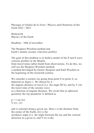
2. wave velocity. We denote by R = 6371 km the radius of the
Earth.
∆
d∆
R
p
p + dp
i
A
A’B
S
C
rb
Figure 1 – Two rays coming from the same source S with
infinitesimally different ray parameters p and p + dp. Their
angular distances of travel are ∆ and ∆+ d∆, and their travel-
times are T and T + dT . The line going through points A
and B is perpendicular to both rays.
1 Constant velocity model
Let us first assume that the wave velocity V does not vary with
depth.
1. Draw on a figure the ray going from a source S to a point A
of the surface, without any reflexion.

3. This ray could represent either the P or S phase.
2. Find the expression of the travel time T along this ray as a
function of ∆.
3. Find the expression of the incidence angle i of the ray at
point A as a function of the epicentral
distance ∆, and then show that the ray parameter is given by
p = R
V
cos
∆
2
. (2)
1/3
Physique et Chimie de la Terre / Physics and Chemistry of the
Earth 2022 / 2023
2 Linking p to T and ∆
We now turn to a more realistic model and allow for radial
variations of the waves velocities.
4. By considering two rays coming from the same source with
infinitesimally different ray parameters
p and p + dp, and travel times T and T + dT (Figure 1a),
demonstrate that
p = dT

4. d∆
. (3)
Hints : (1) Since the two rays are very close, the arcs
connecting A to A’, A to B, and B to A’
can be approximated as straight lines. (2) Show first that the
segment AB is part of a wavefront.
What does it imply for the times of arrivals at points A and B ?
5. Check that the expressions of p and T found for the constant
velocity model are consistent with
eq. (3).
3 Travel time curves and estimate of the p(∆) curves
You will find on Chamillo a file containing travel time tables
obtained from the global Earth’s seis-
mological model ak135 (either a text file, AK135tables.txt, or
an Excel spreadsheet, AK135tables.xlsx).
The files contain three columns :
— the first gives the angular distance of travel ∆ (in °) ;
— the second column gives the travel time (in seconds) of the P
phase (i.e. a P -wave travelling in
the mantle without any reflexion) ;
— the third column gives the travel time (in seconds) of the S
phase (i.e. a S-wave travelling in the
mantle without any reflexion).
6. Travel time curves :
(a) Using the programming language of your choice (Python,
Matlab/Octave, Excel, ...), make

5. a plot showing the travel times of the P and S waves as a
function of ∆.
(b) Compare with the prediction of the constant velocity model.
Can you find a P -wave velocity that allows for a good
agreement between the constant
velocity model and the observed travel times ? Comment.
7. p(∆) curves :
(a) From the travel time tables, compute the ray parameter p for
each value of ∆, for the P
and S phases.
(b) Make a plot of p as a function of ∆, for the P and S phases.
(c) Compare with the prediction of the constant velocity model.
Comment.
4 Estimating the Mantle’s VP and VS profiles using the
Herglotz-
Wiechert method
The Herglotz-Wiechert method is an ’inversion’ method
allowing to determine a vertical seismic
velocity profile from a p(∆) curve obtained from observations.
The method only works in regions where
the velocity increases with depth, and its use is therefore
restricted to regions without low-velocity
zones.
We denote by rb the radius of the bottoming point of the ray
(figure 1a), and by V (rb) the wave
velocity at r = rb.
8. From the definition of the ray parameter p (eq. (1)), find a

6. relation between p, rb, and V (rb).
2/3
Physique et Chimie de la Terre / Physics and Chemistry of the
Earth 2022 / 2023
The Herglotz-Wiechert method is based on the following
formula, which links the radius rb of the
bottoming point of a ray of angular distance ∆ to an integral
involving the ray parameter p :
rb(∆) = R exp(− 1
π
∫
∆
0
arcosh(p(∆
′)
p(∆) )d∆′) . (4)
(Note that arcosh(x) = ln (x +
√
x2 − 1).)
9. Explain qualitatively how one can use this formula together
with the results from the previous
questions to estimate the radial profiles VP (r) and VS(r).
10. Given the p v.s. ∆ tables you have obtained on question 7,

7. write a program allowing you to
(a) compute rb as a function of ∆ , using equation (4),
(b) and then compute the seismic velocity VP (rb) at each rb.
(Please hand back your program with your homework.)
Hint : To compute the integral, you can either use a built-in
integration function from you pro-
gramming language, or write a simple integration program
(either the rectangular or trapezoidal
rule can be used).
11. Use your program to compute VP and VS as functions of r,
and make a plot of the resulting
velocity profiles.
12. Compare your results with P and S velocity models you can
find on the internet (for example
from the PREM model).
3/3
Form Responses 1TimestampUntitled Question
Risk TableRisk IDID DateCause(s) Risk NameConsequenceRisk
DetailsRisk Owner (Responsible Person or
Group)ProbabilityImpactRisk ScoreResponse Action
TypeResponse Actions1Select OneSelect OneSelect OneSelect
One Select OneSelect OneSelect OneSelect One Select
OneSelect OneSelect OneSelect One Select OneSelect
OneSelect OneSelect One Select OneSelect OneSelect
OneSelect One Select OneSelect OneSelect OneSelect One
Select OneSelect OneSelect OneSelect One Select OneSelect
OneSelect OneSelect One Select OneSelect OneSelect
OneSelect One Select OneSelect OneSelect OneSelect One
Select OneSelect OneSelect OneSelect One Select OneSelect

8. OneSelect OneSelect One Select OneSelect OneSelect
OneSelect One Select OneSelect OneSelect OneSelect One
Select OneSelect OneSelect OneSelect One Select OneSelect
OneSelect OneSelect One Select OneSelect OneSelect
OneSelect One Select OneSelect OneSelect OneSelect One
Select OneSelect OneSelect OneSelect One Select OneSelect
OneSelect OneSelect One Select OneSelect OneSelect
OneSelect One Select OneSelect OneSelect OneSelect One
Select OneSelect OneSelect OneSelect One Select OneSelect
OneSelect OneSelect One Select OneSelect OneSelect
OneSelect One Select OneSelect OneSelect OneSelect One
ValuesLIKELIHOODIMPACTRISKRESPONSESelect OneSelect
OneSelect OneSelect One UnlikelyMinorAcceptable Risk:
LowAvoidLikelyModerateAcceptable Risk: MediumTransfer
Very LikelyMajorUnacceptable Risk: HighMitigate
Unacceptable Risk: Extremely HighAccept
In Week 5, your task is to create a risk management matrix that
identifies potential risks of a BallotsOnline system in the cloud,
the probability of the risk occurring, the impact if the threat
occurs, and the type of response to the risk. You will use the
Risk Management Matrix Template to complete this
task.
DO NOT write an MS word document or create your
own table. Use the template. Note: When you open the
template, use the “Risk Table” tab to populate your risks. Here
are some guidelines for the template headers.
·
Causes – What could cause a risk to occur. Example:
Weak Access Controls. Keep it general and be more
specific in the risk name. You can have multiple risk names
under a single Cause.
·
Risk Name – Give your identified risk a short but

9. somewhat specific name. Example:
Weak Passwords.
·
Consequences – Describe what will occur if the risk
becomes a reality. Example: Unauthorized users will gain
access to Ballots Online and have the ability to cast ballots.
·
Risk Details – This is where you provide specific
details about the risk and why it is important to recognize and
respond. Feel free to provide a lot of details, but remember you
are speaking to non-IT executives.
·
Risk Owner – This is the entity that generally has the
responsibility to address the risk. Owners determine the
probability and impact of a risk and what type of response is
necessary. For this exercise, enter an department (IT, Finance,
HR, etc). Most (perhaps all) for this exercise, will be addressed
by the IT department.
·
Probability – This is the likelihood of the risk
occurring. There are lots of risks to systems, but not all are in
one of the “Likely” categories. Protections already in place will
often lower the probability of a risk occurring. For example,
the probability of an internal company PC being infected with a
virus is lowered by continually updated anti-virus software.
·
Impact – This the general level of harm that would
occur IF a risk becomes reality. Minor risks may not be
addressed in the design. In other words, the impact is so low
that the response is not cost effective to implement. We just
live with it. That happens every day in the business world.
Impact is probably the biggest driver of design.

10. ·
Risk Score - This is where you determine if the risk is
acceptable or not. Risk score is a measure of
probability and
impact. If you have a risk that is Very Likely with a
Major Impact, then the Risk Score would be an Unacceptable
Risk at High or Extremely High. This means there must be a
strong response in either technology, policy, monitoring, and
infrastructure (or more likely a combination of all).
·
Response Action Type – You will either avoid (render
the risk irrelevant), mitigate (lower the probability and impact),
transfer (place the impact of the risk on another entity ;
insurance for example), or Accept (live with) all risks.
·
Response Actions – Describe the specific actions you
will take, based on the response type. If you transfer the risk,
explain how the transfer protects Ballots Online. If you Accept
the risk, explain why the impact is not worth other actions.
You will be including this information in your final report in
the form of a table, so review the competencies and make sure
your capturing the correct material. Be specific on the risks.
Hacking for example is too generic. Be specific on how
hacking can occur. Phishing, Firewall vulnerability, poor
password policies, Etc. Remember the CIAs of data
(Confidentiality, Integrity, Accuracy). Address risks that will
ensure the CIAs are protected.