Molecular water detected on the sunlit Moon by SOFIA
Poster GSA 2014
1. A Global Hot Spot Analysis (Getis-Ord Gi*) of Groundwater Storage Change
using GRACE Satellite and GIS-Based Spatial Statistical Analysis
Khalil A. Lezzaik and Adam M. Milewski
Department of Geology, University of Georgia, Athens, GA, USA
Abstract:
Global groundwater is declining as a function of over extraction, pollution, and climate change effects on
precipitation. While the dwindling of groundwater resources has been noticed, a holistic and accurate assessment of
groundwater storage change (GWSC) patterns and distributions has never been conducted given the global scale of
the assessment and the paucity of in-situ monitoring systems worldwide. Therefore, in this study, alternative remote
sensing approaches are utilized to not only delineate the distribution of global GWSC but to also observe the
relationships between climatic factors and GWSC.
NASA’s gravity recovery and climate change experiment (GRACE) mission satellite was used to derive GWSC
estimates for the purposes of identifying spatial clusters of hot spot (HS) and cold spot (CS) GWSC values. A 10° x
10° grid was utilized to generate GWSC estimates by isolating GLDAS - derived surface water parameters from
GRACE-derived total water storage change signal. Resultant GWSC estimates underwent a hot spot (Getis-Ord Gi*)
analysis to map statistically significant spatial clusters of GWSC HS/CS with a 99% confidence interval. Moreover
monthly TRMM 3B43 datasets were similarly analyzed to produce HS/CS precipitation areas that were compared to
GWSC hot spot analysis results.
In Africa, CS were located in Madagascar and the Nile river basin (Z < - 4.1). Alternatively a HS area was established
in Angola and Zambia (Z > 5.6). In Asia, CS were primarily centered in Iraq and western Iran, and in Northern India
and Nepal (Z < -7.5); whereas HS domains were dispersed in western Turkey, southern India, central Asia region and
southeast China (Z > 6). In Europe, CS regions were located in the British Isles, western French coast, eastern
Ukraine, and southwestern Russia (Z < - 3.28). Contrastingly, HS areas were located primarily in southeast Europe,
and in Portugal and southern Spain (Z > 4). In Australia, the CS area is in northwestern Australia (Z < - 8.3); whereas
a HS area was established on the central eastern coast (Z > 7).
Precipitation and GWSC HS analysis results displayed direct correspondence in several cases (e.g. Nile river basin
and eastern Ukraine), while a few areas displayed a disassociation (e.g. Portugal and southern Spain, northwestern
Australia), thus indicating an influence of anthropogenic factors on GWSC.
Objectives:
The primary objective of this study is to use GRACE ensemble datasets (arithmetic mean of JPL, CSR, and GFZ
datasets), precipitation datasets (TRMM 3b43 V7), and land surface parameters (GLDAS-2.0 NOAH) to:
1. Generate and delineate the distribution of groundwater storage change using hot spot analysis
2. Determine the relationship between precipitation estimates and groundwater storage change using spatial
regression analysis
3. Quantify groundwater storage change (GWSC) of major aquifers globally.
Methodology
CalculationofGRACE-basedGWSCusing
awaterbalanceapproach:
ΔGWSC=ΔTWSC–ΔLandParameters
Application of hot Spot analysis using
Getis-Ord Gi* Spatial Statistics, on a 1)
10°x 10° Grid and 2) Aquifer level
Assessment of the relationship between
GWSC and precipitation using OLS.
Performance of a zonal statistical
analysis to determine aquifers’TWSC
and GWSC between 2003 and 2010
Results:
1a. Global Hot Spot Analysis of GRACE- Based GWSC at 10° x 10° Grid Level
Fig. 2. Global GWSC map displaying the spatial results of the hot spot analysis on a grid level. The bright red color represent
“cold spot” areas with a spatial concentration of low GWSC values. Alternatively dark blue colors represent “hot spot” areas
with a spatial clustering of high GWSC values.
1b. Global Hot Spot Analysis of GRACE- Based GWSC at Aquifer Level
Fig. 3. Global GWSC map displaying the spatial results of the hot spot analysis on an aquifer level. The red numbering refers
to the following aquifer systems: 1) Central California Valley 2) Cambrio-Ordovician 3) Ogallala High Plains 4) Gulf Coastal
5) Atlantic Coastal 6) Amazonas 7) Maranhao 8) Guarani-Mercosul 9) Karoo 10) Lower Kalahari 11) Upper Calahari 12)
Congo 13) Lac Chad 14) Iullemeden – Irhazer 15) Iullemeden-Irhazer 16) Northwestern Sahara 17) Murzuk-Djado 18) Nubian
19) Arabian 20) Ogaden-Juba 21)Umm Ruwaba 22) Indus 23) Indus-Ganges-Brahmaputra 24) Northern Caucasus 25) Tarim
26) Song-Liao Plain 27) Northern China 28) Canning Basin 29) Artesian Grand Basin.
Tab. 2. A display of calculated cumulative GWSC between
January 2003 and December 2010 of major groundwater
aquifers worldwide. Total global GWSC was estimated to be in
excess of 9986 𝑘𝑚3
. With the exception of notable aquifers
known for their high depletion rates – Indus Ganges Basin,
Ogallala High Plains Aquifer, Northwestern Sahara Aquifer
System – the majority of large scale groundwater systems
appear to be gaining water storage.
Fig. 1. Diagram displaying the different methodological procedures in sequential order.
2. Statistical Correlation Between Precipitation and GWSC
Aquifer / Basin Adjusted 𝑹 𝟐
Amazonas Basin 0.99
Arab Aquifer System 0.92
Artesian Grand Basin 0.93
Atlantic Ocean and Coastal Plains Aquifer 0.96
Cambrio-Ordovician Aquifer System 0.96
Canning Basin 0.98
Central California Valley Aquifer System 0.61
Congo Basin 0.94
Guarani (or Mercosul) Aquifer System 0.99
High Kalahari Cuvelai Basin 0.98
Indus Basin 0.98
Indus-Gange-Brahmaputra Basin 0.22
Iullemeden – Irhazer Aquifer System 0.97
Karoo Basin 0.97
Lac Chad Basin 0.88
Low Kalahari – Stampriet Basin 0.27
Maranhão Basin 0.95
Murzuk – Djado Basin 0.58
Northern Caucasus Basin 0.96
Northern China Aquifer System 0.98
North-Western Sahara Aquifer System 0.84
Nubian Aquifer System 0.99
Ogaden-Juba Basin 0.98
Ogallala Aquifer (High Plains) 0.99
Song-Liao Plain 0.98
Taoudeni – Tanezrouft Basin 0.98
Tarim Basin 0.69
Umm Ruwaba Aquifer 0.5
Fig. 4. Global map displaying the relationship between precipitation (explanatory variable) and GWSC
(dependent variable) based on residual standard derivation estimates generated by an ordinary least squares
regression model. Light yellow, blue, and green colors correspond to areas with high precipitation-GWSC
correlation. Dark red and blue colors correspond to areas with low precipitation-GWSC correlation.
Tab. 1. Adjusted R-squared values reflecting
the correlation between precipitation and
GWSC in different aquifer systems globally.
3. Quantification of Cumulative GWSC in Major Large Aquifer Globally between 2003 and 2010
Aquifer/ Basin Area (sq. km) GWSC (water column, cm) GWSC (volumetric, km3)
Northern Caucasus Basin 288825 -66.53 -192.17
Central California Valley Aquifer System 419040 -35.10 -147.10
Umm -Ruwaba Aquifer 470534 18.72 88.10
Song - Liao Plain 477958 8.80 42.08
Low Kalahari - Stampriet Basin 494316 6.40 31.64
Iullemeden -Irhazer Aquifer System 553636 25.19 139.47
Cambro-Ordovician Aquifer System 614542 40.91 251.39
Murzuq Djado Basin 617341 -6.02 -37.13
Karoo Basin 674316 11.54 77.78
Tarim Basin 711981 14.38 102.35
Indus Basin 752482 -20.03 -150.73
Ogallala High Plains Aquifer 766478 -32.77 -251.18
Maranhao Basin 777693 -77.69 -604.22
High Kalahari Cuvelai 987577 86.15 850.83
North Western Sahara Aquifer System 1096982 -4.41 -48.41
Indus - Ganges - Brahamaputra Basin 1142907 -3.77 -43.06
Lac Chad Basin 1153914 13.34 153.91
Canning Basin 1249850 -2.67 -33.33
Ogaden - Juba Basin 1468133 24.96 366.39
Congo Basin 1589759 122.91 1954.00
Taoudeni -Tanezrouft Basin 1851101 33.22 614.85
Nubian Aquifer System 1979482 25.13 497.54
Arab Aquifer Basin 1987873 -5.31 -105.62
Atlantic Ocean and Gulf Coastal Plains Aquifer 2112984 108.67 2296.08
Guarani - Mercosul Aquifer System 2240517 110.65 2479.22
Amazona Basin 3534833 -91.71 -3241.65
Artesian Grand Basin 5918896 82.71 4895.25
Total Groundwater Storage Change 35933950 388 9986
Future Work
• Examining the relationship between GWSC and
environmental variables such as vegetative cover,
soil, and topography using spatial exploratory
regression.
Acknowledgments
• The Geological Society of America
• University of Georgia Office of the Vice President
for Research
• Watts-Wheeler Scholarship Fund