VIP Call Girls Service Hitech City Hyderabad Call +91-8250192130
lecture 2 parametric yield.pdf
1. 1
Lecture 2: Parametric Yield
Spanos
EE290H F05
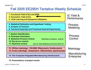
Fall 2005 EE290H Tentative Weekly Schedule
1. Functional Yield of ICs and DFM.
2. Parametric Yield of ICs.
3. Yield Learning and Equipment Utilization.
4. Statistical Estimation and Hypothesis Testing.
5. Analysis of Variance.
6. Two-level factorials and Fractional factorial Experiments.
7. System Identification.
8. Parameter Estimation.
9. Statistical Process Control. Distribution of projects. (week 9)
10. Run-to-run control.
11. Real-time control. Quiz on Yield, Modeling and Control (week 12)
12. Off-line metrology - CD-SEM, Ellipsometry, Scatterometry
13. In-situ metrology - temperature, reflectometry, spectroscopy
14. The Computer-Integrated Manufacturing Infrastructure
15. Presentations of project results.
Process
Modeling
Process
Control
IC Yield &
Performance
Metrology
Manufacturing
Enterprise
2. 2
Lecture 2: Parametric Yield
Spanos
EE290H F05
IC Yield and Performance (cont.)
• Defect Limited Yield
• Definition and Importance
• Metrology
• Modeling and Simulation
• Design Rules and Redundancy
• Parametric Yield
• Parametric Variance and Profit
• Metrology and Test Patterns
• Modeling and Simulation
• Worst Case Files and DFM
• Equipment Utilization
• Definition and NTRS Goals
• Measurement and Modeling
• Industrial Data
• General Yield Issues
• Yield Learning
• Short loop methods and the promise of in-situ metrology
3. 3
Lecture 2: Parametric Yield
Spanos
EE290H F05
IC Structures can be highly Variable
Transistor
Interconnect
Variability will impact performance
4. 4
Lecture 2: Parametric Yield
Spanos
EE290H F05
What is Parametric Yield?
• When devices (transistors) do not have the
exact size they were designed for,
• when interconnect (wiring) does not have the
exact values (Ohms/μm, Farads/μm2, etc.) that
the designer expected,
• when various structures (diffused layers, contact
holes and vias, etc.) are not exactly right,
• the circuit may work, but
• performance (speed, power consumption, gain,
common mode rejection, etc.) will be subject to
statistical behavior...
5. 5
Lecture 2: Parametric Yield
Spanos
EE290H F05
What are the Parametric Yield Issues?
• Binning and Impact on Profitability
• The Process and Performance Domains
– Characterizing the Process Domain
– Identifying Critical Variables
– Modeling Process Variability
– Associated (Statistical) Metrology
• Process Variability and the Circuit Designer
• Design for Manufacturability Methods
• A Global (re)view of Yield
6. 6
Lecture 2: Parametric Yield
Spanos
EE290H F05
What is the Critical Dimension?
CD
Gate is typically made out of Polysilicon
7. 7
Lecture 2: Parametric Yield
Spanos
EE290H F05
Basic CD Economics
(D. Gerold et al, Sematech AEC/APC, Sept 97, Lake Tahoe, NV)
8. 8
Lecture 2: Parametric Yield
Spanos
EE290H F05
Application of Run-to-Run Control at Motorola
Dosen = Dosen-1 - β (CDn-1 - CDtarget)
(D. Gerold et al, Sematech AEC/APC, Sept 97, Lake Tahoe, NV)
9. 9
Lecture 2: Parametric Yield
Spanos
EE290H F05
CD Improvement at Motorola
σLeff reduced by 60%
(D. Gerold et al, Sematech AEC/APC, Sept 97, Lake Tahoe, NV)
10. 10
Lecture 2: Parametric Yield
Spanos
EE290H F05
Why was this Improvement Important?
600k APC investment, recovered in two days...
11. 11
Lecture 2: Parametric Yield
Spanos
EE290H F05
Process and Performance Domains
• CD is not the only process variable of interest…
• Speed is not the only performance of interest…
• In general we have a mapping between two multi-
dimensional spaces:
CD
Resistivities
Conductance of contacts and Vias
Dielectric capacitance per unit area...
Speed
Power
...
12. 12
Lecture 2: Parametric Yield
Spanos
EE290H F05
So, what to do?
Process
Electrical
Circuit
Performance
What performance is important?
What Process/Layout parameters can we
change to satisfy critical performance specs?
How to simulate performance variation?
How to design a circuit that is immune to
variation?
What electrical parameters matter?
How can we set reasonable specs on those?
What process parameters to measure?
How to reduce Process Variability?
13. 13
Lecture 2: Parametric Yield
Spanos
EE290H F05
Translating Specifications between Domains
• Performance Specs, imposed by the market, translate to
an “acceptability region” in the process domain.
• This “acceptability region” is also known as the Yield
Body (YB).
• The Yield Body can be mapped into either domain.
14. 14
Lecture 2: Parametric Yield
Spanos
EE290H F05
So what is Parametric Yield?
• One is interested in mapping and in maximizing the
overlap between YB and PS.
• This can be accomplished in various ways.
• first, we should be able to measure (characterize) the Process
Spread (PS).
• then, one has to figure the mapping from Process to Performance!
• Finally, one needs design tools to manipulate the above.
15. 15
Lecture 2: Parametric Yield
Spanos
EE290H F05
Parametric Test Patterns
Typically on scribe lanes or
in “drop-in” test ICs.
E-test measurements:
- transistor parameters
- CDs
- Rs
- Rc
- small digital and analog
blocks
- ring oscillators
Special
Test
IC
IC
IC
IC IC
IC
IC
IC
IC
17. 17
Lecture 2: Parametric Yield
Spanos
EE290H F05
There is no agreement about Interconnect
Parameters...
An Extraction Method to Determine Interconnect Parasitic Parameters, C-J Chao, S-C Wong, M-J Chen, B-K Liew, IEEE
TSM, Vol 11, No 4. Nov 1998.
21. 21
Lecture 2: Parametric Yield
Spanos
EE290H F05
Statistical Metrology for CDs
Spatial
Random/Deterministic
Within Die
Among Die
Among Wafers
Causal
Equipment Recipe
?
Other
Response from Equipment A
Random/Deterministic
Where does variability come from?
What are its spatial components?
22. 22
Lecture 2: Parametric Yield
Spanos
EE290H F05
Data Collection
• Electrical Measurements
facilitate data collection.
• Raw data contains
confounded variability
components from the
entire “short loop”
process sequence.
wafer
CD
You can “see” the boundaries
of the stepper fields!
23. 23
Lecture 2: Parametric Yield
Spanos
EE290H F05
Nested Variance – A Simple Model
CDijkl = μ + fi + wj + lk + Ll + σ
True mean
Across-field
Across-wafer
Across-lot
Lot-to-lot
Random
CD variation can be thought of as nested systematic
variations about a true mean: Spatial components
Field
Wafer
Lot
Jason Cain, SPIE 2003
24. 24
Lecture 2: Parametric Yield
Spanos
EE290H F05
Experimental Design
• Use a mask with densely grouped test features
to explore spatial variability.
• Electrical linewidth metrology (ELM) chosen as
primary metrology due to its high speed.
• A fabrication process based on a standard 248
nm lithography process was used to print test
wafers.
25. 25
Lecture 2: Parametric Yield
Spanos
EE290H F05
Test Mask Design
• Mask design consists of a 22x14 array of test
modules
• Module has CD structures (ELM, CD-SEM,
OCD) in varying pitch, orientation, and OPC use.
• Density of structures allows detailed variance
maps using an “exhaustive” sampling plan.
• Three feature types measured for each module
for every field on the wafer (all no-OPC).
26. 26
Lecture 2: Parametric Yield
Spanos
EE290H F05
Test Mask Design (cont)
SEM
Lines
ID: XXN
Grating
Horz Iso
W/S= 180/
1000
Grating
Vert Iso
W/S= 180/
1000
Grating
Horz Iso
W/S= 180/
360
Grating
Vert Iso
W/S= 180/
360
Grating
Horz
Medium
W/S = 180/
240
Grating
Vert Medium
W/S = 180/
240
Grating
Horz Dense
W/S = 180/
180
Grating
Vert Dense
W/S = 180/
180
DUT1
Vert
DUT2
Vert
DUT3
Horz
DUT4
Horz VDP
DUT5
Horz
DUT6
Horz
DUT7
Vert
DUT8
Vert
1 2 3 4 5 6 7 8 9 10 11 12 13 14 15
31
30 29 28 27 26 25 24 23 22 21 20 19 18 17 16
32
SEM
Lines
ID: XXO
DUT1
Vert
DUT2
Vert
DUT3
Horz
DUT4
Horz VDP
DUT5
Horz
DUT6
Horz
DUT7
Vert
DUT8
Vert
1 2 3 4 5 6 7 8 9 10 11 12 13 14 15
31
30 29 28 27 26 25 24 23 22 21 20 19 18 17 16
32
SEM
Lines
CF_LENS coma/flare
CD_LIN linearity
MEFH
MEF
Probe pads
ELM CD Patterns
OCD Patterns
27. 27
Lecture 2: Parametric Yield
Spanos
EE290H F05
Across-Field Systematic Variation –
Mask Errors
Average Field
Scaled Mask Errors
Non-mask related across-
field systematic variation
Calculate average field to see across-field systematic variation
Use mask measurements to decouple scaled mask errors from
non-mask related systematic variation
- =
σ2 = (2.57 nm)2 σ2 = (1.78 nm)2 σ2 = (1.85 nm)2
Scan
Slit
28. 28
Lecture 2: Parametric Yield
Spanos
EE290H F05
Optimizing Mask Error Scaling Factor for ELM
Mask error scaling factor optimized to minimize residuals
when mask errors are removed from average field.
Mask Errors
→ Aerial Image
→ Resist Pattern
→ Trim Etch
→ Poly Etch
→ Electrical
Measurement
Electrical MEF
Mask Error Scaling Factor
Optical MEF expected to
be ~1.2
0.7
29. 29
Lecture 2: Parametric Yield
Spanos
EE290H F05
Across-Field Systematic Variation
Average field
with mask errors
removed
Polynomial model of
across-field
systematic variation
Residuals
=
-
Polynomial model used to capture across-field systematic
variation (inferred from examination of data):
CD(Xf,Yf) = aXf
2 + bYf
2 + cXf + dYf
σ2 = (1.85 nm)2 σ2 = (1.23 nm)2 σ2 = (1.38 nm)2
Scan
Slit
31. 31
Lecture 2: Parametric Yield
Spanos
EE290H F05
Across-Wafer Systematic Variation
• There is a distinct local drop in CD value in the wafer center,
most likely linked to the way the develop fluid is dispensed.
• A bi-variate Gaussian function was fitted to the data to
remove this effect.
- =
Across-Wafer
Systematic Variation
Bivariate Gaussian
Model
Remaining Across-Wafer
Systematic Variation
σ2 = (2.46 nm)2 σ2 = (0.52 nm)2 σ2 = (2.39 nm)2
32. 32
Lecture 2: Parametric Yield
Spanos
EE290H F05
Across-Wafer Systematic Variation
The remaining across-wafer systematic variation was removed
using a polynomial model:
CD(Xw,Yw) = aXw
2 + bYw
2 + cXw + dYw + eXwYw
- =
Across-Wafer Systematic
Variation with bivariate
Gaussian removed
Polynomial Model Remaining Across-Wafer
Systematic Variation
σ2 = (2.39 nm)2 σ2 = (1.39 nm)2 σ2 = (1.95 nm)2
33. 33
Lecture 2: Parametric Yield
Spanos
EE290H F05
Systematic Variation Model Summary
• Across-field systematic variation:
– Mask errors (magnified scaling factor) removed
– Polynomial terms in X and Y across the field
• Across-wafer systematic variation:
– Across-field systematic variation removed
– Bivariate Gaussian for spot effect (likely linked to develop effect)
– Polynomial terms in X and Y across the wafer
34. 34
Lecture 2: Parametric Yield
Spanos
EE290H F05
Reduced Sampling Plan Candidates
Plan 1: 920 measurements Plan 2: 900 measurements
Plan 3: 927 measurements Plan 4: 785 measurements
Each plan requires roughly one hour of measurement time
(Exhaustive plan had 21,252 measurements, requiring 25 hours)
35. 35
Lecture 2: Parametric Yield
Spanos
EE290H F05
Comparison of Reduced Sampling Plans
Plan 1 offers the best estimate of across-wafer variation
without compromising the quality of the across-field estimate.
Across-Field
Across-Wafer
Unable
to
estimate
Unable
to
estimate
Unable
to
estimate
Unable
to
estimate
Unable
to
estimate
Unable
to
estimate
36. 36
Lecture 2: Parametric Yield
Spanos
EE290H F05
Statistical Metrology for Dielectrics
Rapid Characterization and Modeling of Pattern-Dependent Variation in Chemical-Mechanical Polishing
Brian E. Stine, Dennis O. Ouma, Member, IEEE, Rajesh R. Divecha, Member, IEEE, Duane S. Boning, Member, IEEE,
James E. Chung, Member, IEEE, Dale L. Hetherington, Member, IEEE, C. Randy Harwood,
O. Samuel Nakagawa, and Soo-Young Oh, Member, IEEE, IEEE TSM, VOL. 11, NO. 1, FEBRUARY 1998
37. 37
Lecture 2: Parametric Yield
Spanos
EE290H F05
Dielectric Thickness vs Position in Field
Studies like this can be used
to complement “random”
variability with the
deterministic, pattern
dependent variability.
The combination of the two
leads to simulation tools that
can predict very well the
“spread” of circuit
performances.
38. 38
Lecture 2: Parametric Yield
Spanos
EE290H F05
Impact of Process Variability to Circuit
Performance
• Obviously, not everything in the process impacts
the Circuit Performance.
• Studies have tried to focus on the most
important process parameters.
• CD is clearly one of them.
39. 39
Lecture 2: Parametric Yield
Spanos
EE290H F05
Impact of Pattern-Dependent Poly-CD Variation
Simulating the Impact of Pattern-Dependent Poly-CD Variation on Circuit Performance, Stine, et al, IEEE TSM, Vol 11, No
4, November 1998
Use basic Optical Model to determine “actual” pattern...
43. 43
Lecture 2: Parametric Yield
Spanos
EE290H F05
Modeling Spatial Matching
• Component Matching is an aspect of process
variability that affects the yield of Analog
Circuits:
– D-A converters: capacitor matching.
– Diff amplifiers, current sources: transistor matching.
44. 44
Lecture 2: Parametric Yield
Spanos
EE290H F05
Circuit Element “Matching” Models
• In order to describe matching one needs a “spatial”
distribution.
• In this case location, as well as distance are factors that
will affect process (and performance) variability.
• Several models have been created, either empirically, or
by taking into account detailed device parameters.
45. 45
Lecture 2: Parametric Yield
Spanos
EE290H F05
Pelgrom’s Model
1 2
1A 2A
2B 1B
L
W
L
W
L
W
Dx
Dx
Dy
σ2(ΔP) = A2
p/WL + S2
pD2
x
σ2(ΔP) = A2
p/2WL + S2
pD2
xD2
y/wafer diameter
Variance inversely proportional to area, proportional to distance2.
47. 47
Lecture 2: Parametric Yield
Spanos
EE290H F05
Example on Variance in Element Array
1
2
3
4
5
6
7
8
9
10
48. 48
Lecture 2: Parametric Yield
Spanos
EE290H F05
Example of Variance vs. size, distance
σ2
ΔR/R vs 1/L
σ2
ΔR/R vs D2
49. 49
Lecture 2: Parametric Yield
Spanos
EE290H F05
Simulating Parametric Yield
• The process domain can be mapped to the performance domain
through random exploration.
• The Yield can then be estimated as Y= Np/N.
• Though this estimate converges rather slowly, it does have some
nice properties.
50. 50
Lecture 2: Parametric Yield
Spanos
EE290H F05
Monte Carlo - the speed of Convergence
• Since Y is an estimate of a random variable, bounds for the
actual value of Y are given by the general Tchebycheff
inequality:
P{|Yest-Y| > kσ} < 1/k2
• Since each random experiment can be seen as a Bernoulli
trial with Y probability of success, then if N is large and Y(1-
Y)N>6 (or so), we can employ the approximation:
μY = Y
σ2
Y=Y(1-Y)/N
• The estimation accuracy is independent of the
dimensionality of the process domain.
definitions: Y: actual yield, N: number of Monte Carlo trials, μY, σ2
Y are the mean
and variance of the estimated yield Yest.
53. 53
Lecture 2: Parametric Yield
Spanos
EE290H F05
Yield Simulation Example
N = 100, Np = 59
Y = 0.59, σ2
y=Y(1-Y)/N = 0.052
Y = 0.59 +/-0.15 => 0.44 < Y < 0.74
54. 54
Lecture 2: Parametric Yield
Spanos
EE290H F05
Next Time on Parametric Yield
• Current and Advanced DFM techniques
– The role of process simulation (TCAD)
– Complete Process Characterization
– Worst Case Files
– Statistical Design
• The economics of DFM