UTA AE5305 Fall 2023 Homework 1

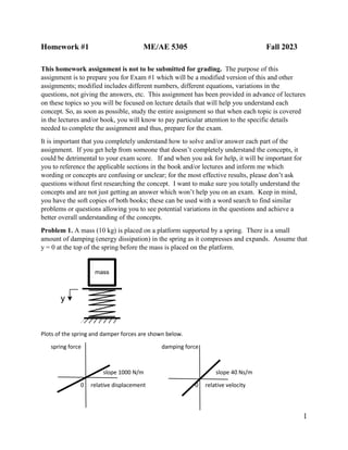
1. 1
Homework #1 ME/AE 5305 Fall 2023
This homework assignment is not to be submitted for grading. The purpose of this
assignment is to prepare you for Exam #1 which will be a modified version of this and other
assignments; modified includes different numbers, different equations, variations in the
questions, not giving the answers, etc. This assignment has been provided in advance of lectures
on these topics so you will be focused on lecture details that will help you understand each
concept. So, as soon as possible, study the entire assignment so that when each topic is covered
in the lectures and/or book, you will know to pay particular attention to the specific details
needed to complete the assignment and thus, prepare for the exam.
It is important that you completely understand how to solve and/or answer each part of the
assignment. If you get help from someone that doesn’t completely understand the concepts, it
could be detrimental to your exam score. If and when you ask for help, it will be important for
you to reference the applicable sections in the book and/or lectures and inform me which
wording or concepts are confusing or unclear; for the most effective results, please don’t ask
questions without first researching the concept. I want to make sure you totally understand the
concepts and are not just getting an answer which won’t help you on an exam. Keep in mind,
you have the soft copies of both books; these can be used with a word search to find similar
problems or questions allowing you to see potential variations in the questions and achieve a
better overall understanding of the concepts.
Problem 1. A mass (10 kg) is placed on a platform supported by a spring. There is a small
amount of damping (energy dissipation) in the spring as it compresses and expands. Assume that
y = 0 at the top of the spring before the mass is placed on the platform.
mass
time
y
y
0
Plots of the spring and damper forces are shown below.
spring force damping force
slope 1000 N/m slope 40 Ns/m
0 relative displacement 0 relative velocity

2. 2
Draw the free body diagram for the components in this system assuming a damper is parallel to
the spring; include the d’Alembert force on the mass. Verify that you get the following
component equations using g for gravity.
(1) 𝟏𝟎𝒚̈ + 𝑭𝒅 + 𝑭𝒔 − 𝟏𝟎𝒈 = 𝟎
(2) 𝑭𝒅 = 𝟒𝟎𝒚̇ 𝒅𝒂𝒎𝒑𝒊𝒏𝒈 𝒇𝒐𝒓𝒄𝒆, Ns/m
(3) 𝑭𝒔 = 𝟏𝟎𝟎𝟎𝒚 𝒔𝒑𝒓𝒊𝒏𝒈 𝒇𝒐𝒓𝒄𝒆, 𝑵/𝒎
(a) There are 3 equations; so, there must also be 3 unknowns. Verify that the 3 unknowns are y,
Fd and Fs. Make sure you understand why 𝑦̇ and 𝑦̈ are not counted as unknowns also.
(b) Explain how you know that each of these equations is linear.
(c) Explain how you know that the order of this system of equations is 2nd
order.
(d) Assume the mass is gently placed on the platform and the platform settles down compressing
the spring. Verify mathematically that the final value of the force pushing down on the spring
will be 10g N; use commonsense to explain why this final value is correct.
(e) Verify mathematically that the final value of y will be 0.01g m.
(f) You are to solve for the transfer function for the spring force Fs corresponding to the input g .
Convert the differential equations to algebraic equations using the Laplace operator and solve
for Fs verifying that the transfer function is
10000
10𝑠2 + 40𝑠 + 1000
(g) Verify that the eigenvalues of this system are −2 ± 𝑗9.798; that the damped natural
frequency is 9.798 rad/s; that the undamped natural frequency is 10 rad/s; that the damping ratio
is 0.2.
(h) Considering the initial and final values of y and the duration of the response and assuming
g = 9.81 m/s2
, explain why the estimates of y(t) on the graph below are potentially valid but the
plot with oscillations is the most likely case.
0 2.5 time, s
0.0981
y(t), m

3. 3
(i) Assume the stiffness of the spring is nonlinear as shown below.
spring force
𝐹
𝑠 = 103911𝑦3
0 y
Assume the mass is at rest (equilibrium) setting on the platform. Assume someone taps on the
top of the mass with a hammer and causes the mass to start to vibrate up and down. Verify that a
linear approximation for the spring force should be
𝐹
𝑠 ≈ 3000𝑦 − 196.2
(j) Using the linear approximation in (i) for the spring force, verify that the approximate
damping ratio of the nonlinear system is 0.12 and the damped natural frequency is 17.2 rad/s.
Intuitively, why do you think the oscillation frequency with the nonlinear spring is so much
greater than the frequency with the linear spring?
(k) Since the system of equations is 2nd
order, two state variables are required for a numerical
simulation of the dynamics of this system; make sure you understand why this is true. We know
that there are an infinite number of ways these two state variables can be defined. Explain why
the following definitions for the state variables can be used to express either the linear or
nonlinear equations in state variable format.
x1 = y x2 = 𝑦̇
(l) Using the definitions in (k), verify the validity of the following equations for the derivatives
of x1 and x2 if the nonlinear spring equation is used in the model.
𝑥̇1 = 𝑥2
𝒙̇𝟐 = −𝟒𝒙𝟐 − 𝟏𝟎𝟑𝟗𝟏. 𝟏𝒙𝟏
𝟑
+ 𝒈

4. 4
Problem 2. The schematic of a water tank is shown below. At time t =0, the height H of water in
the tank is 2 m. At t=0 water starts flowing into the tank at a constant rate of Qi(t) = 8 m3
/s and
flowing out with a flow rate of Qo; note, Qo is a function of H. The equations for this system are
(1) 8𝐻̇ (𝑡) = 𝑄𝑖 − 𝑄𝑜(𝑡) 𝐻(0−) = 2
(2) 𝑄𝑜(𝑡) = 0.4𝐻(𝑡)
Qi = 8 m3
/s
H
H(t)
0 time
Qo
(a) There are 3 variables in these equations; what are they? Since we only have 2 equations, only
2 of the variables can be considered unknowns; explain why Qo and H have to be these two
variables that are unknown.
(b) Commonsense tells us that the height of the water in the tank will start at the initial height
and end at some constant value when the flow in and the flow out are the same. Since 𝐻̇ is zero
when 𝐻 is constant, we can solve the two equations for the final value of 𝐻. Verify that the final
value of H is 20 m.
(c) Considering the initial and final values of 𝐻 and the approximate time to get to the final value
of H, explain why the estimate of H(t) on the graph below is a potentially valid estimate.
H(t)
20
2
0 100 t, s
(d) Substitute (2) into (1) and get a 1st
order differential equation for H(t) with H(t) being the
only unknown; be sure to substitute the value for Qi. Verify the following result:
𝐻̇ + 0.05𝐻 = 1 𝐻(0−) = 2

5. 5
(e) Since the equation in (d) is only 1st
order, you can rewrite it in the format for a separation of
variables solution for H(t); verify the following result:
∫
1
1−0.05𝐻
𝑑𝐻
𝐻(𝑡)
2
= ∫ 𝑑𝑡
𝑡
0
(f) Verify that the integrals in (e) give
𝐻(𝑡) = 20 − 18𝑒−0.05𝑡
(g) Differentiate the equation in (f) to get 𝐻̇ (𝑡). Then verify that the solution in (f) is correct by
substituting 𝐻(𝑡) and 𝐻̇ (𝑡) into your original equation found in (d).
(h) Verify that the equation for H(t) in (f) gives the correct initial condition of 2 by substituting
t = 0.
(i) Verify that the equation for H(t) in (f) gives the correct final value of 20 by substituting t = ∞.
(j) Use Euler’s integration with a time increment of 5 seconds to numerically solve for H(t) at t
= 5 seconds and compare the result with the exact solution in (f) for H(t) at t = 5. Verify that
the exact solution is 5.9816 and that using the Euler method the solution is 6.50 which is an 8.7%
error.
Problem 3. Draw a graph showing each of the following two complex numbers and then verify
that the magnitude and angle of the following ratio of complex numbers are 1.166 and -1.18 rad
respectfully by finding the magnitudes and angles of each complex number separately.
−5+𝑗3
−4−𝑗3
Problem 4. We are interested in having a simple single mass lumped model for the vibration
displacement y(t) at the end of a slender cantilevered beam attached to a structure with vertical
displacement u(t).
u(t) L y(t) b= 0.1
𝜃 h=0.04
Using the stiffness matrix on page 4-14 in the book, verify that the equations simplify to
−𝑀𝑒𝑦̈ = 𝑎𝑢 + 𝑎𝑦 − 𝑏𝜃
0 = 𝑏𝑢 − 𝑏𝑦 + 𝑐𝜃
Verify that eliminating 𝜃 leads to
𝑀𝑒𝑦̈ +
3𝐸𝐼
𝐿3
𝑦 =
3𝐸𝐼
𝐿3
𝑢
b=0.1 m, h=0.04 m, A=bh m2
, L=3 m, 𝜌 = 7,800
𝑘𝑔
𝑚3
, 𝐸 = 2.07 ∗ 1011
, I=bh3
/12
Verify that the differential equation for y(t) is 𝑦̈ + 540𝑦 = 540𝑢

6. 6
Problem 5. The input to the system shown below is the force Fi(t). The two identical wheels with
radius r roll without slip. Each wheel has mass Mw and rotational inertia 𝐽 =
𝑀𝑤𝑟2
2
; the connector
bars each have mass Mb. The spring is linear with stiffness K and the viscous damper is linear with
coefficient b. The bearings at the center of the wheels are frictionless.
5.1 Verify the free body diagram shown below using d’Alembert forces and moments.
v u ∅
𝜃 k Fi
b
(𝑀𝑤 + 𝑀𝑏)𝑣̈ v u (𝑀𝑤 + 𝑀𝑏)𝑢̈ J∅̈
𝐽𝜃̈ Fs Fs Fi
Fd Fd
F1 v u F2
5.2 Sum the moments about the wheel/surface contact points and write the force equations to get
the following component equations. Note, gravity forces are not shown since there is no vertical
motion.
𝑟(𝑀𝑤 + 𝑀𝑏)𝑣̈ + 𝐽𝜃̈ − 𝑟(𝐹
𝑠 + 𝐹𝑑) = 0
𝑟(𝑀𝑤 + 𝑀𝑏)𝑢̈ + 𝐽∅̈ + 𝑟(𝐹𝑠 + 𝐹𝑑) − 𝑟𝐹𝑖 = 0
𝐹
𝑠 = 𝑘(𝑢 − 𝑣)
𝐹𝑑 = 𝑏(𝑢̇ − 𝑣̇)
𝑣 = 𝑟𝜃
𝑢 = 𝑟∅
List the unknowns in these equations.
5.3 Verify that the component equations combine and simplify to the following simultaneous
equations:
(1.5Mw + M𝑏)𝒗̈ + 𝒃𝒗̇ + 𝒌𝒗 = 𝒃𝒖̇ + 𝒌𝒖
(1.5Mw + M𝑏)𝒖̈ + 𝒃𝒖̇ + 𝒌𝒖 = 𝒃𝒗̇ + 𝒌𝒗 + 𝑭𝒊

7. 7
5.4 Explain why the four state variables shown below are required to simulate this system using
ode45; what are the derivative equations for these state variables?
𝒙𝟏 = 𝒗 𝒙𝟐 = 𝒗̇ 𝒙𝟑 = 𝒖 𝒙𝟒 = 𝒖̇
5.5 The following code has been written to simulate this system and plot the spring force
assuming the input force input 100𝑒−2𝑡
. Be able to explain the purpose of each line of the code
and confirm, by executing the code, the results of the simulation which is the plot shown below.
function Homework_1_5305_Fall_2023
Mw=20;Mb=5;K=3500;b=350;
[t,x]=ode45(@eqns,[0 3],[0 0 0 0]);
fs=3500*(x(:,3)-x(:,1));
plot(t,fs,'r','linewidth',3)
xlabel('time s','fontsize',20)
ylabel('spring force, N','fontSize',20)
grid
function dx = eqns(t,x)
dx=zeros(4,1);
v=x(1);vd=x(2);u=x(3);ud=x(4);
Fi=100*exp(-2*t);
dx(1)=vd;
dx(2)=(b*ud+K*u-K*v-b*vd)/(1.5*Mw+Mb);
dx(3)=ud;
dx(4)=(b*vd+K*v-K*u-b*ud+Fi)/(1.5*Mw+Mb);
end
end

8. 8
Problem 6. Consider the differential equation below.
𝑦̈ + 2𝑦̇ + 0.2√𝑦 = 0.8 𝑦(0−) = 9 𝑦̇(0−) = 0.5
(a) Verify that the final value of y(t) is 16.
(b) Since y starts at 9 and ends at 16, verify that a straight-line approximation for √𝑦 that would
be appropriate for linearizing this differential equation is √𝑦 ≈
1
7
𝑦 +
12
7
(c) Replace √𝑦 in the differential equation with your straight-line approximation for √𝑦 to get a
linear approximation for the original 2nd
order differential equation. Verify that the linear
approximation for the differential equation is
ÿ + 2ẏ + 0.0286y = 0.457 y(0−) = 9 ẏ(0−) = 0.5
(d) Suppose the initial value of y is 16, not 9. Explain why the assumption is reasonable that
y(t) is always in the neighborhood of 16. Since y is always close to 16, verify using the Taylor
series that an appropriate linear approximation for the differential equation is
ÿ + 2ẏ + 0.025y = 0.4 y(0−) = 16 ẏ(0−) = 0.5
Comment on the simplicity of using the Taylor series compared to the 2-point method.
(e) Compare the resulting equations in (c) and (d). What are the differences and are they
significant? For example, demonstrate that the final values in both are correct.