1. 113
April 8, 2014
TA: Ozgur
Group 2
LOE: 5 hours
IC-AFM lab
Introduction
The purpose of this lab was to gain experience using the Veeco Digital Instruments CP-II
and Innova SPM hardware and software in the intermittent and contact AFM modes. To begin
the lab, a gold nanoparticle sample was loaded into and prepared for the contact mode of the
AFM. Two scans were taken and measurements were taken to determine the diameter of the
particles and the center-to-center distance between the particles. The gold sample was then
unloaded and the cicada wing sample was loaded onto the AFM stage. The same measurements
listed above were taken again. The system was shut down and then prepared for the intermittent
contact mode. Scans of both samples were taken which produced images and the measurements
listed above for each sample. The system was shut down and the appropriate equipment was put
away.
Results
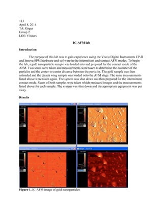
Figure 1. IC-AFM image of gold nanoparticles

2. Figure 2. IC-AFM image of gold nanoparticles (zoomed-in from Figure 1)
Figure 3. IC-AFM image of gold nanoparticles with profilometer scan

3. Figure 4. C-AFM image of cicada wing with 10µm scan range
Figure 5. C-AFM image of cicada wing with profilometer scan and 2.75 µm scan range

4. Figure 6. C-AFM image of gold nanoparticles with 0.76µm scan range
Figure 7. C-AFM image of gold nanoparticles with 3.58µm scan range

5. Table 1. AFM measurements of two samples
Conclusion
In Atomic Force Microscopy (AFM), the tip of the cantilever is lowered close to the
surface of the sample, causing an interaction of force defined by Hooke’s law between the tip
and the sample. This force causes the cantilever to be deflected which is measured by a laser
being reflected off the top of the cantilever onto a detector, which in the case of this lab is a
piezoelectric scanner. The results are translated into an image for which the resolution can be
improved using imaging software. In non-contact AFM (NC-AFM), the tip of the probe stays at
a distance of tens to hundreds of angstroms away from the surface which minimizes frictional
forces. Since NC-AFM utilizes stiff cantilevers and small forces, the resulting small signal must
be coupled with a sensitive detector for images with good resolution and accurate measurements.
NC-AFM uses attractive forces between the tip and the sample. One attractive force due to the
interaction between the probe and sample is the spring force. The spring force is mathematical
defined by Hooke’s law (F = -kx). F is the force applied, in this case to the cantilever, k is the
spring constant which defines the stiffness of the cantilever, and x is the distance the cantilever
bends. The proximity of the tip and the sample causes the cantilever to deflect since the spring
constant of the cantilever is slightly less than that of the sample. The effective spring constant
decreases as the distance between the sample and tip decreases and the force between the two
increases. In intermittent contact AFM (IC-AFM), the tip is lowered closer to the surface so that
it hits or “taps” the surface of the sample. IC-AFM uses both attractive and repulsive forces. The
repulsive force, or Van der Waals force, is responsible for preventing the tip from touching the
surface. This force increases as the tip and sample are brought closer together.
The contact mode has very good resolution, repulsive tip-sample interactions, and has a
tip-to-sample distance of a few angstroms to a few nanometers. This mode requires rigid samples
because it could damage fragile samples. The intermittent contact mode has good resolution,
repulsive and attractive-sample interactions, and a tip-to-sample distance of ten to one hundred
nanometers. The non-contact mode has fair resolution, attractive tip-sample interactions, and has
a tip-to-sample distance of greater than ten nanometers. This mode is preferred for soft samples,
in contrast to contact AFM. The ease of use is similar for each mode.
The tip of the cantilever is lowered close to the surface of the sample, causing an
interaction of force defined by Hooke’s law between the tip and the sample. This force causes
the cantilever to be deflected which is measured by a laser being reflected off the top of the
cantilever onto a detector, which in the case of this lab is a piezoelectric scanner. The results are
translated into an image for which the resolution can be improved using imaging software. In the
contact mode, the tip drags across the sample. This dragging motion can cause the particles to
either clump together or spread out, both of which can distort the image. Tip convolution, when
the tip images itself instead of just the sample, is more likely to occur in contact mode than the
intermittent contact mode. A feedback loop is required to keep the tip at a constant position. This
mode can damage non-rigid samples, therefore all non-rigid samples must be scanned using one
of the other two modes. In the intermittent contact mode, the tip is forced to oscillate near its
resonant frequency while the tip is close to but not in contact with the sample. The forces caused
Gold nanoparticle sample
Center-to-center distance between particles (nm)
Contact AFM 150 140 185
Intermittent AFM n/a n/a n/a
Diameter of particles (nm)
Cicada wing sample

6. by the proximity of the tip to the sample reduce the oscillation which is translated into an image
as the tip rasters over the sample. In the figures shown in the results section, the contact mode
images show better resolution than the intermittent contact mode images, as expected.
As can be seen in Figures 1 through 3, the intermittent contact mode was not functioning
properly for group one. This mode would not operate at all for group two. Outside this problem,
nothing out of the ordinary occurred during the lab.
Appendix
1. Preparing to take an image procedure
a. Remove the cover
b. Swing the optical microscope away from the probe head
c. Mount the sample to the metal disk with double-sided tape
d. Slide the sample/metal disk onto the probe head
e. Use the spring tool to place the ceramic chip carrier into the probe cartridge
f. Load the probe cartridge into the probe head
g. Start the WinTV2000 software and configure the SPM by clicking the first icon at
the top of the page and select the desired mode of operation
h. Focus the microscope on the cantilever
i. Align the laser on the cantilever by using the dials on the right side of the AFM
by first aligning the laser at the top of the cantilever and then using the
microscope to focus the laser at the end of the probe tip.
j. Center the laser on the detector by rotating the dials on the left side of the AFM
using the LED lights next to the dials and by clicking the second icon at the top of
the screen
k. Lower the cantilever to a safe distance (2-4mm) by clicking the third icon,
selecting the fast mode, and clicking the down arrow
l. Lower the cantilever to a working distance by clicking the fifth icon, selecting the
auto mode, and clicking the down arrow
2. Contrast differences between IC-AFM and C-AFM
In the contact mode (C-AFM), the tip drags across the sample. This dragging
motion can cause the particles to either clump together or spread out, both of
which can distort the image. Tip convolution, when the tip images itself instead of
just the sample, is more likely to occur in contact mode than the intermittent
contact mode. A feedback loop is required to keep the tip at a constant position.
This mode can damage non-rigid samples, therefore all non-rigid samples must be
scanned using one of the other two modes. The contact mode has very good
resolution, repulsive tip-sample interactions, and has a tip-to-sample distance of a
few angstroms to a few nanometers. This mode requires rigid samples because it
could damage fragile samples. In the intermittent contact mode (IC-AFM), the tip
is forced to oscillate near its resonant frequency while the tip is close to but not in
contact with the sample. The forces caused by the proximity of the tip to the
sample reduce the oscillation which is translated into an image as the tip rasters
over the sample. In the figures shown in the results section, the contact mode
images show better resolution than the intermittent contact mode images, as

7. expected. The intermittent contact mode has good resolution, repulsive and
attractive-sample interactions, and a tip-to-sample distance of ten to one hundred
nanometers. IC-AFM and C-AFM use ceramic chip carriers and probe cartridges
which are different but which operate in the same way.
3. Taking an image procedure
a. Click the channels tab, select the first four options, then click the window tab and
select the “Tile Horizontally” option
b. Click “1D Line Fit” for each of the four channels
c. Select the scan speed, scan area, and number of lines
d. Scan the sample by clicking the play button on the scanning control window
e. Take measurements and zoom in on image then rescan with the icons on the right
side of the scanning control window
4. Shut-down procedure
a. Close the scanning control window
b. Raise the tip to a safe distance by clicking the fifth icon, selecting the auto option,
and clicking the up arrow twice
c. Raise the tip further by clicking the third icon, selecting the fast option, and
clicking the up arrow twice
d. Swing the microscope to the side
e. Remove the probe cartridge from the probe head
f. Remove the ceramic chip carrier from the probe cartridge and place store both in
their appropriate spots in the AFM box
g. Take the sample/disk off the probe head and store it
h. Close the WinTV2000 software
i. Swing the microscope back over the probe head
j. Place the cover on the AFM
Questions
1. Describe the fundamentals of IC-AFM.
In Atomic Force Microscopy (AFM), the tip of the cantilever is lowered close to
the surface of the sample, causing an interaction of force defined by Hooke’s law
between the tip and the sample. This force causes the cantilever to be deflected
which is measured by a laser being reflected off the top of the cantilever onto a
detector, which in the case of this lab is a piezoelectric scanner. The results are
translated into an image for which the resolution can be improved using imaging
software. In intermittent contact AFM (IC-AFM), the tip is lowered closer to the
surface so that it hits or “taps” the surface of the sample. IC-AFM uses both
attractive and repulsive forces. The repulsive force, or Van der Waals force, is
responsible for preventing the tip from touching the surface. This force increases
as the tip and sample are brought closer together. One attractive force due to the
interaction between the probe and sample is the spring force. The spring force is
mathematical defined by Hooke’s law (F = -kx). F is the force applied, in this case
to the cantilever, k is the spring constant which defines the stiffness of the
cantilever, and x is the distance the cantilever bends. The proximity of the tip and
the sample causes the cantilever to deflect since the spring constant of the

8. cantilever is slightly less than that of the sample. The effective spring constant
decreases as the distance between the sample and tip decreases and the force
between the two increases.
2. What is the relationship between the resonant frequency of the cantilever and variations
in sample topography?
m
keff
 (1)
'fkkeff  (2)
The variables in equations 1 and 2 are as follows: ω is the resonant frequency of
the cantilever, keff is the effective spring constant of cantilever, m is the mass of
the cantilever, k is the free space spring constant of the cantilever, and f’ is the
force gradient. As the tip is brought closer to the surface due to variations in
sample topography, the force gradient increases, the effective spring constant
decreases, and the resonant frequency of the cantilever also decreases.
3. What properties of the cantilever does its resonance frequency depend on?
The resonance frequency depends on the cantilever’s dimensions and the material
used to fabricate it. These properties define the free space spring constant and the
mass of the cantilever.
4. What are the advantages and disadvantages of IC-AFM over NC-AFM and C-AFM?
Compared to C-AFM, IC-AFM causes less damage to soft samples but its
resolution is not as good. Compared to NC-AFM, IC-AFM has better resolution
but causes more damage to soft samples.