foro 1.pdf

Resources Policy 28 (2002) 95–104
www.elsevier.com/locate/resourpol
Is there a common metals demand curve?
M. Evans ∗
, Andrew C. Lewis
Materials Research Centre, School of Engineering, University of Wales, Singleton Park, Swansea SA2 8PP, Wales, UK
Received 3 September 2002; received in revised form 1 October 2002; accepted 6 June 2003
Abstract
Previous studies have identified a single, stable and strong correlation between the price of metals and their consumption, such
that low priced metals are always used in large amounts and visa versa. Some have interpreted this as evidence that metals share
a common demand curve so that a single price elasticity of demand exists. This paper reviews and tests this hypothesis against a
number of other possible explanations, including the idea that the relationship is an empirical curiosity. Modifications to the demand
curve were tested by allowing metals to have different intercepts and price elasticities. The results from this analysis suggest that
metals do not share a common demand curve and that the correlation identified between the price of metals and their level of
consumption is an empirical curiosity. As such, the singular price elasticities published in past papers should not be used for
assessing future rates of metals substitution.
 2003 Elsevier Ltd. All rights reserved.
Keywords: Common metals demand; Price elasticity; Over/under pricing
Introduction
The choice of which metal to use in the manufacture
of a product is governed to a large extent by the material
properties of the metal in relation to the application, but
a dominant if not overriding factor is the primary metal
price. For example, material costs can account for up to
60% of the total production cost of an average passenger
car manufactured in the UK (Takechi, 1996; Johnson,
1997). Currently, the price of aluminium is up to six
times more expensive than steel per tonne and this has
helped the steel industry to protect its market share in
the automotive sector. A switch to aluminium would
involve a considerable reinvestment in new production
lines that have relatively long lives and so it is important
for automotive companies to have some idea on likely
future price movements for competing materials.
Therefore, and over the past 25 years, a variety of
different approaches to the study of metals demand and
their prices have been used. This paper concentrates on
those approaches that have combined cross-sectional and
∗
Corresponding author. Tel.: +44-1792-295-699; fax: +44-1792-
295-244.
E-mail address: m.evans@swansea.ac.uk (M. Evans).
0301-4207/$ - see front matter  2003 Elsevier Ltd. All rights reserved.
doi:10.1016/S0301-4207(03)00026-6
time series data. Such studies have identified an inverse
correlation between a number of metal prices and their
level of consumption
Pit ⫽ atCbt
it (1)
where Pit is the price of metal i in year t (in $/tonne)
and Cit is the annual world consumption of metal i in
year t (in thousands of tonnes). bt is the inverse of the
price elasticity of demand and its value depends upon
the ease with which substitution of one metal by another
metal can occur. If bt is low, this may reflect easy substi-
tution, but if bt is high, this may reflect more difficult
substitution. Further, past studies have found the bt
changes little over time so that this empirical relationship
also appears to be very stable over time. However, why
there should be such an overall relationship for a wide
variety of metals is difficult to understand. This paper
reviews a number of possible explanations, including the
idea that such metals share a common demand curve and
that the above relationship could simply be an empirical
curiosity. To ensure that the above overall relationship
for metals is not inappropriately used for demand and
price forecasting these interpretations need to be for-
mally tested. This paper therefore proposes and carries
out a number of tests for the hypothesis of a common
metals demand curve.

96 M. Evans, A.C. Lewis / Resources Policy 28 (2002) 95–104
In order to meet these objectives, the paper is struc-
tured as follows. The next section reviews a number of
approaches to the study of metals demand and their
prices. Emphasis is placed on those studies that have
estimated (1) and a number of different explanations for
such an overall relationship are given. The following
section then proposes a number of tests to help differen-
tiate between these opposing explanations. This is then
followed by a section describing the origins of the data
used in this paper. The results of various tests of the
common metals demand hypothesis are then given in the
penultimate section. Conclusions are then drawn.
Past approaches to studying metals demand and
their prices
Time series and other studies
Where data are available, detailed input–output analy-
sis has been carried out (Myers, 1986) to identify the
influence of materials substitution and new technology
on metals demand. When data are less disaggregated,
authors such as Tilton (1990), Tilton et al. (1996), Tilton
and Fanyu (1999), Valdes (1990), and Evans (1996)
have made use of the intensity of use technique to
explain metals demand in terms of movements in the
material composition of products and the product com-
position of national income. The former of these is in
turn related to technological change and material prices
whilst the latter is related to structural changes taking
place within a given economy.
A more common approach to analysing metals
demand is through the estimation and specification of
either production functions (Slade, 1981) or demand
functions. In the latter category, Bozdogan and Hartman
(1979) assumed that copper demand was a function of
the copper price, the price of substitutes (mainly
aluminium) and gross domestic product. In a more recent
study, Figuerola-Ferretti and Gilbert (2001) modelled,
using time series techniques, copper, tin and zinc con-
sumption as a function of technological change, changes
in industrial production, changes in real prices and price
volatility. In a study by Labson and Crompton (1993),
the intensity of use and demand function approaches
were brought together using the cointegration method-
ology.
Cross-section and time series studies
Recently, a number of studies have been carried out
that involve the estimation of demand functions from
panel data sets that contain a combination of time series
and cross-section date. The first appeared in 1972, when
Hughes (1972) identified the following inverse corre-
lation between the price, in 1972, of 14 different metals
(aluminium, copper, chrome, gold, iron, lead, niobium,
nickel, platinum, silver, tin, titanium, vanadium, and
zinc) and their levels of consumption in 1972
ln(Pi) ⫽ ln(a) ⫹ bln(Ci) (2)
Later, Nutting (1977) supplemented the data of
Hughes (1972) with his own for the year 1977 and ident-
ified exactly the same relationship. Like Hughes before
him, the price elasticity of demand for these 14 metals
was estimated to be around 1.5 (i.e. b = 0.66). As antici-
pated for a cross-section model of this nature, Nutting
found that the value for a in 1977 was higher than that
estimated by Hughes reflecting the influence of world
inflation over this period. However, the value of b
changes little between the two years.
Jacobson and Evans (1985) extended this type of
analysis. They collected data for 16 different commercial
metals (tellurium, antimony, magnesium, lead, zinc, pig
iron, aluminium, cadmium, cobalt, copper, gold, mer-
cury, nickel, selenium, silver and tin) over a period of
20 years—from 1961 to 1980. They found that the first
six of these metals fell consistently close to a series of
straight lines given by
ln(Pit) ⫽ ln(at) ⫹ btln(Cit) (3)
for each of the 20 years. They also found that the slopes
of these lines remained virtually constant from year to
year. The mean value for bt was estimated to be ⫺0.357
(with a standard error of 0.026). Taking 1980 as an illus-
tration, Jacabson and Evans’s estimate of (3) was
ln(Pi) ⫽ 5.43
(0.10)
54.3
⫺ 0.369ln(Ci)
(0.017) Standard error
21.71 t statistic
R2
= 99.2%.
This relationship between the average price and the
annual consumption of metals was further studied by
Georgentalis et al. (1990) over a nine-year period from
1975 to 1983 using the same 14 metals that Nutting stud-
ied. They also found that the slopes of these lines
remained virtually constant from year to year. The mean
value for bt in (3) was estimated to be ⫺0.698 (with a
standard error of 0.092). Their estimate of (3) for
1980 was
ln(Pi) ⫽ 5.693
(0.323)
17.63
⫺ 0.714ln(Ci)
6.80 t statistic
R2
= 79.6%, DW = 1.83.
They also found that over this period, the value for
ln(at) in (3) could be explained using measures of world
inflation and industrial activity
ln(at) ⫽ 1.249ln(P̄t) ⫹ 1.582ln(Īt)
where P̄t was taken to be the wholesale price index for
all countries and Īt, world economic activity. Indeed,

97
M. Evans, A.C. Lewis / Resources Policy 28 (2002) 95–104
these two variables accounted for 99.9% of the variation
in the estimated values for ln(at). (The authors did not
supply standard errors and t statistics for each
parameter.)
MacAvoy (1988) carried out a study over the period
1960–1986 for seven metals (copper, lead, aluminium,
zinc, iron, nickel and molybdenum). The price level equ-
ation used by MacAvoy took the form
(Pit) ⫽ b0i ⫹ b1(P̄t) ⫹ b2(Īt) ⫹ b3(Sit⫺1) ⫹ b4(ERt), (4)
where ER is the exchange rate and S is the metal stock
level. Such an equation is obtained as the competitive
equilibrium solution to a system of supply and
demand equations.
Interpretations
What stands out from these panel data studies is that
low priced metals are used in large amounts and high
priced metals are used in small amounts and this inverse
correlation appears to be remarkably stable over time.
Indeed, Nutting found it extremely surprising that such
a correlation should hold over five orders of magnitude
in relation to price and over eight orders of magnitude
in relation to consumption. The observations led him to
propose Nutting’s first law—“As the price of a metal
increases relative to other metals by a factor of two, the
consumption decreases relative to other metals by a fac-
tor of three”. Such a law implies causation and that met-
als have a common price elasticity of demand so that
one interpretation of the above overall relationship is that
all metals have a common demand curve.
This is visualised in Fig. 1 for the simpler case of
three metals, labelled A–C, in any one year. Each metal
has a different level of supply, but a common demand
curve, giving the three equilibriums that determine the
observed price–consumption pairings for each metal.
Note that in this illustration, the world supply or pro-
duction of a metal is predetermined by exogenous factors
Fig. 1. A common metals demand curve.
such as mining conditions and the economic consider-
ations of previous periods. In such a case, the world mar-
ket price adjusts to a predetermined level of metal pro-
duction so that price, rather than consumption, is the
correct dependent variable.
For a common demand curve to exist between metals,
all the metals placed on it must be equally good substi-
tutes in each of their main end use markets. Georgentalis
et al. understood that this in part may be true for they
stated “if gold were as cheap as copper, it would be used
in place of copper”. Even more striking is the case of
aluminium over the last 130 years. Prior to the introduc-
tion of the Hall–Heroult process for the production of
aluminium in 1876, aluminium was actually more
expensive than gold and the corresponding production
of aluminium was less than that of gold (147 tonnes of
gold compared to 1 ton of aluminium in 1870). Now
aluminium is the second most widely used metal and its
price is just about that to be expected from the substi-
tution of the annual consumption in Nutting’s law.
However, and at the theoretical level, it seems
unlikely that all the 14 metals considered by Nutting are
equally good substitutes in all their main markets. Con-
sider, for example, aluminium. Its main markets are
packaging (30% in 1994), building (17%) and transpor-
tation (26%). In all these markets, steel is a very close
substitute, but titanium is only a close substitute in trans-
portation. Apart from copper, that competes with alu-
minium in the electronics sector, none of the other 14
metals studied by Nutting can be considered as a substi-
tute for aluminium. Consider also the example of copper.
Its main markets are electrical (22% in 1994), construc-
tion (42%) and transport (13%). Whilst aluminium and
gold are close substitutes in electrical applications, they
are not for construction, where plastics would be a pre-
ferred substitute in plumbing due to weight consider-
ations. The main market for gold is jewellery (73% in
1994), and here, the close substitutes are platinum and
silver. In the other main markets for gold (electronics at
14%), the only close substitutes are tin and nickel. As a
final example, consider lead. In 1994, 84% of lead use
were in batteries with the only close substitutes being
nickel and zinc.
It is clear from the above examples, that whilst some
metals might be easily interchangeable with some other
metals if the price was right, it is not clear, at the theor-
etical level, whether the actually substitutional possi-
bilities are strong enough to generate a common metals
demand curve—even for such metals.
Another possible explanation for the stable inverse
relationship between metal price and consumption is that
the value for bt in (1) is an average value of the exponent
in year t for each individual metal, that is to say, an
overall index of the ease of substitution within the family
of metals considered. Some support for this view is
given by the Jacobson and Evans study mentioned

above, where a value for bt of about 1/3 was found for
the select group of six base metals. This result may rep-
resent the lower bound solution.
This average interpretation for bt in (1) can be looked
at from a slightly different perspective, namely that of
a statistical curiosity. This is illustrated in Fig. 2 again
for the simpler case of three metals, labelled A–C, in
any one year. Unlike Fig. 1, there is no longer a common
metals demand curve. Each metal has its own price elas-
ticity of demand that is different from the other metals.
Each metals supply and demand function determines the
three equilibriums that generate the observed price–con-
sumption pairings for each metal. When a best fit line
is then put through the observed price–consumption data,
a line similar to the shown mongrel function will be
obtained. Such a function is neither a demand nor a sup-
ply curve but a mixture of the two—even though it looks
for all the world as if a common demand function has
been estimated. Eq. (2) can be interpreted as such a mon-
grel function, so that the results of Nutting, Jacobson
and Evans and Georgentalis et al. can be considered as
spurious regressions. Indeed, the slope of such a mongrel
function may well turn out to be the average for all the
individual metal demand functions. Then, if the slopes
of the individual demand curves are not too different
from the mongrel function, the slope of this latter func-
tion may provide a reasonable estimate of substitution
rates for all metals following price changes.
A final interpretation for the observed stable inverse
correlation between metal price and consumption is that
such a relationship actually identifies a minimum econ-
omic price for metal production at a given level of con-
sumption. As briefly described above, Jacobson and
Evans estimated (3) using data for six metals (tellurium,
antimony, magnesium, lead, zinc, pig iron), which they
called the base metals. Over time they observed that
these six metals consistently lay close to such a fitted
line with bt = ⫺0.357. They called this the base line.
This overriding stability of the base metals they put
Fig. 2. A mongrel function.
down to their common characteristics of being subject
to a steady demand, mainly from long established appli-
cations such as in heavy engineering and construction,
and the fact that their commercial ores are widely distrib-
uted and contain these metals in concentrates between
1% and 20%. As such, their extraction presents no real
problems. They suggest that all these factors combine to
produce lacklustre associations and help to encourage
their stable position in the market. They also explain
why these metals appear to establish the minimum econ-
omic price for metal production at a given level of con-
sumption.
As further evidence for this theory they noted that the
metals aluminium, cobalt, copper, gold, nickel, silver
and tin always had prices above the base line. They
accounted for this by showing that all these metals
(except aluminium) are obtained from ores with concen-
trates well below 1%. The extent to which prices lie
above the base line was therefore attributed to ease or
otherwise of extraction. Prices below the base line were
then interpreted as unstable prices which betray major
market weaknesses.
Empirical tests for differentiating between
competing theories
Over- and underpricing
If (3) represents a common metals demand curve, then
a metal whose price is above such a common demand
curve can be interpreted as a metal that is overpriced
(i.e. supply exceeds demand). Likewise, a metal whose
price is below the common demand curve could be inter-
preted as a metal that is underpriced (i.e. demand
exceeds supply over such a time span). However, such
over- or underpricing should not persist for prolonged
periods of time. Eventually, the forces of supply and
demand will ensure that markets equilibriate and so
prices should tend towards the common demand curve
over time. Unless, of course, (3) is a mongrel curve and
each metal has its own demand curve. Then prices can
be persistently above or below (3) depending upon each
metals supply and demand conditions.
Thus a simple test for a common demand curve, as
opposed to a mongrel function, is to plot the extent of
over- and underpricing over time and observe the tend-
ency (or lack there of) for such pricing to dissipate over
time. A tendency for a metals price to be continuously
above or below (3) is evidence to indicate that that there
is no common demand curve amongst metals.
Another test for a common metals demand curve
would be to generalise (3) and test the validity of such
a generalisation. For example, the following is a more
general specification for (3):
ln(Pit) ⫽ ln(ait) ⫹ btln(Cit). (5)

99
Under this specification, each metal has a common
price elasticity of demand but each metals demand curve
has a different intercept term. This specification is very
similar to a model estimated by MacAvoy (1988).
Another generalisation for (3) is
ln(Pit) ⫽ ln(at) ⫹ bitln(Cit) (6)
Under this specification, each metal has a different
price elasticity of demand but each metals demand curve
has the same intercept term. Combining the above gener-
alisations leads to a specification in which each metal
has a different price elasticity and intercept term
ln(Pit) ⫽ ln(ait) ⫹ bitln(Cit) (7)
The parameters of (5)–(7) can be estimated in a var-
iety of ways. If the aim is to make inferences about the
population of metals and minerals, then ai and bi should
be treated as random variables and the random effects
model of Balestra and Nerlove (1966) used. However,
in this paper, the authors are interested in making infer-
ences about only this set of 14 metals and so ai and bi
are treated as fixed. In such a fixed effects model, esti-
mation is carried out by introducing (see Maddala, 2001
for the econometric background and MacAvoy, 1988 for
an application to seven metals) dummy variables for
each metal. Under any of these generalisations, a test for
a common metals demand curve is now straight forward.
First the specification given by (5)–(7) must be esti-
mated. In this paper, this is done by letting
ln(ait) ⫽ a0 ⫹ a1ln(P̄t) ⫹ a2ln(Īt)
and by assuming that b is fixed over time (as all the
reviewed evidence above suggests). Of course, further
generalisation is then possible by allowing a1 and a2 to
vary by metal but such generalisations are not considered
in this paper.
(5) can now be estimated by applying the least squares
procedure to
(Pit) ⫽ a01 ⫹ 冘
q
i ⫽ 2
a0iDi ⫹ a1lnP̄t ⫹ a2lnĪt (8)
⫹ bln Cit
where Di takes on a value of 1 when it refers to metal
i and zero otherwise. Thus, a0i measure the extent to
which a metals demand curve is shifted up or down rela-
tive to the first i = 1 metal, which is taken to be alu-
minium in this study. In total, there are q = 14 such
metals. Similarly, (6) can now be estimated by applying
the least squares procedure to
(Pit) ⫽ a0 ⫹ a1lnP̄t ⫹ a2lnĪt ⫹ b1 lnCit (9)
⫹ bi 冘
q
i ⫽ 2
DilnCit
Then, (7) can be estimated by applying the least squares
procedure to
(Pit) ⫽ a01 ⫹ a0i 冘
q
i ⫽ 2
Di ⫹ a1lnP̄t ⫹ a2lnĪt
⫹ b1 lnCit ⫹ bi 冘
q
i ⫽ 2
DilnCit (10)
The Student t statistic associated with each a0i in (8)
or the Student t statistic associated with each bi in (9),
or the t statistic associated with each a0i and bi in (10)
then provides a simple test for a common metals
demand. Under specification (8), those metals with t stat-
istics for a0i below the 5% critical value can be taken
to have a metals demand curve whose intercept is the
same as that for aluminium. Under specification (9),
those metals with t statistics for bi below the 5% critical
value can be taken to have a metals demand curve that
is the same as that for aluminium, i.e. such metals have
the same price elasticity of demand as that for alu-
minium. Under specification (10) those metals with t
statistics for a0i and t statistics for bi below the 5% criti-
cal value can be taken to have a metals demand curve
that is the same as that for aluminium.
Origins of data
The 14 metals used for this study are the same as those
used by Georgentalis et al. They therefore ranged from
iron, the cheapest, to platinum, the most expensive, giv-
ing a wide range of prices and consumption. At the
world level, the annual consumption of a particular metal
in year t, Cit, was measured as
Cit ⫽ Prodit ⫾ ⌬Sit, (11)
where Prodit is the production of metal i in year t and
⌬Sit, the addition to the stock of metal i in year t. Such
consumption data, measured in metric tonnes, were col-
lected for each of the 14 metals over the period 1980–
1999 from annual issues of Metals Bulletin, Minerals
Handbook and Platinum. However, for iron, no con-
sumption data were available and so the production of
iron ore (Fe content) was used instead. Metal prices were
measured in US dollars per metric ton and were obtained
from various issues of International Financial Statistics
Yearbook (1980–1989), Metals Bulletin (1980–1989),
Minerals Handbook (1980–1989), and Platinum (1980–
1989).
World inflation, P̄t, was taken to be the wholesale
price index for all countries as published in various
issues of International Financial Statistics Yearbook and
Īt, world economic activity, was taken to be the index
for industrial production (at constant value terms) for the
industrialised nations, again as published in International

Financial Statistics Yearbook. Both these indices were
based at 1995.
Empirical results
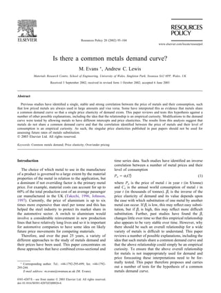
Comparisons with previous results
Fig. 3 contains price and consumption data for the 14
metals mentioned above for the year 1999. Also shown
is the fit given by (3) to this set of data. The full set of
regression results for this year is
ln(Pi) ⫽ 19.953
1.684
11.84
⫺ 0.855ln(Ci)
7.07 t statistic
R2
= 80.48%.
It can be seen that after some 16 years since Georgen-
talis et al. first published their results, there is still a very
strong inverse correlation between metal price and metal
consumption—with some 80.48% of the variation in
metal prices being explained by variations in metals con-
sumption. However, the estimated value for bt appears
to be a little higher than the average value obtained by
Georgentalis et al. Table 1 gives the ln(at) and bt values
obtained for each of the remaining years from 1980 to
1999 (together with their standard errors and R2
values).
As can be seen, and in line with other studies in this
area, they observed very little variation in the value for
bt over time and in fact none of the estimated bt values
were significantly different from each other.
Fig. 4 compares the results shown in Table 1 with the
bt estimates made by Georgentalis et al. It can be seen
that for the overlap years 1980–1983, the current
authors’ estimates for bt are higher than those obtained
by Georgentalis et al. Reasons for this are difficult to
find because the original data used by Georgentalis et
al. are no longer available. It is interesting to note that
a similar observation was made by Jacobson and Evans
when comparing their work to that of Nutting. Recall
that for 1977, Nutting estimated bt to be ⫺0.67, but
Jacobson and Evans found the average value for bt to
Fig. 3. Metal price v. world consumption for 14 metals in 1999.
Table 1
Values obtained by the current authors for the parameters ln(at) and
bt of (3) for the years 1980–1999
Year ln(at) at R2
1980 20.720 (1.478) –0.908 (0.109) 85.26
1981 20.216 (1.409) –0.884 (0.104) 85.74
1982 19.778 (1.421) –0.866 (0.105) 84.89
1983 19.735 (1.569) –0.863 (0.117) 82.05
1984 19.643 (1.535) –0.856 (0.113) 82.62
1985 19.635 (1.542) –0.858 (0.113) 82.66
1986 19.828 (1.619) –0.872 (0.119) 81.74
1987 19.832 (1.712) –0.861 (0.126) 79.65
1988 20.033 (1.731) –0.855 (0.126) 79.24
1989 19.876 (1.653) –0.838 (0.121) 80.12
1990 19.715 (1.672) –0.833 (0.122) 79.55
1991 19.607 (1.680) –0.837 (0.123) 79.47
1992 19.520 (1.730) –0.834 (0.127) 78.33
1993 19.527 (1.803) –0.843 (0.132) 77.27
1994 19.714 (1.809) –0.846 (0.132) 77.40
1995 20.027 (1.716) –0.853 (0.125) 79.64
1996 19.945 (1.682) –0.848 (0.122) 80.05
1997 19.990 (1.653) –0.848 (0.120) 80.76
1998 20.220 (1.577) –0.870 (0.114) 82.94
1999 19.953 (1.684) –0.855 (0.121) 80.48
1980–1999 19.876 (1.633) –0.856 (0.120)
(mean)
R2
is the coefficient of determination measuring the percentage vari-
ation in ln(Pit) explained by variations in ln(Cit). Standard errors are
shown in parentheses.
be closer to ⫺0.74 over the period 1961–1980. Having
said that, when the two sets of bt values are plotted
alongside their respective and approximate 95% confi-
dence intervals, as in Fig. 4, it becomes clear that the
observed differences are not statistically significant. That
is, the confidence intervals for the two separate estimates
of bt over the period 1980–1983 overlap and so there is
not enough evidence to conclude that these two estimates
are actually different.
Results of testing for a common metals demand curve
using over- and underpricing
Fig. 5 shows the extent of over- and underpricing
assuming a common metals demand curve. Under such
an assumption, a metal is said to be overpriced when its
price is consistently in excess of
ln(Pit) ⫽ ln(at) ⫹ btln(Cit),
and underpriced when it is consistently below such a
price. In Fig. 5, the percentage difference between a met-
als actual price and that given by (3) is plotted against
time. The values for at and bt in (3) that are used for
such calculations in each year are those shown in
Table 1.
If the assumption of a common metals demand curve

101
Fig. 4. Values for βt as obtained by Goergentalis et al. for the period 1975–1983 and by present authors for 1980–1999.
Fig. 5. (a) Extent of overpricing for aluminium, copper, iron and gold assuming a common metals demand curve. (b) Extent of overpricing for
nickel, zinc, silver and platinum assuming a common metals demand curve. (c) Extent of overpricing for titanium, vanadium, niobium and chromium
assuming a common metals demand curve. (d) Extent of overpricing for tin and lead assuming a common metals demand curve.
is correct, then the prices given by (3) can be interpreted
as market clearing prices. Overpricing then corresponds
to excess supply and underpricing, excess demand. Fig.
5a,c shows that the metals aluminium, copper, iron and
gold are all “overpriced” to a considerable extent for the
whole length of the sample, whilst the metals titanium,
vanadium, niobium and chromium are “underpriced” to
a considerable extent for the whole length of the sample.
Fig. 5b shows that the metals nickel, zinc, silver and
platinum also remained “overpriced” during the full
length of the sample period but to a lesser extent than
those metals shown in Fig. 5a. Whilst it is believed that
product markets rarely clear instantaneously following a
change in demand or supply conditions, it is highly
unlikely that the prices of all the metals shown in Fig.
5a,c could remain so far away from market clearing lev-
els for such long periods of time. It would therefore
appear that Fig. 5 provides some evidence to suggest
that these metals do not have a common demand curve.
Put differently, the prices given by (3) are not market
clearing prices. Tin and lead remained overpriced for the
first half of the 1980s, but since then have remained mar-
ginally underpriced (Fig. 5d).

Results of testing for a common metals demand curve
using individual demand curves
The first possible generalisation of (3) is to allow each
metals demand curve to have a different intercept value
as in (8). Table 2 shows the result obtained from estimat-
ing (8) using ordinary least squares. Some of the a0i
coefficients were found to be insignificantly different
from zero and so a simplification search procedure was
implemented. Here, the coefficient with the smallest
Student t value was removed and (8) then reestimated.
This procedure was continued until all remaining coef-
ficients were statistically significant at the 5% signifi-
cance level. The results are shown in Table 3. The inter-
cept term of the demand curve for aluminium is
a01 ⫽ 5.5167,
whilst the intercept term of the demand curve for iron
ore (i = 7) is
a01 ⫹ a07 ⫽ 5.5167⫺2.6619 ⫽ 2.8548.
Under this specification, the iron ore demand curve is
parallel to the aluminium demand curve but lies signifi-
cantly below it. Table 4 shows the estimated demand
curves for the remaining metals. It can be seen from this
table that the demand curves for copper, nickel, gold,
silver and platinum lie above that for aluminium, with
the remaining metals having demand curves lying below
that for aluminium.
The Student t values in Table 2 suggest that only two
metals share a common intercept—aluminium and tin
(metal i = 1 and i = 5). This may again be an empirical
curiosity or it may reflect the competition between alu-
minium and tin plate in the packaging sector. All the
Table 2
Ordinary least squares estimate of the coefficients of (8)
Metal Coefficient Estimated value t-value
Aluminium a01 5.2460 1.38
Copper a02 0.1344 0.81
Lead a03 –1.3618 –3.46∗
Nickel a04 0.3985 0.40
Tin a05 0.1112 0.08
Zinc a06 –0.7133 –2.23∗
Iron ore a07 –2.7435 –2.54∗
Gold a08 5.8441 2.02∗
Silver a09 2.4755 1.11
Platinum a010 4.8764 1.26
Chromium a011 –3.7918 –7.95∗
Titanium a012 –1.9868 –4.03∗
Vanadium a013 –0.8264 –0.41
Niobium a014 –0.7916 –0.35
– a1 –0.2781 –4.34∗
– a2 1.9998 2.49∗
– b –0.3554 –1.11
∗
Coefficient significant at the 5% significance level.
Table 3
Ordinary least squares estimate of the simplified version of (8)
Aluminium a01 5.5167 2.23∗
Copper a02 0.1204 10.2∗
Lead a03 –1.3932 –199.0∗
Nickel a04 0.3209 54.0∗
Tin a05
a a
Zinc a06 –0.7391 –86.0∗
Iron ore a07 –2.6619 –69.2∗
Gold a08 5.6207 121.0∗
Silver a09 2.3028 71.1∗
Platinum a010 4.5789 68.2∗
Chromium a011 –3.8296 –729.0∗
Titanium a012 –2.0259 –413.0∗
Vanadium a013 –0.9877 –35.8∗
Niobium a014 –0.9657 –29.5∗
– a1 –0.2790 –4.49∗
– a2 2.0324 3.41∗
– b –0.3801 –55.4∗
∗
a
Coefficient constrained to zero.
Table 4
Estimated individual metals demand curves under specification (8)
Metal Intercept, a1 a2 b
a0i
Aluminiuma
5.5167 –0.2791 2.0324 –0.3801
Copper 5.6371 –0.2791 2.0324 –0.3801
Lead 4.1235 –0.2791 2.0324 –0.3801
Nickel 5.8376 –0.2791 2.0324 –0.3801
Tina
5.5167 –0.2791 2.0324 –0.3801
Zinc 4.7776 –0.2791 2.0324 –0.3801
Iron ore 2.8548 –0.2791 2.0324 –0.3801
Gold 11.1374 –0.2791 2.0324 –0.3801
Silver 7.8195 –0.2791 2.0324 –0.3801
Platinum 10.0956 –0.2791 2.0324 –0.3801
Chromium 1.6871 –0.2791 2.0324 –0.3801
Titanium 3.4908 –0.2791 2.0324 –0.3801
Vanadium 4.5356 –0.2791 2.0324 -0.3801
Niobium 4.5510 –0.2791 2.0324 –0.3801
a1: coefficient in front of variable lnP̄ in (8), a2: coefficient in front
of variable lnĪ in (8), b: coefficient in front of variable lnC in (8).
a
Common metals demand curve.
remaining metals however have an intercept term that
differs significantly to that associated with the metal alu-
minium and so it is clear that most of the 14 metals
studied here do not share a common demand curve.
The next possible generalisation of (3) is to allow each
metal demand curve to have a different slopes or price
elasticity of demand as in (9). Table 5 shows the result
obtained from estimating (9) using ordinary least
squares. Some of the bi coefficients were found to be
insignificantly different from zero and so the above-men-
tioned simplification search procedure was implemented.

103
Table 5
Ordinary least squares estimate of the coefficients of (9)
Aluminium b1 –0.6554 –12.3∗
Copper b2 –0.0013 –0.23
Lead b3 –0.1117 –16.0∗
Nickel b4 –0.0390 –2.88∗
Tin b5 –0.0987 –4.90∗
Zinc b6 –0.0643 –9.94∗
Iron ore b7 –0.0865 –8.49∗
Gold b8 0.4067 6.48∗
Silver b9 0.0391 1.01
Platinum b10 0.2702 1.98∗
Chromium b11 –0.2781 –36.3∗
Titanium b12 –0.1611 –20.7∗
Vanadium b13 –0.2565 –7.92∗
Niobium b14 –0.2978 –7.61∗
– a0 8.1256 4.02∗
– a1 –0.3185 –3.95∗
– a2 2.5084 4.89∗
∗
The results are shown in Table 6. The inverse of the
price elasticity of the demand for aluminium is
b1 ⫽ ⫺0.6524,
whilst the inverse of the price elasticity of demand for
iron ore (i = 7) is
b1 ⫹ b7 ⫽ ⫺0.6524⫺0.0865 ⫽ ⫺0.7389.
Aluminium is therefore more price elastic than iron
Table 6
Ordinary least squares estimate of the simplified version of (9)
Aluminium b1 –0.6524 –12.6∗
Copper b2
a a
Lead b3 –0.1108 –18.9∗
Nickel b4 –0.0376 –3.12∗
Tin b5 –0.0968 –5.28∗
Zinc b6 –0.0635 –11.7∗
Iron ore b7 –0.0865 –8.51∗
Gold b8 0.4115 6.98∗
Silver b9 0.0423 1.98∗
Platinum b10 0.2800 2.17∗
Chromium b11 –0.2771 –42.8∗
Titanium b12 –0.1602 –24.3∗
Vanadium b13 –0.2537 –8.44∗
Niobium b14 –0.2946 –8.07∗
– a0 8.0962 4.02∗
– a1 –0.3185 –3.96∗
– a2 2.5014 4.89∗
∗
a
Coefficient constrained to zero.
ore. Table 7 shows the estimated demand curves for the
remaining metals. It can be seen from this table that the
metals gold, silver and platinum are more price elastic
than aluminium and the metals lead, nickel, tin, zinc,
iron ore, chrome, titanium, vanadium and niobium are
less price elastic than aluminium.
The Student t values in Table 5 suggest that two met-
als appear to share a common price elasticity of
demand—aluminium and copper (metal i = 1 and i =
2). This may reflect the competition between aluminium
and copper in the transport sector (which was around
15% of the copper market in 1994) and the electronics
sector (which accounted for around 25% of the markets
for copper). All the remaining metals however have price
elasticities that differ significantly to that associated with
the metal aluminium and so it is clear that most of the
14 metals studied do not share a common demand curve.
It would appear that most metals have demand curves
with differing slopes—as in Fig. 2—so that (3) depicts
the mongrel function that is neither a supply nor a
demand curve. Yet Table 7 reveals that most metals have
a similar, but statistically different price elasticity of
demand. Gold and platinum appear to be more price
elastic than most, whilst niobium, vanadium and chro-
mium are more price inelastic than most. The remaining
nine metals have inverse price elasticities close to 0.7.
This is a lot lower than the bt values shown in Table 1,
and so it would be dangerous to use such values to infer
something on rates of future substitution between metals.
The final generalisation of (3) to be considered in this
paper is to allow each metal demand curve to have a
different slopes or price elasticities of demand and dif-
ferent intercepts as in (10). However, the results obtained
for such a generalisation were not satisfactory. Table 8
shows the simplified estimated demand curve for each
Table 7
Metal Intercept, a0 a1 a2 bi
Aluminiuma
8.0962 –0.3185 2.5014 –0.6524
Coppera
8.0962 –0.3185 2.5014 –0.6524
Lead 8.0962 –0.3185 2.5014 –0.7632
Nickel 8.0962 –0.3185 2.5014 –0.6900
Tin 8.0962 –0.3185 2.5014 –0.7492
Zinc 8.0962 –0.3185 2.5014 –0.7159
Iron ore 8.0962 –0.3185 2.5014 –0.7389
Gold 8.0962 –0.3185 2.5014 –0.2409
Silver 8.0962 –0.3185 2.5014 –0.6101
Platinum 8.0962 –0.3185 2.5014 –0.3724
Chromium 8.0962 –0.3185 2.5014 –0.9295
Titanium 8.0962 –0.3185 2.5014 –0.8126
Vanadium 8.0962 –0.3185 2.5014 –0.9061
Niobium 8.0962 –0.3185 2.5014 –0.9470
a
Common metals demand curve.

Table 8
Metal Intercept, a0i a1 a2 bi
Aluminium 18.7485 –0.2647 2.0096 –1.1687
Coppera
18.5024 –0.2647 2.0096 –1.1687
Leadb
18.7485 –0.2647 2.0096 –1.1687
Nickel –3.5515 –0.2647 2.0096 0.3134
Tinc
18.7485 –0.2647 2.0096 –1.4508
Zinc –11.1567 –0.2647 2.0096 0.6362
Iron oreb
18.7485 –0.2647 2.0096 –1.1687
Gold 11.4154 –0.2647 2.0096 –1.9277
Silvera
15.5736 –0.2647 2.0096 –1.1687
Platinum 9.6025 –0.2647 2.0096 –0.2649
Chromium –1.0923 –0.2647 2.0096 –0.1944
Titanium –13.1410 –0.2647 2.0096 1.4497
Vanadium 4.8748 –0.2647 2.0096 1.3043
Niobium 16.3934 –0.2647 2.0096 –0.4083
a
Common price elasticity with aluminium.
b
Common intercept and price elasticity with aluminium.
c
Common intercept with aluminium.
metal under this specification and as can be seen, four
of the metals appear to have a positive price elasticity
of demand—nickel, zinc, titanium and vanadium.
Conclusions
A number of conclusions can be drawn from the above
study. First, the empirical correlation between a metals
price and its level of consumption first identified by
Hughes in 1972 still holds today, with roughly the same
price elasticity of demand. However, this relationship
should be interpreted as mongrel function rather than as
a stable common metals demand curve. The stability
over time probably reflects the fact that the same type
of information is being averaged each year. As such, the
singular price elasticities published in past papers should
not be used for assessing future rates of metals substi-
tution.
Secondly, when price elasticities are allowed to vary
between metals, the resulting estimates suggest that met-
als have similar but statistically different rates of substi-
tution. Platinum and gold have the highest rates of sub-
stitution whilst niobium and chrome have the lowest
rates of substitution. Finally, it appears to be the case
that aluminium and copper share a common price elas-
ticity of demand and this is consistent with the fact that
these metals compete in some of their major markets.
References
Balestra, P., Nerlove, M., 1966. Pooling cross-section and time-series
data in the estimation of a dynamic model: the demand for natural
gas. Econometrica 34, 585–612.
Bozdogan, K., Hartmnn, R.S., 1979. US demand for copper: an intro-
duction to theoretical and econometric analysis. In: Mikesell, R.F.
(Ed.), The World Copper Industry. The Johns Hopkins University
Press for Resources for the Future, Baltimore, MD, pp. 131–163.
Evans, M., 1996. Modelling steel demand in the UK. Ironmaking and
Steelmaking 23, 17–24.
Figuerola-Ferretti, I., Gilbert, C.L., 2001. Price variability and market-
ing method in non-ferrous metals: Slade’s analysis revisited.
Resources Policy 27, 169–177.
Georgentalis, S., Nutting, J., Phillips, G., 1990. Relationship between
price and consumption of metals. Materials Science and Tech-
nology 6, 192–195.
Hughes, J.E., 1972. The exploitation of metals. Metals and Materials
May, 197–205.
International Financial Statistics Yearbook (1980–1989). International
Monetary Fund Publications, Washington, DC, Table Z.
Jacobson, D.M., Evans, D.S., 1985. The price of metals. Materials and
Society 9, 331–347.
Johnson, R., 1997. VW climbs back into the drivers seat. Automotive
News Europe April, 8.
Labson, B.S., Crompton, P.L., 1993. Common trends in economic
activity: cointegration and the intensity of use debate. Journal of
Environmental Economics and Management 25, 147–161.
MacAvoy, P.W., 1988. Explaining Metal Prices. Kluwer Academic
Publishers, London.
Maddala, G.S., 2001. Introduction to Econometrics. John Wiley &
Sons, New York Chapter 15, pp. 573–583.
Metals Bulletin (1980–1989). Mining Journal Books Ltd, Eden-
bridge, Kent.
Minerals Handbook (1980–1989). American Metal Market, New York.
Myers, J.G., 1986. Testing for structural change in metal use. Materials
and Society, 271–283.
Nutting, J., 1977. Metals as materials. Metals and Materials
July/August, 30–34.
Platinum (1980–1989). Johnson Matthey, London.
Slade, M.E., 1981. Recent advances in econometric estimation of
materials substitution. Resources Policy 7, 103–109.
Takechi, H., 1996. Lighter vehicle weight and steel materials. Steel
Today and Tomorrow January, 5–8.
Tilton, J.E., 1990. World Metal Demand: Trends and Prospects.
Resources for the Future, Washington, DC pp. 25–30.
Tilton, J.E., Fanyu, P., 1999. Consumer preferences, technological
change, and the short run income elasticity of demand. Resources
Policy 25, 87–109.
Tilton, J.E., Moore, D.J., Shields, D.J., 1996. Economic growth and the
demand for construction materials. Resources Policy 22, 197–205.
Valdes, R.M., 1990. Modelling Australian steel consumption: the
intensity of use technique. Resource Policy 16, 172–183.

foro 1.pdf

Recommended

Recommended

More Related Content

Similar to foro 1.pdf

Similar to foro 1.pdf (20)

Recently uploaded

Recently uploaded (16)

foro 1.pdf