Axial Deformation's Role in Rigidly Fixed Portal Frame Analysis

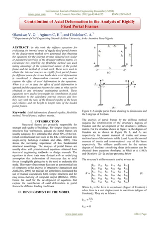
International Journal of Modern Engineering Research (IJMER)
www.ijmer.com Vol.2, Issue.6, Nov-Dec. 2012 pp-4244-4255 ISSN: 2249-6645

Contribution of Axial Deformation in the Analysis of Rigidly
Fixed Portal Frames
Okonkwo V. O.1, Aginam C. H.2, and Chidolue C. A.3
123
Department of Civil Engineering Nnamdi Azikiwe University, Awka Anambra State-Nigeria

ABSTRACT: In this work the stiffness equations for
evaluating the internal stress of rigidly fixed portal frames
by the displacement method were generated. But obtaining
the equations for the internal stresses required non-scalar
or parametric inversion of the structure stiffness matrix. To
circumvent this problem, the flexibility method was used
taking advantage of the symmetrical nature of the portal
frame and the method of virtual work. These were used to
obtain the internal stresses on rigidly fixed portal frames
for different cases of external loads when axial deformation
is considered. A dimensionless constant s was used to
capture the effect of axial deformation in the equations.
When it is set to zero, the effect of axial deformation is
ignored and the equations become the same as what can be
obtained in any structural engineering textbook. These
equations were used to investigate the contribution of axial
deformation to the calculated internal stresses and how
they vary with the ratio of the flexural rigidity of the beam
and columns and the height to length ratio of the loaded
portal frames.
Figure 1: A simple portal frame showing its dimensions and
Keywords: Axial deformation, flexural rigidity, flexibility
the 6 degrees of freedom
method, Portal frames, stiffness matrix,
The analysis of portal frames by the stiffness method
I. INTRODUCTION requires the determination of the structure’s degrees of
Structural frames are primarily responsible for
freedom and the development of the structure’s stiffness
strength and rigidity of buildings. For simpler single storey
matrix. For the structure shown in Figure 1a, the degrees of
structures like warehouses, garages etc portal frames are
freedom are as shown in Figure 1b. I1 and A1 are
usually adequate. It is estimated that about 50% of the hot- respectively the second moment of inertia and cross-
rolled constructional steel used in the UK is fabricated into sectional area of the columns while I2 and A2 are the second
single-storey buildings (Graham and Alan, 2007). This moment of inertia and cross-sectional area of the beam
shows the increasing importance of this fundamental
respectively. The stiffness coefficients for the various
structural assemblage. The analysis of portal frames are
degrees of freedom considering shear deformation can be
usually done with predetermined equations obtained from obtained from equations developed in Ghali et al (1985)
structural engineering textbooks or design manuals. The
and Okonkwo (2012) and are presented below
equations in these texts were derived with an underlying
assumption that deformation of structures due to axial The structure’s stiffness matrix can be written as:
forces is negligible giving rise to the need to undertake this
study. The twenty first century has seen an astronomical use 𝑘11 𝑘12 𝑘13 𝑘14 𝑘15 𝑘16
of computers in the analysis of structures (Samuelsson and 𝑘21 𝑘22 𝑘23 𝑘24 𝑘25 𝑘26
Zienkiewi, 2006) but this has not completely eliminated the 𝑘 𝑘32 𝑘33 𝑘34 𝑘35 𝑘36
use of manual calculations form simple structures and for 𝐾 = 31 . (1)
𝑘41 𝑘42 𝑘43 𝑘44 𝑘45 𝑘46
easy cross-checking of computer output (Hibbeler, 2006). 𝑘51 𝑘52 𝑘53 𝑘54 𝑘55 𝑘56
Hence the need for the development of equations that 𝑘61 𝑘62 𝑘63 𝑘64 𝑘65 𝑘66
capture the contribution of axial deformation in portal
frames for different loading conditions. Where kij is the force in coordinate (degree of freedom) i
when there is a unit displacement in coordinate (degree of
II. DEVELOPMENT OF THE MODEL freedom) j. They are as follows:
𝐸𝐴1
𝑘11 = ℎ

𝑘12 = 0

www.ijmer.com 4244 | Page

6𝐸𝐼2 𝑑1
𝑘13 = 𝑙2
𝑑2
12𝐸𝐼1 𝑑3
𝑘14 = − ℎ3
{𝐷} = . . . . . (5)
𝑑4
𝑑5
𝑘15 = 0
𝑑6
6𝐸𝐼2
𝑘16 = 𝑙2 Where di is the displacement in coordinate i.
12𝐸𝐼1 𝐸𝐴2 𝐹1
𝑘22 = ℎ3
+ 𝑙
𝐹2
6𝐸𝐼1 𝐹3
𝑘23 = {𝐹} = . . . . . . (6)
ℎ2 𝐹4
𝐹5
𝑘24 = 0
𝐹6
𝐸𝐴2
𝑘25 = − 𝑙
. . (2) Where Fi is the external load with a direction coinciding
with the coordinate i (McGuire et al, 2000).
𝑘26 = 0
By making {D} the subject of the formula in equation (3)
4𝐸𝐼2 4𝐸𝐼1
𝑘33 = +
𝑙 ℎ −1
𝐷 = 𝐾 {𝐹 − 𝐹𝑜 } . . . . (7)
6𝐸𝐼2
𝑘34 = − 𝑙2 Once {D} is obtained the internal stresses in the frame can
be easily obtained by writing the structure’s compatibility
𝑘35 = 0 equations given as
2𝐸𝐼2
𝑘36 = 𝑙
𝑀 = 𝑀 𝑟 + 𝑀1 𝑑1 + 𝑀2 𝑑2 + 𝑀3 𝑑3 . . (8)

12𝐸𝐼2 𝐸𝐴1 Where M is the internal stress (bending moment) at any
𝑘44 = +
𝑙3 ℎ point on the frame, Mr is the internal stress at the point
under consideration in the restrained structure while Mi is
𝑘45 = 0 the internal stress at the point when there is a unit
6𝐸𝐼2 displacement in coordinate i.
𝑘46 = − To solve equation (8) there is need to obtain {D}. {D} can
𝑙2
be obtained from the inversion of [K] in equation (7).
12𝐸𝐼1 𝐸𝐴2
𝑘55 = + Finding the inverse of K parametrically (i.e. without
ℎ3 𝑙
substituting the numerical values of E, h, l etc) is a difficult
From Maxwell’s Reciprocal theorem and Betti’s Law k ij = task. This problem is circumvented by using the flexibility
kji ( Leet and Uang, 2002). method to solve the same problem, taking advantage of the
symmetrical nature of the structure and the principle of
When there are external loads on the structure on the virtual work.
structure there is need to calculate the forces in the
restrained structure Fo as a result of the external load. III. APPLICATION OF THE FLEXIBILITY
MODEL
The structure’s equilibrium equations are then written as The basic system or primary structure for the structure in
Figure 1a is given in Figure 2. The removed redundant
{𝐹} = {𝐹𝑜 } + 𝐾 {𝐷} . . . . (3) force is depicted with X1.
𝑘10
𝑘20
𝑘30
{𝐹𝑜 } = . . . . . (4)
𝑘40
𝑘50
𝑘60

Where kio is the force due to external load in coordinate i
when the other degrees of freedom are restrained.

Figure 2: The Basic System showing the removed
redundant forces


The flexibility matrix of the structure can be determined 1 12𝐸𝐼1 𝐼2 𝐴1
= . . . (15a)
𝑑 11 𝐼1 𝐴1 𝑙 3 +6𝐼2 𝐴1 𝑙 2 ℎ +24𝐼1 𝐼2 ℎ
using the principle of virtual work.
By applying the unit load theorem the deflection in beams
or frames can be determined for the combined action of the
internal stresses, bending moment and axial forces with 𝑑 33 3𝐸𝐼1 𝐴2 (𝑙𝐼1 +2ℎ𝐼2 )
𝑀 𝑀 𝑁 𝑁 2
𝑑 22 𝑑 33 −𝑑 23
= 2𝐴 3 2 2 4 . (15b)
𝐷= 𝑑𝑠 + 𝑑𝑠 . . . (9) 2 ℎ 𝑙𝐼1 +3𝐼1 𝑙 +𝐴2 ℎ 𝐼2 +6ℎ𝑙𝐼1 𝐼2
𝐸𝐼 𝐸𝐴
𝑑 32 −3𝐸𝐼1 𝐼2 𝐺𝐴2 ℎ 2
Where 𝑀 and 𝑁 are the virtual internal stresses while M 2
𝑑 22 𝑑 33 −𝑑 23
= 2𝐴 3 2 2 4 (15c)
2 ℎ 𝑙𝐼1 +3𝐼1 𝑙 +𝐴2 ℎ 𝐼2 +6ℎ𝑙𝐼1 𝐼2
and N are the real/actual internal stresses.
𝑑 22 𝐸𝐼1 𝐼2 2𝐴2 ℎ 3 +3𝐼1 𝑙
E is the modulus of elasticity of the structural material 2 = 3 𝑙𝐼 +3𝐼 2 𝑙 2 +𝐴 ℎ 4 𝐼 +6ℎ𝑙𝐼 𝐼 . (15d)
𝑑 22 𝑑 33 −𝑑 23 2𝐴2 ℎ 1 1 2 2 1 2

A is the cross-sectional area of the element (McGuire et al, Equation (12) is evaluated to get the redundant forces and
2000; Nash, 1998) these are substituted into the structures force equilibrium
(superposition) equations to obtain the internal stresses at
If dij is the deformation in the direction of i due to a unit any point.
load at j then by evaluating equation (9) the following are
obtained: 𝑀 = 𝑀 𝑜 + 𝑀1 𝑋1 + 𝑀2 𝑋2 + 𝑀3 𝑋3 . . (16)
𝐼1 𝐺𝐴1 𝑙 3 +6𝐼2 𝐴1 𝑙 2 ℎ +12𝐼1 𝐼2 ℎ Where M is the required stress at a point, Mo is the stress at
𝑑11 = . . (10a)
12𝐸𝐼1 𝐼2 𝐴1 that point for the reduced structure, Mi is stress at that point
when the only the redundant force Xi =1 acts on the reduced
𝑑12 = 0 . . . . . (10b) structure.
For the loaded portal frame of Figure 3, the deformations of
𝑑13 = 0 . . . . . . (10c)
the reduced structure due to external loads are
2𝐴2 ℎ 3 +3𝐼1 𝑙
𝑑22 = 3𝐸𝐼1 𝐴2
. . . (10d) 𝑑10 = 0 . . . . .
. (17a)
−ℎ 2
𝑑23 = 𝐸𝐼1
. . . (10e) 𝑤 ℎ 2 𝑙2
𝑑20 = . . . . .
8𝐸𝐼1
𝑙𝐼1 +2ℎ 𝐼2 . (17b)
𝑑33 = . . . . (10f)
𝐸𝐼1 𝐼2
−𝑤 𝑙 2 (𝑙𝐼1 +6ℎ𝐼2 )
From Maxwell’s Reciprocal theorem and Betti’s Law dij = 𝑑30 = . . (17c)
24𝐸𝐼1 𝐼2
dji.
By substituting the values of equations (17a) – (17c) into
The structure’s compatibility equations can be written thus equations (12)

𝑑11 𝑑11 𝑑11 𝑋1 𝑑10 𝑋1 = 0 . . . . . (18a)
𝑑21 𝑑21 𝑑21 𝑋2 + 𝑑20 = 0 . (11a)
𝑑31 𝑑31 𝑑31 𝑋3 𝑑30 −𝐴2 𝐼1 𝑤ℎ 2 𝑙 3
𝑋2 = 4 2
2𝐴2 ℎ 3 𝑙𝐼1 +3𝐼1 𝑙 2 +𝐴2 ℎ 4 𝐼2 +6ℎ𝑙𝐼1 𝐼2
. (18b)
i.e. 𝑓𝐹 + 𝑑 𝑜 = 0 . . . (11b) 2
𝑤 𝑙 2 2𝐴2 ℎ 3 𝑙𝐼1 +3𝐼1 𝑙 2 +3𝐴2 ℎ 4 𝐼2 +18ℎ𝑙𝐼1 𝐼2
𝑋3 = 2
24 2𝐴2 ℎ 3 𝑙𝐼1 +3𝐼1 𝑙 2 +𝐴2 ℎ 4 𝐼2 +6ℎ𝑙𝐼1 𝐼2
. (18c)
Where F is the vector of redundant forces X1, X2, X3 and do
is the vector deformation d10, d20, d30 due to external load
Evaluating equation (16) for different points on the
on the basic system (Jenkins, 1990).
structure using the force factors obtained in equations (18a)
𝐹 = 𝑓 −1 (−𝑑 𝑜 ) . . . . (12) – (18c)
2𝑤𝑙 3 𝐼1 ℎ 3 𝐴2 −3𝑙𝐼1
𝑀 𝐴 = 12 2
2𝐴2 ℎ 3 𝑙𝐼1 +3𝐼1 𝑙 2 +𝐴2 ℎ 4 𝐼2 +6ℎ𝑙𝐼1 𝐼2
. . (19)
𝐴𝑑𝑗 𝑓
𝑓 −1 = 𝑑𝑒𝑡 𝑓
. . (13)

−2𝑤𝑙 3 𝐼1 2ℎ 3 𝐴2 +3𝑙𝐼1
(Stroud, 1995) 𝑀 𝐵 = 24 2 . . (20)
2𝐴2 ℎ 3 𝑙𝐼1 +3𝐼1 𝑙 2 +𝐴2 ℎ 4 𝐼2 +6ℎ𝑙𝐼1 𝐼2
1
𝑑 11
0 0
𝑑 33 −𝑑 32
𝑓 −1 = 0 2
𝑑 22 𝑑 33 −𝑑 23 2
𝑑 22 𝑑 33 −𝑑 23 . (14) −2𝑤 𝑙 3 𝐼1 2ℎ 3 𝐴2 +3𝑙𝐼1
𝑀𝐶 = 2 . (21)
−𝑑 23 𝑑 22 24 2𝐴2 ℎ 3 𝑙𝐼1 +3𝐼1 𝑙 2 +𝐴2 ℎ 4 𝐼2 +6ℎ𝑙𝐼1 𝐼2
0 2 2
𝑑 22 𝑑 33 −𝑑 23 𝑑 22 𝑑 33 −𝑑 23
−𝑤 𝑙 3 𝐼1 8𝐼2 ℎ 3 +𝑠2 𝑙 3 𝐼1
𝑀𝐶 =
From equations 10a – 10f 12 4ℎ 3 𝐼2 2𝑙𝐼1 +ℎ 𝐼2 +𝑠2 𝑙 3 𝐼1 𝑙𝐼1 +2ℎ 𝐼2


2𝑤𝑙 3 𝐼1 ℎ 3 𝐴2 −3𝑙𝐼1 −𝑤 ℎ 3
𝑀𝐷 = 2 . . (22) 𝑑30 = . . . . . (30c)
12 2𝐴2 ℎ 3 𝑙𝐼1 +3𝐼1 𝑙 2 +𝐴2 ℎ 4 𝐼2 +6ℎ𝑙𝐼1 𝐼2 6𝐸𝐼1

equations (12)
the reduced structure due to external loads are 𝑤 ℎ 3 𝑙𝐼2 𝐴1
𝑋1 = 𝐼1 𝐴1 𝑙 3 +6𝐼2 𝐴1 𝑙 2 ℎ +24ℎ 𝐼1 𝐼2
. . . (31a)
−𝑤𝑙 𝑙 3 𝐼1 𝐴1 +8ℎ 𝑙 2 𝐼2 𝐴1 +64ℎ 𝐼1 𝐼2
𝑑10 = . (23a) −𝑤ℎ 4 𝐴2 3𝑙𝐼1 +2ℎ 𝐼2
128 𝐸𝐼1 𝐼2 𝐴1 𝑋2 = 8 3 𝑙𝐼 +3𝐼 2 𝑙 2 +𝐴 ℎ 4 𝐼 +6ℎ𝑙𝐼 𝐼
2𝐴2 ℎ 1
. (31b)
1 2 2 1 2
𝑤 ℎ 2 𝑙2
𝑑20 = 16𝐸𝐼1
. . . (23b) 𝑤ℎ 3 𝐼2 −ℎ 3 𝐴2 +12𝑙𝐼1
𝑋3 = 24 2
2𝐴2 ℎ 3 𝑙𝐼1 +3𝐼1 𝑙 2 +𝐴2 ℎ 4 𝐼2 +6ℎ𝑙𝐼1 𝐼2
. . (31c)
−𝑤 𝑙 2 (𝑙𝐼1 +6ℎ𝐼2 )
𝑑30 = . . (23c) Evaluating equation (16) for different points on the
48𝐸𝐼1 𝐼2
By substituting the values of equations (23a) – (23c) into – (31c)
equations (12)
𝑀𝐴 =
3𝑤𝑙 𝑙 3 𝐼1 𝐴1 +8ℎ 𝑙 2 𝐼2 𝐴1 +64ℎ𝐼1 𝐼2 𝑤 ℎ 2 𝐼1 𝐴1 𝑙 3 +5𝐴1 𝑙 2 ℎ 𝐼2 +24ℎ𝐸𝐼1 𝐼2
𝑋1 = . . (24a) − +
32 𝐼1 𝐴1 𝑙 3 +6𝐼2 𝐴1 𝑙 2 ℎ +24ℎ 𝐼1 𝐼2 2 𝐼1 𝐴1 𝑙 3 +6𝐼2 𝐴1 𝑙 2 ℎ +24ℎ 𝐼1 𝐼2
𝑤 ℎ 3 9ℎ 2 𝑙𝐼1 𝐴2 +5𝐴2 ℎ 3 𝐼2 +12𝑙𝐼1 𝐼2
−2𝑤 ℎ 2 𝑙 3 𝐴2 𝐼1 2 . . . . (32)
𝑋2 = 16 . (24b) 24 2𝐴2 ℎ 3 𝑙𝐼1 +3𝐼1 𝑙 2 +𝐴2 ℎ 4 𝐼2 +6ℎ𝑙𝐼1 𝐼2
2
2𝐴2 ℎ 3 𝑙𝐼1 +3𝐼1 𝑙 2 +𝐴2 ℎ 4 𝐼2 +6ℎ𝑙𝐼1 𝐼2

𝑤 ℎ 3 𝑙 2 𝐴2 3ℎ 𝐼2 +2𝑙𝐼1 +3𝑤𝑙 3 𝐼1 𝑙𝐼1 +6ℎ 𝐼2
𝑋3 = 2 . (24c) 𝑀𝐵 =
48 2𝐴2 ℎ 3 𝑙𝐼1 +3𝐼1 𝑙 2 +𝐴2 ℎ 4 𝐼2 +6ℎ𝑙𝐼1 𝐼2
𝑤 ℎ 3 𝑙 2 𝐼2 𝐴1 𝑤ℎ 3 𝐼2 −ℎ 3 𝐴2 +12𝑙𝐼1
3 +6𝐼 𝐴 𝑙 2 ℎ +24ℎ 𝐼 𝐼 + 24 3 𝑙𝐼 +3𝐼 2 𝑙 2 +𝐴 ℎ 4 𝐼 +6ℎ𝑙𝐼 𝐼 .
𝑠2 2 𝐼1 𝐴1 𝑙 2 1 1 2 2𝐴2 ℎ 1 1 2 2 1 2
Let 𝛽 = . . . . . . (25) . . (33)
𝑠1

Evaluating equation (16) for different points on the 𝑀𝐶 =
structure using the force factors obtained in equations (24a) 𝑤 ℎ 3 𝑙 2 𝐼2 𝐴1 𝑤ℎ 3 𝐼2 −ℎ 3 𝐴2 +12𝑙𝐼1
−2 + 24
– (24c) 𝐼1 𝐴1 𝑙 3 +6𝐼2 𝐴1 𝑙 2 ℎ +24ℎ𝐼1 𝐼2 2
2𝐴2 ℎ 3 𝑙𝐼1 +3𝐼1 𝑙 2 +𝐴2 ℎ 4 𝐼2 +6ℎ𝑙𝐼1 𝐼2
. . . . (34)
𝑀𝐴 =
𝑤 𝑙 2 ℎ 3 𝐴2 3ℎ 𝐼2 +8𝑙𝐼1 +3𝑙𝐼1 𝑙𝐼1 +6ℎ𝐼2 𝑤 𝑙 4 𝐴1 5𝑙𝐼1 +24ℎ 𝐼2 𝑀𝐷 =
2 − 64 𝑤 ℎ 3 𝑙 2 𝐼2 𝐴1 𝑤ℎ 3 9ℎ 2 𝑙𝐼1 𝐴2 +5𝐴2 ℎ 3 𝐼2 +12𝑙𝐼1 𝐼2
48 2𝐴2 ℎ 3 𝑙𝐼1 +3𝐼1 𝑙 2 +𝐴2 ℎ 4 𝐼2 +6ℎ𝑙𝐼1 𝐼2 𝐼1 𝐴1 𝑙 3 +6𝐼2 𝐴1 𝑙 2 ℎ +24ℎ𝐼1 𝐼2
−2 3 +6𝐼 𝐴 𝑙 2 ℎ +24ℎ𝐼 𝐼 + 24 2
. . . . (26) 𝐼1 𝐴1 𝑙 2 1 1 2 2𝐴2 ℎ 3 𝑙𝐼1 +3𝐼1 𝑙 2 +𝐴2 ℎ 4 𝐼2 +6ℎ𝑙𝐼1 𝐼2
. . . . (35)
𝑀𝐵 =
𝑤 𝑙 4 𝐴1 5𝑙𝐼1 +24ℎ 𝐼2 For the loaded portal frame of Figure 6, the deformations of
− 64 𝐼1 𝐴1 𝑙 3 +6𝐼2 𝐴1 𝑙 2 ℎ +24ℎ 𝐼1 𝐼2
+
𝑤 𝑙 2 ℎ 3 𝐴2 3ℎ 𝐼2 +2𝑙𝐼1 +3𝑙𝐼1 𝑙𝐼1 +6ℎ𝐼2
2 . . . (27)
48 2𝐴2 ℎ 3 𝑙𝐼1 +3𝐼1 𝑙 2 +𝐴2 ℎ 4 𝐼2 +6ℎ𝑙𝐼1 𝐼2 𝑃𝑎 2 𝑙
𝑑10 = − . . . (36a)
2𝐸𝐼1
𝑀𝐶 =
3𝑤 𝑙 2 𝑙 3 𝐼1 𝐴1 +8ℎ 𝑙 2 𝐼2 𝐴1 +64ℎ𝐼1 𝐼2 𝑑20 = 0 . . . . (36b)
− +
64 𝐼1 𝐴1 𝑙 3 +6𝐼2 𝐴1 𝑙 2 ℎ +24ℎ 𝐼1 𝐼2
𝑤 𝑙 2 ℎ 3 𝐴2 3ℎ 𝐼2 +2𝑙𝐼1 +3𝑙𝐼1 𝑙𝐼1 +6ℎ𝐼2 𝑑30 = 0 . . . (36c)
2
48 2𝐴2 ℎ 3 𝑙𝐼1 +3𝐼1 𝑙 2 +𝐴2 ℎ 4 𝐼2 +6ℎ𝑙𝐼1 𝐼2
. . . (28)
equations (12)
𝑀𝐷 = 6𝑃𝑎 2 𝑙𝐼2 𝐴1
3𝑤 𝑙 2 𝑙 3 𝐼1 𝐴1 +8ℎ 𝑙 2 𝐼2 𝐴1 +64ℎ𝐼1 𝐼2
𝑋1 = 𝐴1 𝐼1 𝑙 3 +6𝐴1 ℎ 𝑙 2 𝐼2 +24ℎ 𝐼1 𝐼2
. . . (37a)
− 64 𝐼1 𝐴1 𝑙 3 +6𝐼2 𝐴1 𝑙 2 ℎ +24ℎ 𝐼1 𝐼2
+
𝑤 𝑙 2 ℎ 3 𝐴2 3ℎ 𝐼2 +8𝑙𝐼1 +3𝑙𝐼1 𝑙𝐼1 +6ℎ𝐼2 𝑋2 = 0 . . . . (37b)
2
48 2𝐴2 ℎ 3 𝑙𝐼1 +3𝐼1 𝑙 2 +𝐴2 ℎ 4 𝐼2 +6ℎ𝑙𝐼1 𝐼2
. . . (29)
𝑋3 = 0 . . . . . . (37c)
the reduced structure due to external loads are Evaluating equation (16) for different points on the
𝑤𝑙 ℎ 3
𝑑10 = − . . . . (30a) – (37c)
12𝐸𝐼1

𝑤ℎ4
𝑑20 = . . . . (30b)
8𝐸𝐼1


3𝑎𝑙 2 𝐼2 𝐴1 For the loaded portal frame of Figure 8, the deformations of
𝑀 𝐴 = −𝑃𝑎 1 − 𝐴1 𝐼1 𝑙 3 +6𝐴1 ℎ 𝑙 2 𝐼2 +24ℎ 𝐼1 𝐼2
. (38)
3𝑃𝑎 2 𝑙 2 𝐼2 𝐴1 𝑎 2 𝐼1 𝐴1 3𝑙 −2𝑎 +6ℎ 𝐼2 𝑎𝑙 𝐴1 +2𝐼1
𝑀𝐵 = 𝐴1 𝐼1 𝑙 3 +6𝐴 ℎ 𝑙 2 𝐼 +24ℎ 𝐼 𝐼 . . (39) 𝑑10 = −𝑃 . (48a)
1 2 1 2 12𝐸𝐼1 𝐼2 𝐴1

𝑃𝑎ℎ 2
𝑑20 = 2𝐸𝐼1
. . . (48b)
3𝑃𝑎 2 𝑙 2 𝐼2 𝐴1
𝑀𝐶 = − 𝐴1 𝐼1 𝑙 3 +6𝐴1 ℎ 𝑙 2 𝐼2 +24ℎ𝐼1 𝐼2
. . (40) 𝑃𝑎 𝑎𝐼1 +2ℎ 𝐼2
𝑑30 = − . . . (48c)
2𝐸𝐼1 𝐼2
3𝑎𝑙 2 𝐼2 𝐴1
𝑀 𝐷 = 𝑃𝑎 1 − . . (41)
𝐴1 𝐼1 𝑙 3 +6𝐴1 ℎ 𝑙 2 𝐼2 +24ℎ 𝐼1 𝐼2 By substituting the values of equations (48a) – (48c) into
equations (12)

𝑃 𝑎 2 𝐼1 𝐴1 3𝑙−2𝑎 +6ℎ𝐼2 𝑎𝑙 𝐴1 +2𝐼1
For the loaded portal frame of Figure 7, the deformations of 𝑋1 = . (49a)
𝐼1 𝐴1 𝑙 3 +6𝐼2 𝐴1 𝑙 2 ℎ +24ℎ 𝐼1 𝐼2
−3𝑃𝑎 ℎ 2 𝐼1 𝐴2 𝑙−𝑎
𝑃𝑎 2 𝑙 𝑋2 = 2 2
2𝐴2 ℎ 3 𝑙𝐼1 +3𝐼1 𝑙 2 +𝐴2 ℎ 4 𝐼2 +6ℎ𝑙𝐼1 𝐼2
(49b)
𝑑10 = − 4𝐸𝐼 . . . (42a)
1
𝑃𝑎 ℎ 3 𝐴2 2𝑎𝐼1 +ℎ 𝐼2 +3𝑙𝐼1 𝑎𝐼1 +2ℎ 𝐼2
𝑃𝑎 2 3ℎ −𝑎 𝑋3 = 2
2 2𝐴2 ℎ 3 𝑙𝐼1 +3𝐼1 𝑙 2 +𝐴2 ℎ 4 𝐼2 +6ℎ𝑙𝐼1 𝐼2
(49c)
𝑑20 = . . (42b)
6𝐸𝐼1

𝑃𝑎 2
𝑑30 = − 2𝐸𝐼 . . . . (42c)
1
Evaluating equation (16) for different points on the
By substituting the values of equations (42a) – (42c) into structure using the force factors obtained in equations (49a)
equations (12) – (49c)

3𝑃𝑎 2 𝑙𝐼2 𝐴1 𝑃𝑙 𝑎 2 𝐼1 𝐴1 3𝑙−2𝑎 +6ℎ 𝐼2 𝑎𝑙 𝐴1 +2𝐼1
𝑋1 = . . . (43a) 𝑀 𝐴 = −𝑃𝑎 + +
𝐼1 𝐴1 𝑙 3 +6𝐼2 𝐴1 𝑙 2 ℎ +24ℎ 𝐼1 𝐼2 2 𝐼1 𝐴1 𝑙 3 +6𝐼2 𝐴1 𝑙 2 ℎ +24ℎ 𝐼1 𝐼2
𝑃𝑎 𝐴2 ℎ 3 −𝑎𝐼1 +ℎ 𝐼2 +3𝑙𝐼1 +3𝑙𝐼1 𝑎𝐼1 +2ℎ 𝐼2
2 . . (50)
−𝑃𝑎 2 𝐴2 𝑙𝐼1 3ℎ−𝑎 +ℎ 𝐼2 3ℎ −2𝑎 2 2𝐴2 ℎ 3 𝑙𝐼1 +3𝐼1 𝑙 2 +𝐴2 ℎ 4 𝐼2 +6ℎ𝑙𝐼1 𝐼2
𝑋2 = 2 2 . (43b)
2𝐴2 ℎ 3 𝑙𝐼1 +3𝐼1 𝑙 2 +𝐴2 ℎ 4 𝐼2 +6ℎ𝑙𝐼1 𝐼2
𝑃 𝑎 2 𝐼1 𝐴1 3𝑙−2𝑎 +6ℎ 𝐼2 𝑎𝑙 𝐴1 +2𝐼1
−𝑃𝑎 2 𝐼2 −ℎ 3 𝐴2 +𝑎ℎ 2 𝐴2 +3𝑙𝐼1 𝑀 𝐵 = −𝑃𝑎 + +
2(𝐼1 𝐴1 𝑙 3 +6𝐼2 𝐴1 𝑙 2 ℎ +24ℎ 𝐼1 𝐼2 )
𝑋3 = 2 . (43c)
2 2𝐴2 ℎ 3 𝑙𝐼1 +3𝐼1 𝑙 2 +𝐴2 ℎ 4 𝐼2 +6ℎ𝑙𝐼1 𝐼2 𝑃𝑎 ℎ 3 𝐴2 2𝑎𝐼1 +ℎ𝐼2 +3𝑙𝐼1 𝑎𝐼1 +2ℎ 𝐼2
2 . . . (51)
2 2𝐴2 ℎ 3 𝑙𝐼1 +3𝐼1 𝑙 2 +𝐴2 ℎ 4 𝐼2 +6ℎ𝑙𝐼1 𝐼2

𝑀𝐶 =
Evaluating equation (16) for different points on the 𝑃𝑙 𝑎 2 𝐼1 𝐴1 3𝑙−2𝑎 +6ℎ 𝐼2 𝑎𝑙 𝐴1 +2𝐼1
structure using the force factors obtained in equations (43a) − 2 𝐼1 𝐴1 𝑙 3 +6𝐼2 𝐴1 𝑙 2 ℎ +24ℎ 𝐼1 𝐼2
+
– (43c) 𝑃𝑎 ℎ 3 𝐴2 2𝑎𝐼1 +ℎ𝐼2 +3𝑙𝐼1 𝑎𝐼1 +2ℎ 𝐼2
2 . . . . (52)
2 2𝐴2 ℎ 3 𝑙𝐼1 +3𝐼1 𝑙 2 +𝐴2 ℎ 4 𝐼2 +6ℎ𝑙𝐼1 𝐼2
𝑀𝐴 =
3𝑃𝑎 2 𝑙 2 𝐼2 𝐴1 𝑀𝐷 =
−𝑃𝑎 + +
2 𝐼1 𝐴1 𝑙 3 +6𝐼2 𝐴1 𝑙 2 ℎ +24ℎ 𝐼1 𝐼2 𝑃𝑙 𝑎 2 𝐼1 𝐴1 3𝑙−2𝑎 +6ℎ 𝐼2 𝑎𝑙 𝐴1 +2𝐼1
𝑃𝑎 2 𝐴2 𝐼1 𝑙 3ℎ 2 −𝑎ℎ +𝐼2 2𝐴2 ℎ 3 −𝑎𝐴2 ℎ 2 +3𝐼1 𝑙 − +
2 . . (44) 2 𝐼1 𝐴1 𝑙 3 +6𝐼2 𝐴1 𝑙 2 ℎ +24ℎ 𝐼1 𝐼2
2 2𝐴2 ℎ 3 𝑙𝐼1 +3𝐼1 𝑙 2 +𝐴2 ℎ 4 𝐼2 +6ℎ𝑙𝐼1 𝐼2 𝑃𝑎 𝐴2 ℎ 3 −𝑎𝐼1 +ℎ 𝐼2 +3𝑙𝐼1 +3𝑙𝐼1 𝑎𝐼1 +2ℎ 𝐼2
2
2 2𝐴2 ℎ 3 𝑙𝐼1 +3𝐼1 𝑙 2 +𝐴2 ℎ 4 𝐼2 +6ℎ𝑙𝐼1 𝐼2
. . (53)
𝑀𝐵 =
3𝑃𝑎 2 𝑙 2 𝐼2 𝐴1 𝑃𝑎 2 𝐼2 −ℎ 3 𝐴2 +𝑎ℎ 2 𝐴2 +3𝑙𝐼1
2 𝐼1 𝐴1 𝑙 3 +6𝐼2 𝐴1 𝑙 2 ℎ +24ℎ 𝐼1 𝐼2
+2 2
2𝐴2 ℎ 3 𝑙𝐼1 +3𝐼1 𝑙 2 +𝐴2 ℎ 4 𝐼2 +6ℎ𝑙𝐼1 𝐼2
.
. . (45) IV. DISCUSSION OF RESULTS
The internal stress on the loaded frames is summarized in
𝑀𝐶 =
3𝑃𝑎 2 𝑙 2 𝐼2 𝐴1 𝑃𝑎 2 𝐼2 −ℎ 3 𝐴2 +𝑎ℎ 2 𝐴2 +3𝑙𝐼1
table 1. The effect of axial deformation is captured by the
−2 𝐼1 𝐴1 𝑙 3 +6𝐼 𝐴 𝑙 2 ℎ +24ℎ𝐼 𝐼 +2 2
2𝐴2 ℎ 3 𝑙𝐼1 +3𝐼1 𝑙 2 +𝐴2 ℎ 4 𝐼2 +6ℎ𝑙𝐼1 𝐼2
dimensionless constant s taken as the ratio of the end
2 1 1 2
. . . (46) translational stiffness to the shear stiffness of a member.
12𝐸𝐼1 ℎ 12𝐼
𝑀𝐷 = 𝑠1 = ℎ3
∙ 𝐸𝐴1
= ℎ 2 𝐴1 . . . (54)
1
3𝑃𝑎 2 𝑙 2 𝐼2 𝐴1
− +
2 𝐼1 𝐴1 𝑙 3 +6𝐼2 𝐴1 𝑙 2 ℎ +24ℎ𝐼1 𝐼2 12𝐸𝐼2 𝑙 12𝐼2
𝑃𝑎 2 𝐴2 𝐼1 𝑙 3ℎ 2 −𝑎ℎ +𝐼2 2𝐴2 ℎ 3 −𝑎𝐴2 ℎ 2 +3𝐼1 𝑙 𝑠2 = 𝑙3
∙ 𝐸𝐴2
= 𝑙 2 𝐴2
. . (55)
2
2 2𝐴2 ℎ 3 𝑙𝐼1 +3𝐼1 𝑙 2 +𝐴2 ℎ 4 𝐼2 +6ℎ𝑙𝐼1 𝐼2
. . (47)
When the axial deformation in the columns is ignored
𝑠1 = 0 and likewise when axial deformation in the beam is

ignored 𝑠2 = 0 . If axial deformation is ignored in the (about 40% drop in calculated bending moment value)
whole structure, 𝑠1 = 𝑠2 = 0. while at ℎ 𝐿 > 0, ∆𝑀 𝐴 dropped in magnitude exponentially
The internal stress equations enable an easy investigation to values below 1.
into the contribution of axial deformation to the internal
stresses of statically loaded frames for different kinds of V. CONCLUSION
external loads. The flexibility method was used to simplify the analysis
For frame 1 (figure 3), the moment at A, MA is given by and a summary of the results are presented in table 1. The
equation (19). The contribution of axial deformation in the equations in table 1 would enable an easy evaluation of the
column ∆𝑀 𝐴 is given by internal stresses in loaded rigidly fixed portal frames
considering the effect of axial deformation.
∆𝑀 𝐴 = 𝑀 𝐴(𝑓𝑟𝑜𝑚 𝑒𝑞𝑢𝑎𝑡𝑖𝑜𝑛 19) − 𝑀 𝐴(𝑓𝑟𝑜𝑚 𝑒𝑞𝑢𝑎𝑡𝑖𝑜𝑛 19 𝑤ℎ𝑒𝑛 𝑠2 =0) From a detailed analysis of frame 1 (Figure 3), it was
observed that the contribution of axial deformation is
𝑤 𝑙 3 𝐼1 4ℎ 3 𝐼2 +𝑠2 𝑙 3 𝐼1 1 generally very small and can be neglected for reasonable
= 3 𝐼 2𝑙𝐼 +ℎ 𝐼 +𝑠 𝑙 3 𝐼 𝑙𝐼 +2ℎ 𝐼 − .
12 4ℎ 2 1 1 2 1 1 2 2𝑙𝐼1 +ℎ 𝐼2 values of 𝐼1 𝐼2 . However, its contribution skyrockets at
. . (56) very low values of ℎ 𝑙 i.e. as ℎ 𝑙 => 0. This depicts the
case of an encased single span beam and a complete
Equation (56) gives the contribution of axial deformation to
departure from portal frames under study. This analysis can
MA as a function of h, l, I1, I2 and s
be extended to the other loaded frames (Figures 4 – 8) using
By considering the case of a portal frame of length l = 5m,
the equations in Table 1. These would enable the
h = 4m. Equation 56 was evaluated to show how the
determination of safe conditions for ignoring axial
contribution of axial deformation varied with 𝐼1 𝐼2 . The
deformation under different kinds of loading.
result is shown in Table 2. When plotted on a uniform scale
(Figure 9) the relationship between ∆𝑀 𝐵 and 𝐼1 𝐼2 is seen REFERENCES
to be linear. This was further justified by a linear regression
analysis of the results in Table 2 which was fitted into the [1] Ghali A, Neville A. M. (1996) Structural Analysis: A
𝐼 Unified Classical and Matrix Approach (3rd Edition)
model ∆𝑀 𝐴 = 𝑃1 𝐼1 + 𝑃2 to obtain 𝑃1 = −0.004815 and Chapman & Hall London
2
𝑃2 = 0.0001109 and the fitness parameters sum square of [2] Graham R, Alan P.(2007). Single Storey Buildings:
errors (SSE), coefficient of multiple determination (R2 ) and Steel Designer’s Manual Sixth Edition, Blackwell
the root mean squared error (RMSE) gave 1.099 x 10 -7, Science Ltd, United Kingdom
0.999952 and 0.0001105 respectively. From Table 2 when [3] Hibbeler, R. C.(2006). Structural Analysis. Sixth
𝐼1 𝐼2 = 0 , ∆𝑀 𝐴 ≅ 0 and when 𝐼1 𝐼2 = 10; ∆𝑀 𝐴 = Edition, Pearson Prentice Hall, New Jersey
−0.0479 which represent only a 5% reduction in the [4] Leet, K. M., Uang, C.,(2002). Fundamental of
calculated bending moment. Structural Analysis. McGraw-Hill ,New York
In like manner by evaluating the axial contribution in the
beam, ∆𝑀 𝐵 for varying 𝐼1 𝐼2 of the portal frame, Table 3
[5] McGuire, W., Gallagher R. H., Ziemian, R.
was produced. This was plotted on a uniform scale in D.(2000). Matrix Structural Analysis,Second
Figure 10. From Figure 10 it would be observed that there Edition, John Wiley & Sons, Inc. New York
is also a linear relationship between ∆𝑀 𝐵 and 𝐼1 𝐼2 . When [6] Nash, W.,(1998). Schaum’s Outline of Theory and
𝐼 Problems of Strength of Materials. Fourth Edition,
fitted into the model ∆𝑀 𝐵 = 𝑃3 𝐼1 + 𝑃4 it gave 𝑃3 =
2 McGraw-Hill Companies, New York
−0.006502 and 𝑃4 = −0.0003969 for the fitness [7] Okonkwo V. O (2012). Computer-aided Analysis of
parameters sum square of errors (SSE), coefficient of Multi-storey Steel Frames. M. Eng. Thesis,
multiple determination (R2 ) and the root mean squared Nnamdi Azikiwe University, Awka, Nigeria.
error (RMSE) of 6.51 x 10-7, 0.9999 and 0.000269
[8] Reynolds, C. E.,and Steedman J. C. (2001).
respectively. Reinforced Concrete Designer’s Handbook, 10th
By pegging 𝐼1 𝐼2 to a constant value of 0.296 and the Edition) E&FN Spon, Taylor & Francis Group,
variation of ∆𝑀 𝐴 with respect to ℎ 𝐿 investigated, Table 4 London
was generated. A detailed plot of Table 4 was presented in
Figure 11. From Table 4 when ℎ 𝐿 = 0; ∆𝑀 𝐴 = −3.125
[9] Samuelsson A., and Zienkiewicz O. C.(2006),
Review: History of the Stiffness Method.
(about 30% drop in calculated bending moment value)
International Journal for Numerical Methods in
while at ℎ 𝐿 > 0, ∆𝑀 𝐴 dropped in magnitude exponentially
Engineering. Vol. 67: 149 – 157
to values below 1. In like manner, when the variation of
∆𝑀 𝐵 with respect to ℎ 𝐿 was investigated, Table 5 was [10] Stroud K. A.,(1995). Engineering Mathematics.
generated. A detailed plot of Table 5 was presented in Fourth Edition, Macmillan Press Ltd, London.
Figure 12. From Table 5 when ℎ 𝐿 = 0; ∆𝑀 𝐴 = −4.1667



Table 1: Internal stresses for a loaded rigid frame

S/No LOADED FRAME REMARKS


𝑤 𝑙 3 𝐼1 4ℎ 3 𝐼2 −𝑠2 𝑙 3 𝐼1
𝑀 𝐴 = 𝑀 𝐷 = 12 4ℎ 3 𝐼 3
2 2𝑙𝐼1 +ℎ 𝐼2 +𝑠2 𝑙 𝐼1 𝑙𝐼1 +2ℎ 𝐼2

−𝑤𝑙 3 𝐼1 8𝐼2 ℎ 3 +𝑠2 𝑙 3 𝐼1
𝑀 𝐵 = 𝑀 𝐶 = 12 4ℎ 3 𝐼 3
2 2𝑙𝐼1 +ℎ 𝐼2 +𝑠2 𝑙 𝐼1 𝑙𝐼1 +2ℎ𝐼2

𝑤𝑙 𝑤 ℎ 2 𝑙 3 𝐼1 𝐼2
𝑉𝐴 = 𝑉 𝐷 = 2
𝐻 𝐴 = 𝐻 𝐷 = 4ℎ 3 𝐼 3
2 2𝑙𝐼1 +ℎ 𝐼2 +𝑠2 𝑙 𝐼1 𝑙𝐼1 +2ℎ𝐼2

See equations (19) – (22)

𝑤𝑙 2 4ℎ 3 𝐼2 3ℎ 𝐼2 +8𝑙𝐼1 +𝑙 3 𝐼1 𝑠1 𝑙𝐼1 +6𝑠2 ℎ 𝐼2 𝑤 𝑙 4 5ℎ 𝐼1 +24ℎ 𝐼2
𝑀𝐴 = −
48 4ℎ 3 𝐼2 2𝑙𝐼1 +ℎ 𝐼2 +𝑠2 𝑙 3 𝑙𝐼1 +2ℎ𝐼2 64 𝑙 2 𝐼1 +6ℎ 𝑙 2 𝐼2 +2𝑠1 ℎ 3 𝐼2

𝑤𝑙 4 5ℎ𝐼1 +24ℎ𝐼2 𝑤 𝑙 2 4ℎ 3 𝐼2 3ℎ 𝐼2 +2𝑙𝐼1 +𝑠2 𝑙 3 𝐼1 𝑙𝐼1 +6ℎ 𝐼2
𝑀 𝐵 = − 64 𝑙 2 𝐼1 +6ℎ 𝑙 2 𝐼2 +2𝑠1 ℎ 3 𝐼2
+ 48 4ℎ 3 𝐼2 2𝑙ℎ 𝐼1 +ℎ 𝐼2 +𝑠2 𝑙 3 𝐼1 𝑙𝐼1 +2ℎ𝐼2

𝑤𝑙 3𝐼1 𝑙 3 +24𝐼2 𝑙 2 ℎ +16𝑠1 ℎ 3 𝐼2 𝑤 𝑙 2 4ℎ 3 𝐼2 3ℎ 𝐼2 +2𝑙𝐼1 +𝑠2 𝑙 3 𝐼1 𝑙𝐼1 +6ℎ𝐼2
𝑀𝐶 = − +
64 𝐼1 𝑙 3 +6𝐼2 𝑙 2 ℎ+2𝑠1 ℎ 3 𝐼2 48 4ℎ 3 𝐼2 2𝑙ℎ 𝐼1 +ℎ 𝐼2 +𝑠2 𝑙 3 𝐼1 𝑙𝐼1 +2ℎ 𝐼2

𝑤𝑙 2 4ℎ 3 𝐼2 3ℎ 𝐼2 +8𝑙𝐼1 +𝑙 3 𝐼1 𝑠1 𝑙𝐼1 +6𝑠2 ℎ 𝐼2 𝑤𝑙 3𝐼1 𝑙 3 +24𝐼2 𝑙 2 ℎ +16𝑠1 ℎ 3 𝐼2
𝑀𝐷 = 48 4ℎ 3 𝐼2 2𝑙𝐼1 +ℎ 𝐼2 +𝑠2 𝑙 3 𝑙𝐼1 +2ℎ𝐼2
− 64 𝐼1 𝑙 3 +6𝐼2 𝑙 2 ℎ +2𝑠1 ℎ 3 𝐼2

𝑤𝑙 3𝑙 3 𝐼1 +24ℎ𝑙 2 𝐼2 +16𝑠1 ℎ 3 𝐼2 𝑤𝑙
𝑉𝐷 = 𝑉𝐴 = − 𝑉𝐷
32 𝑙 3 𝐼1 +6ℎ 𝑙 2 𝐼2 +2𝑠1 ℎ 3 𝐼2 2

𝑤 ℎ 2 𝑙 3 𝐼1 𝐼2
𝐻 𝐴 = 𝐻 𝐷 = 2 4ℎ 3 𝐼 3
2 2𝑙𝐼1 +ℎ 𝐼2 +𝑠2 𝑙 𝑙𝐼1 +2ℎ𝐼2


𝑤ℎ 2 𝐼1 𝑙 3 +5ℎ 𝑙 2 𝐼2 +2𝑠2 ℎ 3 𝐼2 𝑤 ℎ 3 𝐼2 9ℎ 2 𝑙𝐼1 +5ℎ 3 𝐼2 +𝑠2 𝑙 3 𝐼1
𝑀𝐴 = − 2 𝐼1 𝑙 3 +6ℎ𝑙 2 𝐼2 +2𝑠1 ℎ 3 𝐼2
+ 6 4ℎ 3 𝐼 3
2 2𝑙𝐼1 +ℎ 𝐼2 +𝑠2 𝑙 𝐼1 𝑙𝐼1 +2ℎ 𝐼2

𝑤ℎ 3 𝑙 2 𝐼2 𝑤 ℎ 3 𝐼2 −4ℎ 3 𝐼2 +𝑠2 𝑙 3 𝐼1
𝑀𝐵 = 2 𝐼1 𝑙 3 +6ℎ 𝑙 2 𝐼2 +2𝑠1 ℎ 3 𝐼2
+ 6 4ℎ 3 𝐼 3
2 2𝑙𝐼1 +ℎ 𝐼2 +𝑠2 𝑙 𝐼1 𝑙𝐼1 +2ℎ 𝐼2

𝑤 ℎ 3 𝑙 2 𝐼2 𝑤 ℎ 3 𝐼2 −4ℎ 3 𝐼2 +𝑠2 𝑙 3 𝐼1
𝑀𝐶 = −2 𝐼1 𝑙 3 +6ℎ𝑙 2 𝐼2 +2𝑠1 ℎ 3 𝐼2
+ 6 4ℎ 3 𝐼 3
2 2𝑙 𝐼1 +ℎ 𝐼2 +𝑠2 𝑙 𝐼1 𝑙𝐼1 +2ℎ𝐼2

𝑤ℎ 3 𝑙 2 𝐼2 𝑤 ℎ 3 𝐼2 9ℎ 2 𝑙𝐼1 +5ℎ 3 𝐼2 +𝑠2 𝑙 3 𝐼1
𝑀𝐷 = − +
2 𝐼1 𝑙 3 +6ℎ 𝑙 2 𝐼2 +2𝑠1 ℎ 3 𝐼2 6 4ℎ 3 𝐼2 2𝑙𝐼1 +ℎ 𝐼2 +𝑠2 𝑙 3 𝐼1 𝑙𝐼1 +2ℎ 𝐼2

𝑤 ℎ 3 𝑙𝐼2
𝑉𝐴 = 𝑉 𝐵 = 𝐼1 𝑙 3 +6𝐼2 𝑙 2 ℎ +2𝑠1 𝐼2 ℎ 3


𝑤 ℎ 4 𝐼2 3𝑙𝐼1 +2ℎ𝐼2
𝐻𝐷 = 𝐻 𝐴 = 𝑤ℎ − 𝐻 𝐷
2 4ℎ 3 𝐼2 2𝑙𝐼1 +ℎ 𝐼2 +𝑠2 𝑙 3 𝐼1 𝑙𝐼1 +2ℎ 𝐼2


3𝑎 𝑙 2 𝐼2 3𝑃𝑎 2 𝑙 2 𝐼2
𝑀 𝐴 = −𝑃𝑎 1 − 𝐼1 𝑙 3 +6ℎ 𝑙 2 𝐼2 +2𝑠1 ℎ 3 𝐼2
𝑀𝐵 = 𝐼1 𝑙 3 +6ℎ 𝑙 2 𝐼2 +2𝑠1 ℎ 3 𝐼2
HD
3𝑃𝑎 2 𝑙 2 𝐼2 𝐴1 3𝑎𝑙 2 𝐼2
𝑀𝐶 = − 𝐴1 𝐼1 𝑙 3 +6𝐴1 ℎ 𝑙 2 𝐼2 +24ℎ𝐼1 𝐼2
𝑀 𝐷 = 𝑃𝑎 1 − 𝐼1 𝑙 3 +6ℎ𝑙 2 𝐼2 +2𝑠1 ℎ 3 𝐼2

6𝑃𝑎 2 𝑙𝐼2
𝑉𝐴 = 𝑉 𝐵 = 3 𝐼 +6𝑙 2 ℎ 𝐼 +2𝑠 ℎ 3 𝐼
𝑙 1
𝐻𝐴 = 𝐻𝐵 = 𝑃
2 1 2


3𝑃𝑎 2 𝑙 2 𝐼2 𝑃𝑎 2 4𝐼1 𝐼2 ℎ𝑙 3ℎ −𝑎 +𝐼2 8ℎ 3 𝐼2 −4𝑎ℎ 3 𝐼2 +𝑠2 𝑙 3 𝐼1
𝑀 𝐴 = −𝑃𝑎 + 2 𝐼1 𝑙 3 +6ℎ 𝑙 2 𝐼2 +2𝑠1 ℎ 3 𝐼2
+ 2 4ℎ 3 𝐼2 2𝑙𝐼1 +ℎ 𝐼2 +𝑠2 𝑙 3 𝐼1 𝑙𝐼1 +2ℎ𝐼2

3𝑃𝑎 2 𝑙 2 𝐼2 𝑃𝑎 2 𝐼2 −4ℎ 3 𝐼2 +4𝑎ℎ 2 𝐼2 +𝑠2 𝑙 3 𝐼1
𝑀𝐵 = 2 + 2 4ℎ 3 𝐼
𝐼1 𝑙 3 +6ℎ 𝑙 2 𝐼2 +2𝑠1 ℎ 3 𝐼2 3
2 2𝑙𝐼1 +ℎ 𝐼2 +𝑠2 𝑙 𝐼1 𝑙𝐼1 +2ℎ 𝐼2

3𝑃𝑎 2 𝑙 2 𝐼2 𝑃𝑎 2 𝐼2 −4ℎ 3 𝐼2 +4𝑎ℎ 2 𝐼2 +𝑠2 𝑙 3 𝐼1
𝑀𝐶 = −2 𝐼1 𝑙 3 +6ℎ𝑙 2 𝐼2 +2𝑠1 ℎ 3 𝐼2
+ 2 4ℎ 3 𝐼 3
2 2𝑙 𝐼1 +ℎ 𝐼2 +𝑠2 𝑙 𝐼1 𝑙𝐼1 +2ℎ𝐼2

3𝑃𝑎 2 𝑙 2 𝐼2 𝑃𝑎 2 4𝐼1 𝐼2 ℎ𝑙 3ℎ −𝑎 +𝐼2 8ℎ 3 𝐼2 −4𝑎ℎ 3 𝐼2 +𝑠2 𝑙 3 𝐼1
𝑀𝐷 = − +
2 𝐼1 𝑙 3 +6ℎ 𝑙 2 𝐼2 +2𝑠1 ℎ 3 𝐼2 2 4ℎ 3 𝐼2 2𝑙𝐼1 +ℎ 𝐼2 +𝑠2 𝑙 3 𝐼1 𝑙𝐼1 +2ℎ 𝐼2

3𝑃𝑎 2 𝑙𝐼2
𝑉𝐴 = 𝑉 𝐵 =
𝑙 3 𝐼1 +6𝑙 2 ℎ 𝐼2 +2𝑠1 ℎ 3 𝐼2

2𝑃𝑎 2 𝐼2 𝑙𝐼1 3ℎ −𝑎 +ℎ𝐼2 3ℎ −2𝑎
𝐻𝐷 = 4ℎ 3 𝐼2 2𝑙𝐼1 +𝑠2 𝑙 3 𝐼1 𝑙𝐼1 +2ℎ𝐼2
𝐻𝐴 = 𝑃 − 𝐻 𝐷



𝑃𝑙 𝑎 2 𝐼1 3𝑙−2𝑎 +ℎ𝐼2 6𝑎𝑙 +𝑠1 ℎ 2 𝑃𝑎 4ℎ 3 𝐼2 −𝑎𝐼1 +ℎ𝐼2 +3𝑙𝐼1 +𝑠2 𝑙 3 𝐼1 𝑎𝐼1 +2ℎ𝐼2
𝑀 𝐴 = −𝑃𝑎 + 2 𝐼1 𝑙 3 +6ℎ 𝑙 2 𝐼2 +2𝑠1 ℎ 3 𝐼2
+ 2 4ℎ 3 𝐼2 2𝑙𝐼1 +ℎ𝐼2 +𝑠2 𝑙 3 𝐼1 𝑙𝐼1 +2ℎ𝐼2

𝑃𝑙 𝑎 2 𝐼1 3𝑙−2𝑎 +ℎ 𝐼2 6𝑎𝑙 +𝑠1 ℎ 2 𝑃𝑎 4ℎ 3 𝐼2 2𝑎𝐼1 +ℎ 𝐼2 +𝑠2 𝑙 3 𝐼1 𝑎𝐼1 +2ℎ 𝐼2
𝑀 𝐵 = −𝑃𝑎 + 2 𝐼1 𝑙 3 +6ℎ 𝑙 2 𝐼2 +2𝑠1 ℎ 3 𝐼2
+ 2 4ℎ 3 𝐼2 2𝑙𝐼1 +ℎ 𝐼2 +𝑠2 𝑙 3 𝐼1 𝑙𝐼1 +2ℎ 𝐼2

𝑃𝑙 𝑎 2 𝐼1 3𝑙−2𝑎 +ℎ 𝐼2 6𝑎𝑙 +𝑠1 ℎ 2 𝑃𝑎 4ℎ 3 𝐼2 2𝑎𝐼1 +ℎ 𝐼2 +𝑠2 𝑙 3 𝐼1 𝑎𝐼1 +2ℎ 𝐼2
𝑀𝐶 = − +
2 𝐼1 𝑙 3 +6ℎ𝑙 2 𝐼2 +2𝑠1 ℎ 3 𝐼2 2 4ℎ 3 𝐼2 2𝑙𝐼1 +ℎ 𝐼2 +𝑠2 𝑙 3 𝐼1 𝑙𝐼1 +2ℎ 𝐼2

𝑃𝑙 𝑎 2 𝐼1 3𝑙−2𝑎 +ℎ 𝐼2 6𝑎𝑙 +𝑠1 ℎ 2 𝑃𝑎 4ℎ 3 𝐼2 −𝑎𝐼1 +ℎ 𝐼2 +3𝑙𝐼1 +𝑠2 𝑙 3 𝐼1 𝑎𝐼1 +2ℎ𝐼2
𝑀𝐷 = − 2 𝐼1 𝑙 3 +6ℎ 𝑙 2 𝐼2 +2𝑠1 ℎ 3 𝐼2
+ 2 4ℎ 3 𝐼2 2𝑙𝐼1 +ℎ 𝐼2 +𝑠2 𝑙 3 𝐼1 𝑙𝐼1 +2ℎ 𝐼2

𝑃 𝑎 2 𝐼1 3𝑙−2𝑎 +6𝑎ℎ𝑙𝐼2 +𝑠1 ℎ 3 𝐼2
𝑉𝐷 = 𝑉𝐴 = 𝑃 − 𝑉 𝐷
𝑙 3 𝐼1 +6ℎ𝑙 2 𝐼2 +2𝑠1 ℎ 3 𝐼2

6𝑃𝑎 ℎ 2 𝐼1 𝐼2 𝑙−𝑎
𝐻𝐴 = 𝐻𝐵 =
4ℎ 3 𝐼2 2𝑙𝐼1 +ℎ 𝐼2 +𝑠2 𝑙 3 𝐼1 𝑙𝐼1 +2ℎ 𝐼2


𝑰𝟏
Table 2: Axial deformation contribution ∆𝑴 𝑨 for different values of 𝑰𝟐

w =1kN/m L = 5m H = 0.4m h = 4m

𝑰𝟏
𝑰𝟐 0 1 2 3 4 5

∆𝑴 𝑨 0 -0.0045 -0.0095 -0.0144 -0.0192 -0.0241

𝑰𝟏
𝑰𝟐 6 7 8 9 10

∆𝑴 𝑨 -0.0289 -0.0337 -0.0384 -0.0432 -0.0479

𝑰𝟏
Table 3: Axial deformation contribution ∆𝑴 𝑩 for different values of 𝑰𝟐

w =1kN/m L = 5m H = 0.4m h = 4m

𝑰𝟏
𝑰𝟐 0 1 2 3 4 5

∆𝑴 𝑩 0 -0.0066 -0.0135 -0.0201 -0.0267 -0.0332

𝑰𝟏
𝑰𝟐 6 7 8 9 10

∆𝑴 𝑩 -0.0396 -0.0460 -0.0524 -0.0587 -0.0651

Table 4: Axial deformation contribution ∆𝑴 𝑨 for different values of 𝒉
𝒍
𝐼1
w =1kN/m L = 5m 𝐼2 = 0.296

𝒉 0 0.1 0.2 0.3 0.4 0.5
𝒍

∆𝑴 𝑨 -3.1250 -0.5409 -0.0823 -0.0239 -0.0096 -0.0047

𝒉 0.6 0.7 0.8 0.9 1.0
𝒍

∆𝑴 𝑨 -0.0026 -0.0015 -0.0010 -0.0006 -0.0004

Table 5: Axial deformation contribution ∆𝑴 𝑩 for different values of 𝒉
𝒍

𝐼1
w =1kN/m L = 5m 𝐼2 = 0.296

𝒉 0 0.1 0.2 0.3 0.4 0.5
𝒍

∆𝑴 𝑨 -4.1667 -0.7668 -0.1208 -0.0359 -0.0146 -0.0072

𝒉 0.6 0.7 0.8 0.9 1.0
𝒍

∆𝑴 𝑨 -0.0040 -0.0024 -0.0015 -0.0010 -0.0007

𝑰𝟏
Figure 9: A graph of ∆𝑴 𝑨 against 𝑰𝟐

𝑰𝟏
Figure 10: A graph of ∆𝑴 𝑩 against 𝑰𝟐



Figure 11: A graph of ∆𝑴 𝑨 against 𝒉 𝑳

Figure 12: A graph of ∆𝑴 𝑩 against 𝒉 𝑳


Axial Deformation's Role in Rigidly Fixed Portal Frame Analysis

Recommended

Recommended

More Related Content

What's hot

What's hot (18)

Viewers also liked

Viewers also liked (20)

Similar to Axial Deformation's Role in Rigidly Fixed Portal Frame Analysis

Similar to Axial Deformation's Role in Rigidly Fixed Portal Frame Analysis (20)

More from IJMER

More from IJMER (20)

Axial Deformation's Role in Rigidly Fixed Portal Frame Analysis