The document contains answers to questions about scheduling algorithms in operating systems. It discusses Gantt charts and performance metrics like turnaround time and waiting time for processes under FCFS, SJF, priority, and round robin scheduling. It notes that SJF scheduling results in the minimal average waiting time. Starvation can occur with SJF and priority scheduling if higher priority processes continue arriving. Multilevel feedback queues and round robin discriminate favorably towards shorter processes by ensuring they are able to finish faster. Setting the exponential average formula parameters to α=0 and τ0=100 results in a constant prediction of 100ms, while α=0.99 and τ0=10ms gives more weight to recent CPU

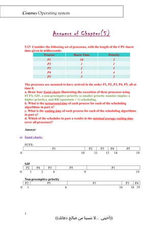
1. Course: Operating system
Answers of Chapter(5)
5.13 Consider the following set of processes, with the length of the CPU-burst
time given in milliseconds:
PriorityBurst TimeProcess
310P1
11P2
32P3
41P4
25P5
The processes are assumed to have arrived in the order P1, P2, P3, P4, P5, all at
time 0.
a. Draw four Gantt charts illustrating the execution of these processes using
FCFS, SJF, a non-preemptive priority (a smaller priority number implies a
higher priority), and RR (quantum = 1) scheduling.
b. What is the turnaround time of each process for each of the scheduling
algorithms in part a?
c. What is the waiting time of each process for each of the scheduling algorithms
in part a?
d. Which of the schedules in part a results in the minimal average waiting time
(over all processes)?
Answer:
a) Gantt charts:
FCFS:
P1 P2 P3 P4 P5
SJF
P2 P4 P3 P5 P1
Non-preemptive priority
P2 P5 P1 P3 P4
..... ))‫ل‬ ‫أخيتي‬‫تنسينا‬‫من‬‫صالح‬((‫دعائك‬
1
0 10 11 13 14 19
0 1 2 4 9 19
0 1 6 16 18 19

2. Course: Operating system
RR (quantum = 1)
P1 P2 P3 P4 P5 P1 P3 P5 P1 P5 P1 P5 P1 P5 P1
b) Turnaround time = finish time- arrival time
OR: Turnaround time = CPU burst time+ wait time
By using the first law (Turnaround time = finish time- arrival time) and getting finish time
from Gantt chart:
Turnaround time
FCFS RR SJF Priority
P1 10-0=10 19-0=19 19-0=19 16-0=16
P2 11 2 1 1
P3 13 7 4 18
P4 14 4 2 19
P5 19 14 9 6
c) Waiting time = Turnaround time - CPU burst time
Waiting time
FCFS RR SJF Priority
P1 10-10=0 19-10=9 19-10=9 16-10=6
P2 10 1 0 0
P3 11 5 2 16
P4 13 3 1 18
P5 14 9 4 1
Average waiting time 9.6 5.4 3.2 8.2
d) The minimal average waiting time is found in SJF algorithm
* * * *
5.17 Suppose that the following processes arrive for execution at the times
indicated. Each process will run the listed amount of time. In answering the
questions, use non-preemptive scheduling and base all decisions on the
information you have at the time the decision must be made.
Burst TimeArrival TimeProcess
80.0P1
40.4P2
11.0P3
..... ))‫ل‬ ‫أخيتي‬‫تنسينا‬‫من‬‫صالح‬((‫دعائك‬
2
0 1 2 3 4 5 6 7 8 9 10 11 12 13 14 19

3. Course: Operating system
(a) What is the average turnaround time for these processes with the FCFS
scheduling algorithm?
(b) What is the average turnaround time for these processes with the SJF
scheduling algorithm?
(c) The SJF algorithm is supposed to improve performance, but notice that we
chose to run process P1 at time 0 because we did not know that two shorter
processes would arrive soon. Compute what the average turnaround time will be
if the CPU is left idle for the first 1 unit and then SJF scheduling is used.
Remember that processes P1 and P2 are waiting during this idle time, so their
waiting time may increase. This algorithm could be known as future-knowledge
scheduling.
Answer:
a) Average turnaround time with FCFS :
We need to draw the Gantt chart to find the finish time then calculate the turnaround time
(Turnaround time = finish time- arrival time)
P1 P2 P3
turnaround time
P1 8-0=8
P2 12-0.4=11.6
P3 13-1=12
Average turnaround
time
10.53
b)Average turnaround time with SJF :
We need to draw the Gantt chart to find the finish time then calculate the turnaround time
(Turnaround time = finish time- arrival time)
P1 P3 P2
turnaround time
P1 8-0=8
P2 13-0.4=12.6
P3 9-1=8
Average turnaround
time
9.53
..... ))‫ل‬ ‫أخيتي‬‫تنسينا‬‫من‬‫صالح‬((‫دعائك‬
3
0 8 12 13
0 8 9 13

4. Course: Operating system
c) Average turnaround time with future-knowledge scheduling.
We need to draw the Gantt chart to find the finish time then calculate the turnaround time
(Turnaround time = finish time- arrival time)
P3 P2 P1
turnaround time
P1 14-0=14
P2 6-0.4=5.6
P3 2-1=1
Average turnaround
time
6.87
* * * *
5.9 Which of the following scheduling algorithms could result in starvation?
a. First-come, first-served
b. Shortest job first
c. Round robin
d. Priority
Answer:
In FCFS algorithm, all jobs is executed in sequence & no job will wait for infinity to be executed
 So, No starvation
SJF could make some long jobs wait for infinity to be executed if shorter jobs continuously arrive
to the ready queue  So, SJF could result in starvation.
RR treats all jobs equally and no job will wait for infinity to be executed  So, No starvation
Priority algorithm could make some low-priority jobs wait for infinity to be executed if higher-
priority jobs continuously arrive to the ready queue  So, Priority algorithm could result in
starvation.
Finally, Shortest job first (SJF) and priority-based scheduling algorithms could result in
starvation.
* * * *
5.7 Explain the differences in the degree to which the following scheduling
algorithms discriminate in favor of short processes:
a. FCFS
b. RR
c. Multilevel feedback queues
Answer:
a. FCFS—discriminates against short jobs since any short jobs arriving after long jobs will have a
longer waiting time.
b. RR—treats all jobs equally (giving them equal bursts of CPU time) so short jobs will be able to
leave the system faster since they will finish first.
..... ))‫ل‬ ‫أخيتي‬‫تنسينا‬‫من‬‫صالح‬((‫دعائك‬
4
0 1 2 6 14

5. Course: Operating system
c. Multilevel feedback queues work similar to the RR algorithm— they discriminate favorably
toward short jobs.
* * * *
5.8 Consider the exponential average formula used to predict the length of the
next CPU burst. What are the implications of assigning the following values to
the parameters used by the algorithm?
a. α= 0 and τ0 = 100milliseconds
b. α= 0.99 and τ0 = 10milliseconds
Answer:
a) Τn+1= α * tn + (1- α) * τn
When α = 0 andτ0 = 100 milliseconds, the equation will be:
Τn+1= 0* tn + (1- 0) * 100 = 100 milliseconds
So, in this case the formula always makes a prediction of (100 milliseconds) for
the next CPU burst.
b) Τn+1= α * tn + (1- α) * τn
. When α = 0.99 and τ0 = 10 milliseconds, the equation will be:
Τn+1= 0.99* tn + (1- 0.99) * 10 = [ 0.99 tn + 0.1] milliseconds
So, in this case the most recent behavior (tn ) of the process is given much higher
weight (99% with comparison to 1%) than the past history associated with the
process (τn=10).
* * * *
5.4 What advantage is there in having different time-quantum sizes at different
levels of a multilevel queuing system?
Answer:
Processes that need more frequent servicing, for example, interactive processes such
as editors, can be in a queue with a small time quantum (because it has high
input/output interrupts).
Processes with no need for frequent servicing (e.g. batch process) can be in a queue
with a larger quantum, requiring fewer context switches to complete the processing
(because it has very low input/output interrupts).
So, the multilevel queuing algorithm makes more efficient use of the computer.
* * * *
Good Luck
..... ))‫ل‬ ‫أخيتي‬‫تنسينا‬‫من‬‫صالح‬((‫دعائك‬
5

6. Course: Operating system
Reem Al_Salih
..... ))‫ل‬ ‫أخيتي‬‫تنسينا‬‫من‬‫صالح‬((‫دعائك‬
6

7. Course: Operating system
Reem Al_Salih
..... ))‫ل‬ ‫أخيتي‬‫تنسينا‬‫من‬‫صالح‬((‫دعائك‬
6