TCSPC (Time-Correlated Single-Photon Counting) complete information

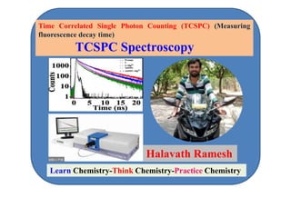
1. Time Correlated Single Photon Counting (TCSPC) (Measuring
fluorescence decay time)
TCSPC Spectroscopy
Halavath Ramesh
Learn Chemistry-Think Chemistry-Practice Chemistry

3. Time-resolved fluorescence lifetime measurements
The radiative emission of light from a molecule after excitation has a multiparameter nature. The
objective of a measurement is therefore to gain information concerning as many parameters as
possible.
 A steady state measurement of the fluorescence emission (intensity vs wavelength) gives an
average and also relative representation.
 The fluorescence lifetime gives an absolute ( independent of concentration) measure and allows a
dynamic picture of the fluorescence to be obtained.
 The fluorescence decay:
 The decay of the excited state of a molecules to the ground state can be expressed as
I(t)= I0 exp(-t/τ)

4. Where ,Io is the intensity at time zero (upon excitation) and τ is the life time . In term of rate
constant (kr—radiative rate, knr– non radiative rate) the life time can be written as below, which
can be compared to the fluorescence quantum yield(Ø).
τ = 1/kr+Knr
Ø = kr/kr + knr
The fluorescence(FL) signal is multiparametric and can be considered as follows, along with the
measurement that can elucidate them,
FL= f(I, λexc,λem, p,ϰ, t)

5. Where ;
I = intensity-measurement is quantum yield (Ø)
λ exc = excitation wavelength- measurement of absorption spectrum
λem= emission wavelength - measurement of fluorescence spectrum
P = polarisation-measurement of anisotropy
X= position- measurement of fluorescence microscopy
t= time- measurement of fluorescence lifetime.
 Although the decay law is based on first order kinetics, in practice, many
fluorescence decays are more complex. Often population of excited molecules are in an
in homogeneous environment, and quenching processes and other environment
influences can lead to multi or non-exponential decay behaviour.

6. TCSPC(Time-Correlated Single –Photon Counting)
 Time –Correlated single-photon counting is the most popular method of determining
picosecond to microsecond fluorescence lifetime.
 It is based on the fact that the probability of detection of a single photon at a certain
time after an excitation pulse is proportional to the fluorescence intensity at that time.
 It is pulsed technique that build up a histogram of fluorescence photon arrival times
from successive excitation-collection cycles.
Instrumentation:
 In generally the instrumentation can be divided into four parts
1. Light sources 2. Detector 3. Electronic 4. Optical components
(instrumental response)2= (optical excitation pulse)2 + (detector transit time
spread)2+ (electronic jitter)2+(optical dispersion)2

7. Fluorescence related techniques have been used intensively in recent years especially in
biology, medicine and biomedical fields for example in imaging, sensing and microscopy.
Observation of the fluorescence emission can provide quantitative information about the
the local environment of the fluorophore, such as the pH, polarity, ion concentration,
molecular interaction and viscosity. bullet This information can be obtained through
several fluorescence features such as lifetime, position, intensity, the excitation and
emission wavelength and polarization. Using the Single Photon Counting (SPC) technique
for imaging has the advantages of high sensitivity, large dynamic range and very good
signal-to-noise ratio. For that reason, this technique is suitable for very low light excitation
condition and low dye concentration allowing to reduce the photo-toxicity and bleaching.
Wide-field imaging allows parallel acquisition of positional information. In order to obtain
lifetime information using SPC, the sample has to be excited with a pulsed source and the
arrival time of every photon generated by the excitation to be measured. The commonly
used techniques for Time-Correlated Single Photon Counting (TCSPC) include one-
dimensional detectors (e.g. photomultiplier tubes or Single Photon Avalanche
Photodiodes) and require the scanning of the sample. This, in addition to the electronics
inherent dead time, decreases the system efficiency and the maximum frame rate. Using a
two-dimensional detector can partially address the problem but such detectors are usually
not sensitive enough to acquire single photon events nor to achieve fast timing (e.g. CCD-
detectors) or reduce the detection ability to one photon at a time (microchannel plate
with quadrant anode).

8. Although the phenomenon of molecular fluorescence emission contains both
spectral (typically UV/visible) and time (typically 10–9 s) information, it is the former
which has traditionally been more usually associated with routine analytical
applications of fluorescence spectroscopy. A photon is a ‘quantized field’, it always
travels at the speed of light and has a momentum, but no mass, and no charge . It does
not decay . TCSPC was soon widely used for time-resolved spectroscopy, and in
particular the measurement of fluorescence lifetimes in solutions. Flash lamps used
kHz repetition rates , but lasers, with pico second excitation pulses at MHz repetition
rates, sped up the measurements significantly and advanced this field enormously. In
conventional TCSPC spectroscopy, single point detectors are typically used to collect a
fluorescence decay curve. In TCSPC, if the sample emits an average of z¯ photons per
excitation cycle, according to the Poissonian distribution the probability pn ph that
exactly n photons are emitted after one excitation pulse.

9. How many of these photons are detected depends on the detector quantum
efficiency q. In addition, TCSPC detector and electronics have a dead-time
(time needed for the detector and the electronics to recover) and, for TAC-
based TCSPC implementation, can typically only detect a maximum of one
photon per excitation pulse. In practice this means that the count rate cannot
exceed the inverse dead time, and a useful count rate of half the inverse dead
time has been defined . The effect of such a dead time is typically not the
distortion of fluorescence decay curves, but a loss of photons.

10. Time-correlated single photon counting (TCSPC) is a remarkable technique for
recording low-level light signals with extremely high precision and picosecond-time
resolution. TCSPC has developed from an intrinsically time-consuming and one-
dimensional technique into a fast, multi-dimensional technique to record light signals. So
this reference and text describes how advanced TCSPC techniques work and
demonstrates their application to time-resolved laser scanning microscopy, single
molecule spectroscopy, photon correlation experiments, and diffuse optical tomography
of biological tissue. It gives practical hints about constructing suitable optical systems,
choosing and using detectors, detector safety, preamplifiers, and using the control
features and optimising the operating conditions of TCSPC devices.
Advanced TCSPC Techniques is an indispensable tool for everyone in research and
development who is confronted with the task of recording low-intensity light signals in
the picosecond and nanosecond range.

11. Time-correlated single-photon counting (TCSPC) is a well established and a common
technique for fluorescence lifetime measurements, it is also becoming increasingly
important for photon migration measurements, optical time domain reflectometry
measurements and time of flight measurements.
The principle of TCSPC is the detection of single photons and the measurement of
their arrival times in respect to a reference signal, usually the light source. TCSPC is a
statistical method requiring a high repetitive light source to accumulate a sufficient
number of photon events for a required statistical data precision.
TCSPC electronics can be compared to a fast stopwatch with two inputs. The clock is
started by the START signal pulse and stopped by the STOP signal pulse. The time
measured for one START – STOP sequence will be represented by an increase of a
memory value in a histogram, in which the channels on the x-axis represent time.
With a high repetition rate light source millions of START – STOP sequences can be
measured in a short time. The resulting histogram counts versus channels will
represent the fluorescence intensity versus time.

67. DAS6
Fluorescence decay analysis software
 DAS6 is HORIBA’s software for analysis of time domain fluorescence life time.
 Data files measured using “ Data station” on HORIBA Scientific instruments can be
opened directly and facilities are provided to import data from other instruments and
software packages.
 DAS6 provides multi-exponential fitting plus a number of modules for analysis of
more specialized fluorescence decay processes. There is an optical module allowing for
a non-extensive decay distribution fit.
The key feature of DAS6 are:
Decay modules include:
1. Exciplex kinetics
2. Distribution
3. Exponential series
4. Foster energy transfer

68. 5. Yokota-Tanimoto energy transfer
6. Micellar quenching
7. Anisotropy analysis
8. Batch exponential analysis
9. Global exponential analysis
Optical decay modules include:
* Non-extensive distribution