This document discusses the relationship between electricity and magnetism through the lens of relativity. It begins by explaining how early discoveries in magnetism led to modern insights unifying electric and magnetic forces through relativity. It then provides Einstein's perspective on how the electromotive force acting on a moving body in a magnetic field is really an electric field. The document goes on to derive the magnetic Lorentz force experienced by a moving charge near a current-carrying wire using relativistic transformations and Lorentz contraction. It concludes by analyzing the complex equations of motion governing particles in a Wien mass filter, which uses electric and magnetic fields to select specific ions.

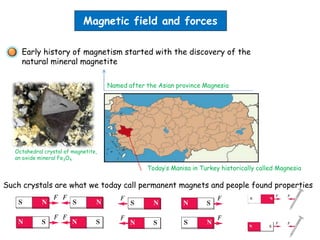
1. Magnetic field and forces
Early history of magnetism started with the discovery of the
natural mineral magnetite
Named after the Asian province Magnesia
Octahedral crystal of magnetite,
an oxide mineral Fe3O4
Today’s Manisa in Turkey historically called Magnesia
Such crystals are what we today call permanent magnets and people found properties

2. Chinese compass
invented 2230 years ago
Modern HDD
Instead of following the traditional (textbook) approach to first introduce the
phenomena we start by highlighting here the modern insight that
Electric forces and fields and magnetic forces and
fields are unified through relativity
What led me more or less directly to the special theory of relativity was the conviction
that the electromotive force acting on a body in motion in a magnetic field was nothing
else but an electric field.
-Einstein 1953-
http://en.wikipedia.org/wiki/Relativistic_electromagnetism

3. The origin of magnetic forces on a moving electric charge
A first hint at a fundamental connection between electricity and magnetism
comes from Oersted’s experiment
Electric phenomenon Magnetic phenomenon
A distribution of electric charges
creates an E-field
A moving charge or a current creates (an
additional) magnetic field
The E-field exerts a force F=q E on any
other charge q
The magnetic field exerts a force F on
any other moving charge or current

4. Where are the moving charges or currents in a permanent magnet?
We see later more clearly that these are the “moving electrons” on an
atomic level (angular momentum L, spin S, J=L+S)
How can relativity show that a moving charge next to a current
experiences a force
wire of
infinite length
Negative charge (electrons) flowing to the right
Stationary positive ions
drift velocity of
electrons, remember
Drude model of
conductivity
Let’s consider the special case that our test charge outside the wire moves likewise with
v, the drift velocity of the electrons in the wire
Now we look at the situation from the perspective of the moving test charge q:
charge density
0
/
Q l
 
we transform into the moving coordinate system of the test charge

5. From the perspective (moving reference frame) of the test charge electrons are at rest
and ions move
Now the “magic” of special relativity kicks in:
http://www.physicsclassroom.com/mmedia/specrel/lc.cfm
Spaceship moving with
10% of speed of light
Spaceship moving with
86.5% of speed of light
Lorentz-contraction quantified by
2
0 1
v
l l
c
 
   
 

6. Due to Lorentz-contraction:
test charge sees modified charge density for moving + ions
Q
l
  2
0 1
Q
v
l
c

 
  
 
2
1
v
c


 
  
 
test charge sees imbalance of charge
density for electrons and + ions
Since v-drift is about 0.1 mm/s <<c (see http://physics.unl.edu/~cbinek/Unit_13%20Current%20resistance%20and%20EMF.pptx) we
can expand into Taylor series around x=v/c=0
2
2
2
1 1
( ) (0) (0) (0) ... 1 ...
2 2
1
x
f x f f x f x
x
 
       

2
2
2
v
c

 
  
Charge density of ions increased in the frame of the test charge

7. Likewise in comparison to lab frame (frame of the wire) the electrons are
now seen at rest (were moving in the lab frame)
2
2
2
v
c

test charge sees charge density of electrons reduced by
(because test charge at rest sees wire as neutral despite moving negative charges)
Net effect: wire neutral in the lab frame gets charge density
2
2
v
c

in the frame of moving electron
Remember the electric field of an infinite wire with homogeneous
charge density 
Gaussian cylinder of radius r
2
0
2
Q
E d r E r l


 

l
0
2
E
r




8. For the moving charge in the moving frame we have
2
2
v
c

 
Moving charge sees an electric field
2
2
0
1
2
v
E
r c



charge is exerted to a force away from the wire
2
2
0
2
q v
F
r c



In the lab frame (frame of the wire) we interpret this as the magnetic Lorentz force
2
0
2
v
F qv qvB
r c


  with 0 0
2
0
2 2 2
v v I
B
r c r r
 
 
  
  
magnetic B-field in distance r from a wire carrying the current I
2
0 0
1
c
 


9. Our expression F qvB
 holds for the special case v B

I
v
B
F qvB

In general: F q v B
 
magnetic force on a moving charged particle

10. Considering the mathematical cross product structure of the Lorentz
force.
Do you think that this magnetic force can do work on a charge?
Clicker question
1) Yes, it is a force and we can evaluate Fdr

2) No, the integral will always be zero
Fdr

3) Yes, the integral will equal qvBl where l is the length of the path
Fdr


11. B known from current through
Helmholtz coils
The e/m tube demonstration
We see Lorentz force F  v and hence  dr no work
Circular orbit
2
v
qvB m
R

v known from Ekin=qVab
measure R vs. B
e/m= 1.76 x 1011 C/kg
With v R


:
c
qB
m
 
 
Cyclotron frequency
http://en.wikipedia.org/wiki/Cyclotron
𝑞
𝑚
=
𝑣
𝐵𝑅

12. F qv B qvB
 
 
From we can determine the unit of the B-field
[ ]
[ ] :
[ ][ ] /
F N N
B T
q v As m s Am
   
1T=1tesla=1N/Am in honor of Nikola Tesla http://en.wikipedia.org/wiki/Nikola_Tesla
A moving charged particle in the presence of an E-field and B-field
 
F q E v B
  
An application in modern research: the Wien mass filter
http://www.specs.de/cms/front_content.php?idart=148
Resolution:
m/Δm > 20@5 keV
It selects defined ions
by a combination of electric
and magnetic fields.

13. aperture aperture
The charged particle will only follow a straight path through the crossed E and
B fields, if net force acting on it is
  0
q E v B
  
For the simple special case:
x
y
z
( ,0,0) , (0, ,0) , (0,0, )
0 0
0 0
x y z
y
v v E E B B
e e e
v B v vBe
B
  
   
  0
y
q E vB e
  E
v
B

Wien filter can be used for mass selection if
incoming particles have fixed kinetic energy
2 /
kin
v E m

zero

14. Is that the whole story of the Wien filter
Absolutely not, as this research manuscript from 1997 indicates

15. Equation of motion for particle of charge q and mass m in the filter:
( , , ) , (0, ,0) , (0,0, )
0 0
x y z
x y z
x y
x y z y x
v v v v E E B B
e e e
v B v v v v Be v Be
B
  
   
 
mr q E v B
  
y
m x qv B

x
m y qE qv B
 
0
m z  ( ) z
z t v t

coupled differential equations, nasty!
But, we are honors students:
Not the goal but the game
Not the victory but the action
In the deed the glory
viewer discretion is advised!
Do not click if you are not prepared
to see nastiness.

16. m x qyB

m y qE qxB
 
qB
x y
m

qB qE qB
x x
m m m
 
 
 
 
We define
introduced earlier already as cyclotron frequency
c
qB
m
 
2 2
x c c x
E
v v
B
 
 
Solving first the homogeneous equation
2
0
x c x
v v

 
Ansatz  
sin
x
v A t
 
 
 
 
cos
sin
x
x
v A t
v A t
  
  
 
  
Substitution into homogeneous differential equation
   
2
2
sin sin 0
c
A t A t
     
     c
 

Solving the inhomogeneous equation
through
2 2
x c x c
E
v v
B
 
 
Solution of inhomogeneous equation is general solution of homogeneous
plus a particular solution of inhomogeneous
For the particular solution we try x
v const

Back to x
x v


17. 0
x
v 
2 2
x c x c
E
v v
B
 
 
With x
E
v
B
 is a solution
General solution of inhomogeneous differential equation
   
sin cos
x c c
E
v a t b t
B
 
  
   
( ) cos sin
c c
c c
E a b
x t t t t c
B
 
 
   
With x(t=0)=0 / c
c a 

 
   
( ) 1 cos sin
c c
c c
E a b
x t t t t
B
 
 
   
c c
E
y x
B
 
 
 
   
( )
1 cos sin
c c
c c
E
y t x t c
B
a t b t c
 
 
  
    
particular solution of
inhomogeneous differential eq.
general solution of
homogeneous differential eq.

18.    
sin cos
c c
c c
a b
y at t t ct d
 
 
     
Final adjustment of initial conditions:
0
( 0)
x x
E
v t v b
B
    0
x
E
b v
B
 
0
( 0)
y y
v t v c
  
0
( 0)
c
b
y t y d

   
0
(0)
x c y c
v v a
 
  0
y
a v c
 
 
   
0 0
( ) 1 cos sin
y x
c c
c c c
v
E v E
x t t t t
B B
 
  
 
    
 
 
   
 
0 0
0
( ) sin 1 cos
y x
c c
c c c
v v E
y t y t t
B
 
  
 
    
 
 
m x qyB


19. Can we recover the simple case of acceleration free motion?
Motion is simple for 0
( 0) 0
y y
v t v
   and 0
( 0) 0
y t y
  
from
   
 
0 0
0
( ) sin 1 cos
y x
c c
c c c
v v E
y t y t t
B
 
  
 
    
 
 
motion with y(t)=0 for the entire path in the filter
=0
This is of course the condition
0
x
E
v
B

aperture aperture
x
y
z
No net force
In fact:
 
   
0 0
( ) 1 cos sin
y x
c c
c c c
v
E v E
x t t t t
B B
 
  
 
    
 
 
( )
E
x t t
B

=0
=0
=0 =0

20. In general motion is very complex
Let’s consider charged particle with mass
M0 moving with constant v through EXB
particle with mass M=M0 / has different
initial v than particle with M0
Trajectory deviates from straight line
If  significantly deviates from 1
trajectory can be very complicated and may spoil
mass filter effect,
see trajectory for =4

21. Other E x B devices
Common concept of plasma based cross-field devices:
A magnetic field traps electrons in a plasma giving rise to reduced electron
conductivity and thus allowing for maintaining a large electric field in the
plasma
Examples:
Hall-effect thruster: Ion thruster used in spacecraft propulsion
https://commons.wikimedia.org/wiki/File:HallThruster_2.jpg
Xenon ions are accelerated towards
cathode in the region of
reduced conductivity

22. Example from material science:
Magnetron discharge: employed in magnetron sputtering for thin film deposition
Electrons generated at the cathode are trapped along the
field lines until they undergo collision
Residence time of electrons in cathode region considerably
increased
Operation of discharge at low pressure possible because
electron can ionize gas even though electron free path
larger than cathode-anode gap
http://ncmn.unl.edu/thinfilm/aja-sputtering-system

23. Physics of collisional electron transport in E x B
In a plasma, electrons can’t travel freely but collide with other
particles at a rate 𝑓 =
1
𝜏
In steady state, momentum change from field forces and
momentum change from collision cancel
𝐹 𝜏 +
Δ𝑃
𝜏
𝜏 = 0
𝐹 +
Δ𝑃
𝜏
= 0
𝑞 𝐸 + 𝑣 × 𝐵 −
m𝑣
𝜏
= 0
𝑒0
𝑚
𝐸 + 𝑣 × 𝐵 + 𝑓𝑣 = 0
With 𝐸 = 𝐸𝑒𝑥 and 𝐵 = 𝐵𝑒𝑦 𝑣 × 𝐵 =
𝑒𝑥 𝑒𝑦 𝑒𝑧
𝑣𝑥 𝑣𝑦 𝑣𝑧
0 𝐵 0
= −𝑣𝑧𝐵𝑒𝑥 + 𝑣𝑥𝐵𝑒𝑧
𝑒0
𝑚
𝐸 − 𝑣𝑧𝐵 = −f vx
𝑒0
𝑚
𝑣𝑥𝐵 = −f vz 𝑣𝑥 = −f
vz
𝜔𝑐𝑒
𝑒0
𝑚
𝐸 − 𝜔𝑐𝑒𝑣𝑧 =
𝑓2
𝑣𝑧
𝜔𝑐𝑒
𝑣𝑧 =
𝑒0
𝑚
𝐸
1
𝜔𝑐𝑒 +
𝑓2
𝜔𝑐𝑒
𝑣𝑥 = −
𝑒0
𝑚
𝐸
𝑓
𝜔𝑐𝑒
2
+ 𝑓2

24. For 𝜔𝑐𝑒≫f which means electron makes many orbits before it collides
with another particle (given for the case of a Hall thruster)
𝑣𝑧 =
𝑒0
𝑚
𝐸
1
𝜔𝑐𝑒 +
𝑓2
𝜔𝑐𝑒
𝑣𝑥 = −
𝑒0
𝑚
𝐸
𝑓
𝜔𝑐𝑒
2
+ 𝑓2
𝑣𝑥 ≈ −
𝑒0
𝑚
𝐸
𝑓
𝜔𝑐𝑒
2 = −
𝑒0
𝑚
𝐸
𝑓𝑚
𝜔𝑐𝑒𝑒0𝐵
= −
𝐸
𝐵
𝑓
𝜔𝑐𝑒
𝑣𝑧 ≈
𝑒0
𝑚
𝐸
𝜔𝑐𝑒
=
𝐸
𝐵
From this we see that the mobility of the electrons parallel to the electric field
𝜇𝑒,𝐸 =
𝑣𝑥
𝐸
=
𝑓
𝐵𝜔𝑐𝑒
is strongly reduced when compared to the case B=0
𝑒0
𝑚
𝐸 − 𝑣𝑧𝐵 = −f vx
where yields
𝑒0
𝑚
𝐸 = −f vx
and thus
𝜇𝑒,𝐸(𝐵 = 0) =
𝑣𝑥
𝐸
=
𝑒0
𝑚 𝑓
In the absence of collisions electrons would be perfectly trapped