1. RSSI based localization in wireless sensor networks:
Introduction :
Wireless sensor networks(WSN) are large-scale embedded systems with many nodes and use standardized platforms to transport data
either for analysis at a server or for computing directly in the network. The nodes in the network are physically distributed and may fail or
be introduced to the network over time. Location information can have many uses in sensor networks and here we describe a localization
algorithm and its implementation.
The strength of received power from a signal can be used to estimate distance because all electromagnetic waves have inverse-square
relationship between received power and distance .Usually received signal strength indicator (RSSI) is used to represent the
condition of received power level. RSSI is generally implemented in most of the wireless communication standards and can be
converted to a received power by applying offset to calibrate to the correct level..
If the target sensor node can hear more than three sensor nodes which are location aware, trilateration or multilateration can be used to
estimate the location of target node
Trilateration is a method for determining the intersections of three sphere surfaces given the centers and radii of the three spheres.Two
methods of solving the trilateration problem are nonlinear least squares and circle intersections with clustering.
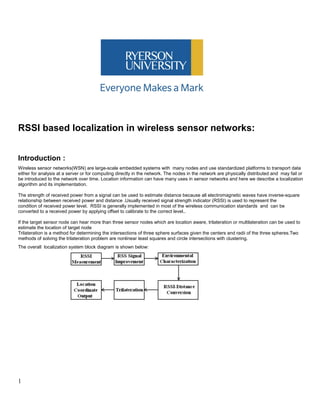
The overall localization system block diagram is shown below:
1

2. Sensor networks physical layer :
WSN rely on battery-operated nodes and wireless data communication. Eliminating wires for power and data allows sensors to be
deployed in environments that are not feasible for traditional sensors. Because batteries have only a limited capacity, that energy must be
conserved. But wireless communication requires more energy than does communication by wire. In addition to traditional energy
conservation techniques, we must develop new networking methods that conserve energy in wireless environments.
In Wireless sensor networks the structure of the connections between nodes is not designed in advance.
Self organize WSN:
Some networks can self organize without intervention of a network administrator which allow users to distribute nodes and let the nodes
organize their communication links for themselves.
In a self organize network :
1) Nodes must be able to declare themselves to be part of the network and to determine what other nodes are in the network.
Admission control policies determine how nodes can be admitted.
2) Network must determine how to route data. Sensor networks generally establish a network structure based on locations of the
nodes. Data then routed based on these communication paths.
3) When nodes enter or leave the network, the network must update its configuration and routing.
Sensor nodes hardware:
Power management and networking are intimately related. The power profiles of sensor nodes help determine the characteristics of
networking protocols. Because communication costs more energy than computation, in-network processing saves energy if it reduces the
volume of data transmitted over the network as a result, nodes can save energy by spending computing cycles to determine when to turn
their radios on and off. Furthermore, sensor node radios spend more energy receiving (Rx) than transmitting(Tx). So nodes spend most of
their time listening so:.
1) Node must be able to turn radio on/off quickly and efficiently. Power wasted during power-up and power-down is not available for
operating the network. Radios in the nodes may need to operate at several different power levels to avoid interference and save
battery power. They may also need to operate at several frequencies to avoid interference.
2) Node must be able to buffer network traffic and make routing decisions.
This approach makes sense for low data rate applications, but higher data rate applications like audio and video benefit from performing
some of the data analysis in network nodes.
In many cases,we can generate abstractions of the raw data that can be transmitted at much less cost. However, processing may require
trading data between nodes, so the net amount of communication must be carefully considered.
2

3. Localization algorithm in WSN requirements :
Due to the high number of sensor nodes only a few of nodes would be given a prior information about their positions with respect to a
global coordinate system(anchor nodes or beacon nodes). The rest of the nodes then calculate their positions and localize themselves by
using positions of the anchors and their own relations with these anchors. There are several challenges for the localization in sensor
networks.:
1. Accuracy. Some applications may require an upper bound on the estimation error.
2. Sparse anchor tolerance. Even with very few anchors the system should be able to function and localize the nodes without initial
position information.
3. Error tolerance. The localization algorithm must work with range measurement errors. Range errors occur because of the ¯nite
Signal to Noise Ratio SNR of the received signals to perform ranging or any kind of relationship. Also sampling effects can induce
measurement errors.
4. Scalability. A scalable algorithm keeps the required per-node computation constant as the network size grows. This property is
critical to be able to support networks of different sizes without redesigning the localization system.
5. Energy dissipation. It is desirable to minimize total computation energy in the network. However, there is often a tradeff between
computation energy,speed of convergence, and communication requirements. in addition it is also desirable to keep the total
energy spent on communication as low as possible.
6. Convergence time. Applications may need fast convergence times, for ex-ample becomes critical if a mobile node, which can be
attached to a human,localizes itself.
7. Solution has to be tolerant to large errors in range measurements.
8. Solution has to be tolerant to large errors in range measurements.
9. Complexity of the localization algorithm must not grow faster than the network size.
10. Algorithm should consume low power and requiring minimal communication.
11. Wireless sensor network nodes have limited processing power individually so indoor location estimation algorithms must be
simple for implementation.
First group that will be reviewed include centralized algorithms followed by a study of distributed approaches.
Localization algorithms can be divided in two types:
Centralized localization computations :
data is collected to a single unit and the location of all the nodes are computed all at once within this unit. The most common issue raising
from centralized computations is:
1) Communication overhead for bringing the data to the computation node.
2) Distributing the computed positions from the computation node to the rest of the nodes in the network also adds communication
overhead.
3) In centralized algorithms computation complexity for the processing node grow with a more than linear relationship. That is
increasing the network size increases the load on the processing node more than the load increase in a distributed computation
node.
Distributed localization algorithms :
Due to the inherent distributed structure of sensor networks a distributed solutions is more appropriate for sensor network localization. One
general problem with the distributed algorithms approach is that convergence of the results can take long which maybe inappropriate for
some applications.
3

4. However when there are range errors the solution does have an error. In the case with noisy range measurements, having more reference
points than necessary can create an averaging effect as the range error in each measurement would have varying errors. Such a solution
could be implemented using optimization techniques such as Least Squares optimization. Accuracy of the ranging measurements is a
challenge .
RRSI based localization System Block Diagram Design
Signal processing and data mining blocks are the core of information handling system.
First task in location system design work is defining how the system converts raw RSSI signal to location coordinate (valuable
information). It has to go through several processing steps as shown below.
RSSI values are collected from reference nodes in distance estimation step. Using these RSSI values, we can perform environmental
characterization to find suitable parameters for that area.
When calibration process is over, the environmental parameters are fixed and will not be change unless large changes happen to the
objects within the area.
I
The next step is to obtain continuous RSSI values from the reference nodes in the online operation.
From RSSI-Distance conversion distances between target sensor node and the reference nodes can be obtained.
With both RSSI values and environmental parameters ready, we can convert those RSSI values into distance using path loss model:
4

5. where P(d0) is the received power measured at distance d0. Generally, d0 is fixed as a constant d0 = 1 m. Path loss exponent n is
parameters for environmental characterization.
After the step of environmental characterization, the two main environmental parameters n and Pr(d0) are obtained. Thus, the distance
between transmitter and receiver can be estimated using the following expression
Wireless sensor network nodes have limited processing processing power individually so indoor location estimation algorithms must be
simple for implementation.
For ensuring faster processing and tool-independent programming algorithms, mathematical calculations and processing must be simple
and programmable to any low-power cpu with limitation and constraints. The main computational loads are:
Computation of RSSI-distance conversion is not easy to be implemented in a resource and computational power limited sensor node. This
is because the computation of exponential function , which generates large number if the input data is not stable. Taylor series can be used
to avoid exponential computation and simplify the calculation by selecting appropriate length of expression L below :
RSSI Trilateration algorithm design:
Trilateration is a distributed localization algorithm and its functionality does not depend on the anchor density.
For ensuring faster processing and tool-independent programming algorithms, mathematical calculations and processing must be simple
and programmable to any low-power cpu with limitation and constraints. The main computational loads are:
Computation of RSSI-distance conversion is not easy to be implemented in a resource and computational power limited sensor node. This
is because the computation of exponential function , which generates large number if the input data is not stable.
Taylor series can be used to avoid exponential computation and simplify the calculation by selecting appropriate length of expression L
below :
#include <iostream>
#include <cmath>
#include <iomanip>
using namespace std;
long double log_tylor(long double y ,int precision )
{
long double totalValue = 0; //The summation of each polynomial evaluated
5

6. bool reciprocal = false; //Flag to use if greater than 2
long double count = 1; //Keeps track of the count in the loop
if (y > 2.0) //Use the rule -ln(1/x) == ln(x) to keep accuracy
{
y = 1 / y; //Change to using 1/x rather than x
reciprocal = true; //Flag as true (sign change is later)
}
while (count < precision)
{
totalValue += pow(-1, count + 1) * (pow((y-1),count)/count);
count++;
}
if (reciprocal == true)
totalValue *= -1; //If reciprocal was used multiply by -1 to change sign
//cout << "Distance is:" << setprecision(5) << totalValue << endl;
return totalValue;
}
int RSSI_Conversion()//main()
{
int precision; // The the highest order of polynomial to use.
long double x; // Value to evaluate to ln for.
/***************Get User Input***************/
cout << "Precision=";
cin >> precision;
cout << "RSSI_1=";
cin >> x;
/***************End User Input***************/
//Get actual value using log(x) found in <cmath>
cout << "The log(x) C++ function value is:" << log(x) << endl;
cout << "Distance is:" << setprecision(5) << log_tylor(x ,precision ) << endl;
return 1;
}
Trilateration estimation can find an unknown location from several reference locations. In trilateration, the distances between reference
locations and the unknown location can be considered as the radii of many circles with centers at every reference location. Thus, the
unknown location is the intersection of all the sphere surfaces. as shown here:
6

7. In general coordinates, three spheres intersect
To simplify the problem, define basis vectors
In this new coordinate system, you can write the three points as
System of three equations can now be written as:
the above system of three equations is easy to solve:
7

8. In the original coordinates, the solution is:
Trilateration Implementation:
#include <stdio.h>
#include <math.h>
/* Largest nonnegative number still considered zero */
#define MAXZERO 0.0
typedef struct vec3d vec3d;
struct vec3d {
double x;
double y;
double z;
};
/* Return the difference of two vectors, (vector1 - vector2). */
vec3d vdiff(const vec3d vector1, const vec3d vector2)
{
vec3d v;
v.x = vector1.x - vector2.x;
v.y = vector1.y - vector2.y;
v.z = vector1.z - vector2.z;
return v;
}
/* Return the sum of two vectors. */
vec3d vsum(const vec3d vector1, const vec3d vector2)
{
vec3d v;
v.x = vector1.x + vector2.x;
v.y = vector1.y + vector2.y;
v.z = vector1.z + vector2.z;
return v;
}
/* Multiply vector by a number. */
vec3d vmul(const vec3d vector, const double n)
8

9. {
vec3d v;
v.x = vector.x * n;
v.y = vector.y * n;
v.z = vector.z * n;
return v;
}
/* Divide vector by a number. */
vec3d vdiv(const vec3d vector, const double n)
{
vec3d v;
v.x = vector.x / n;
v.y = vector.y / n;
v.z = vector.z / n;
return v;
}
/* Return the Euclidean norm. */
double vnorm(const vec3d vector)
{
return sqrt(vector.x * vector.x + vector.y * vector.y + vector.z * vector.z);
}
/* Return the dot product of two vectors. */
double dot(const vec3d vector1, const vec3d vector2)
{
return vector1.x * vector2.x + vector1.y * vector2.y + vector1.z * vector2.z;
}
/* Replace vector with its cross product with another vector. */
vec3d cross(const vec3d vector1, const vec3d vector2)
{
vec3d v;
v.x = vector1.y * vector2.z - vector1.z * vector2.y;
v.y = vector1.z * vector2.x - vector1.x * vector2.z;
v.z = vector1.x * vector2.y - vector1.y * vector2.x;
return v;
}
/* Return zero if successful, negative error otherwise.
* The last parameter is the largest nonnegative number considered zero;
* it is somewhat analoguous to machine epsilon (but inclusive).
*/
int trilateration(vec3d *const result1, vec3d *const result2,
const vec3d p1, const double r1,
const vec3d p2, const double r2,
const vec3d p3, const double r3,
const double maxzero)
{
vec3d ex, ey, ez, t1, t2;
double h, i, j, x, y, z, t;
/* h = |p2 - p1|, ex = (p2 - p1) / |p2 - p1| */
ex = vdiff(p2, p1);
h = vnorm(ex);
if (h <= maxzero) {
/* p1 and p2 are concentric. */
9

10. return -1;
}
ex = vdiv(ex, h);
/* t1 = p3 - p1, t2 = ex (ex . (p3 - p1)) */
t1 = vdiff(p3, p1);
i = dot(ex, t1);
t2 = vmul(ex, i);
/* ey = (t1 - t2), t = |t1 - t2| */
ey = vdiff(t1, t2);
t = vnorm(ey);
if (t > maxzero) {
/* ey = (t1 - t2) / |t1 - t2| */
ey = vdiv(ey, t);
/* j = ey . (p3 - p1) */
j = dot(ey, t1);
} else
j = 0.0;
/* Note: t <= maxzero implies j = 0.0. */
if (fabs(j) <= maxzero) {
/* p1, p2 and p3 are colinear. */
/* Is point p1 + (r1 along the axis) the intersection? */
t2 = vsum(p1, vmul(ex, r1));
if (fabs(vnorm(vdiff(p2, t2)) - r2) <= maxzero &&
fabs(vnorm(vdiff(p3, t2)) - r3) <= maxzero) {
/* Yes, t2 is the only intersection point. */
if (result1)
*result1 = t2;
if (result2)
*result2 = t2;
return 0;
}
/* Is point p1 - (r1 along the axis) the intersection? */
t2 = vsum(p1, vmul(ex, -r1));
if (fabs(vnorm(vdiff(p2, t2)) - r2) <= maxzero &&
fabs(vnorm(vdiff(p3, t2)) - r3) <= maxzero) {
/* Yes, t2 is the only intersection point. */
if (result1)
*result1 = t2;
if (result2)
*result2 = t2;
return 0;
}
return -2;
}
/* ez = ex x ey */
ez = cross(ex, ey);
x = (r1*r1 - r2*r2) / (2*h) + h / 2;
y = (r1*r1 - r3*r3 + i*i) / (2*j) + j / 2 - x * i / j;
z = r1*r1 - x*x - y*y;
10

11. if (z < -maxzero) {
/* The solution is invalid. */
return -3;
} else
if (z > 0.0)
z = sqrt(z);
else
z = 0.0;
/* t2 = p1 + x ex + y ey */
t2 = vsum(p1, vmul(ex, x));
t2 = vsum(t2, vmul(ey, y));
/* result1 = p1 + x ex + y ey + z ez */
if (result1)
*result1 = vsum(t2, vmul(ez, z));
/* result1 = p1 + x ex + y ey - z ez */
if (result2)
*result2 = vsum(t2, vmul(ez, -z));
return 0;
}
int main(void)
{
vec3d p1, p2, p3, o1, o2;
double r1, r2, r3;
int result;
while (fscanf(stdin, "%lg %lg %lg %lg %lg %lg %lg %lg %lg %lg %lg %lg",
&p1.x, &p1.y, &p1.z, &r1,
&p2.x, &p2.y, &p2.z, &r2,
&p3.x, &p3.y, &p3.z, &r3) == 12) {
printf("Sphere 1: %g %g %g, radius %gn", p1.x, p1.y, p1.z, r1);
printf("Sphere 2: %g %g %g, radius %gn", p2.x, p2.y, p2.z, r2);
printf("Sphere 3: %g %g %g, radius %gn", p3.x, p3.y, p3.z, r3);
result = trilateration(&o1, &o2, p1, r1, p2, r2, p3, r3, MAXZERO);
if (result)
printf("No solution (%d).n", result);
else {
printf("Solution 1: %g %g %gn", o1.x, o1.y, o1.z);
printf(" Distance to sphere 1 is %g (radius %g)n", vnorm(vdiff(o1, p1)), r1);
printf(" Distance to sphere 2 is %g (radius %g)n", vnorm(vdiff(o1, p2)), r2);
printf(" Distance to sphere 3 is %g (radius %g)n", vnorm(vdiff(o1, p3)), r3);
printf("Solution 2: %g %g %gn", o2.x, o2.y, o2.z);
printf(" Distance to sphere 1 is %g (radius %g)n", vnorm(vdiff(o2, p1)), r1);
printf(" Distance to sphere 2 is %g (radius %g)n", vnorm(vdiff(o2, p2)), r2);
printf(" Distance to sphere 3 is %g (radius %g)n", vnorm(vdiff(o2, p3)), r3);
}
}
return 0;
}
11

12. Trilateration in noisy environment:
The main advantage of Trilateration is that its functionality does not really depend on the anchor density. However when
there are range errors the solution does have an error. In the case with noisy range measurements, having more
reference points than necessary can create an averaging effect as the range error in each measurement would have varying
errors. Such a solution could be implemented using optimization techniques such as Least Squares optimization.
Another important consideration is the accuracy of the ranging measurements. It is obvious that the less noisy the range
measurements are the more accurate the final position estimation would be.
Least-squares Solution:
The method of least squares is a standard approach to the approximate solution of overdetermined systems, i.e., sets of
equations in which there are more equations than unknowns. "Least squares" means that the overall solution minimizes the
sum of the squares of the errors made in the results of every single equation. Least squares corresponds to the maximum
likelihood criterion if the experimental errors have a normal distribution and can also be derived as a method of moments
estimator.
Traingulation using ML
Trilaterationin in large scale sensor network case:
To use Trilateration techniques, at least three reference nodes are required however in larger networks three possible scenarios might
happen:
a) The sensor nodes are able to reach at least three Anchor -node
b) The sensor nodes are able to reach one or two Anchor -nodes only
c) The sensor nodes are not able to reach any Anchor -node
For second and third scenarios collaborative multilaterations and iterative multilaterations were developed to extend solution to for
large scale network.
Atomic multi-lateration is used to estimate the location directly from three or more reference nodes as shown in Fig. 9(a). If all sensor
nodes are able to reach at least three Anchor-nodes, then
atomic multilateration is used.
If sensor nodes are too far away from Anchor-nodes, it is not able to fulfil the requirement of at least three reference nodes. Therefore,
iterative localization may be considered to spread location to other nodes. This approach is called iterative multilateration. In this
approach, sensor nodes are converted to reference nodes after localized by Anchor --nodes as shown in Fig. 9(b). In next step, these
reference nodes can be used to localize other nodes that are not reachable to Anchor --nodes. This process continues until all sensor
nodes in the network are localized.
12

13. In a large scale sensor network, atomic and iterative multi-laterations can be used to localize any sensor nodes if the first scenario happens
at initial state. However, the random allocation of Anchor-nodes could be far to each other. Thus, no sensor node can reach at least three
Anchor -nodes at initial state. This leads to second and third scenarios at initial state.
Localization system Network Implementation
After the flow of location information processing was decided, next step is to implement the operation network. Design goals are: low
power consumption,Low cost , small size, configurable and flexible software, wide radio coverage, good processing ability, sufficient I/O for
sensing and actuating.
Operation network for indoor location system based on WSN is related to the source of raw data and the sink of useful information. Thus,
the characteristics of the WSN implementation for indoor location system are investigated and shown below :
13

14. 1. Network is constructed to support monitoring all the time, thus all sources of information send data constantly to a base station.
2. The network is multi-source single sink data network.
3. The data direction is from source to sink, thus no query service is available.
4. There are two types of network nodes: stationary and mobile nodes
5. All sensor nodes can be an intermediate node for routing packets to base station.
6. Nodes located in the same indoor area can be organized together as a cluster.
7. A cluster consists of both stationary and mobile nodes.
Network Scheduling
Communication signals are initiated from mobile nodes so when mobile node enters a new zone it wakes up all reference nodes. When a
reference node cannot hear any mobile node for more than 10 seconds it automatically switch to inactive mode. To save power reference
nodes are in inactive mode when there is no target node in the area. An accelerometer can be installed into the sensor node to activate
mobile node and the mobile node activates other reference nodes. When a target node moves into the area, the movement of the target
node causes motion sensor to generate activation signal. The activation signal is flooded to activate all reference nodes in the area.
The communication paths are shown here:
1. T2 broadcasts a message to all reference nodes (R1, R3, R5). Reference nodes are awakened and reply to T2 .
2. T2 collects the IDs and RSSI values from all reference nodes and estimate location coordinate of the target node.
3. The location information is then forwarded to base station (B0) .
4. Base station forwards the data to a computer for display and monitoring.
Network performance issue:
Transmission scheduling must be considered in the reference nodes because all reference nodes receive the activation signal from target
node at the same time a few references may send estimation signal for RSS ranging at the same time. Therefore, the target node receives
a few estimation signals to measure RSSI at the same time. Inevitably, packet loss happens leading to operation failure.
There are three kinds of transmission scheduling can be considered in indoor location tracking system implementation:
1. Use a random number generator to produce time delay for the first estimation signal. The duration of delay can be obtained using a
random number (ranged from 0 to 1). Here transmission scheduling may still have signal collision problem as two reference nodes
generate the same random number, the advantage is the ease of implementation.
2. Use a fixed number obtained from the node ID or address to produce time delay for the first estimation signal. We may have problem
when the number of total sensor nodes is large and the transmission period is short. This causes the divided delay time duration too short.
In addition, expansion of network increases the total number of nodes, leading to unnecessary re-installation to all sensor nodes.
3. Use a fixed number obtained from the group ID to produce time delay for the first estimation signal. Group ID is used to differentiate the
sensor nodes within the same indoor area or cluster assigned by cluster head. This is a good choice, but it depends on the good clustering
result of network.
In-network Processing
Due to the size constraint, the individual device in wireless sensor network is normally limited in processing capability and battery power
supply . The battery life-time is generally treated higher priority as it may not be frequently replaced.
14

15. Saving bandwidth by reducing the data transmission among sensor nodes also can reduce power. Various algorithms such as
collaborative signal processing, adaptive system, distributed algorithm, and sensor fusion were developed for low power and bandwidth
applications.
In-network processing and intelligent system for location tracking, develop the initial concept of collaborative in-network processing for
target tracking. In general, the received RSSI values from reference nodes are sent to base station
immediately. The based station is an interface between WSN and computer, which collects sufficient RSSI values and forwards them to the
computer. In this case, location estimation task is performed and stored in the computer.
Location information for decision making, the computer has to send the computed location estimation result back to sensor nodes through
the network. In central processing location estimation does not consume processing power in the sensor nodes but this greatly increases
the
wireless data transmission traffic for multi-user condition.
For a compromise, it is better to let the sensor nodes to collect all RSSI values and estimate location coordinates locally within the WSN.
The estimated location information is then forwarded to a computer for monitoring or display. This approach also provides fast location
update rate due to short packets used. If the location information can be updated immediately, the response and operation sensing tasks
can be active, and the time taken for decision making is short. The architectures of estimating location coordinate in a computer and in
sensor nodes are shown below:
In Fig. (a), R1 to R3 are reference nodes in the area. A mobile node L1 is collecting data from all reference nodes, and forwards them to a
computer. Packet includes :
1. ID of each reference nodes (IDR1, IDR2, IDR3)
2. ID of the mobile node (IDL1)
3. RSSI values from each reference node (RSSI1, RSSI2, RSSI3)
When number of reference node increases packet size would be larger which increases network traffic and load.
In Fig. (b), R4 to R6 are reference nodes in the area. Mobile node L2 is collecting data from all reference nodes and perform location
estimation locally. The resultant packet is then forwarded to computer. Packet only includes :
1. Coordinate (x, y)
2. Space ID (SP01)
3. ID of the mobile node (IDL2)
If the number of reference node increases packet size remains constant because only the estimation result is forwarded to computer.
Start-up and refine algorithm:
The two phase localization algorithm, which consisted of the two phases of Hop-Distance-based initialization and distance refinement can
help to localization with more precision. This algorithm uses the distance of the unknown point from the reference points to compute the
distances.
At start-up not all nodes are in the radio range of enough number of anchor nodes. In order to achieve an initial position
estimate ,start-up Trilateration uses hop counts instead of distance it means number of hops to these anchor nodes are used
instead of distances.
Once each node acquires an initial position. They in turn start using their immediate neighbours as immediate points. By
measuring distance to these neighbours and using neighbours' initial positions nodes perform a secondary Trilateration to
15

16. update their position. Simultaneously their neighbours perform triangulations and update their own positions iteratively.
In the first phase the reference points are the anchor nodes and used distances are the hop counts to these anchors. In the
second phase the reference points are the immediate neighbour nodes and the distances are the real distances. The second
phase of the algorithm repeats until the location estimate of the node converges to a value.
The iterative nature of the refinement stage can make the final location estimate unstable. Additional features to ensure
stability can be added to the refinement phase:
1)Preventing ill connected nodes participating in the refinement. An ill connected node is a node that does not have
independent neighbours. That is it has less than three neighbours who are not connected to each other. The
advantage of such a pruning right before refinement is that even nodes which are denied to participate in refinement
have their initial position estimates. Therefore they can participate in basic network functions.
2)Introducing a confidence metric such that the Trilaterationh as a weighting effect from nodes which are more certain of
their positions. Nodes with unknown positions assume an initial confidence of 0.1.The anchor nodes assume a
confidence of 1. When neighbours transmit their positions they also transmit their confidences and this information is
used in the Trilateration operations when updating the node location. During these updates node confidence is also
recalculated. As the algorithm progresses the confidence of the nodes localizing themselves start increasing from the
vicinity of the anchors and propagate into the network. The iterations are terminated when the node confidence is
settled to a value and does not change for many iterations.
Two phase localization algorithms is accurate but complex due to the use of distance measurements as relations to
reference points and use of over determinism for mitigating range error effects. Two phase localization performs pruning
after initial position assignments. This way, no node is left behind without position and each node can participate in network
functions .
The other advantage of two phase localization is the reusability of the solutions in
two phases. Trilaterationunit can be used in both the start-up and refinement phases. When real distance measurements are
not available the algorithm can still initialize the network and have some crude localization information available
16

17. Architecture of WSN system:
Software must make efficient use of processor and memory while enabling low power communication. Reducing the size and
power required for a given capability are driving factors in the hardware design.
Diversity in Design and Usage: Networked sensor devices will tend to be application specific ,and it is important to easily assemble just
the software components required to synthesize the application from the hardware components.
Sensors require software modularity . A generic development environment is needed which allows specialized applications to be
constructed from a spectrum of devices without complex interfaces. Moreover, it should be natural to migrate components across the
hardware/software boundary as technology evolves.
Robust Operation: Network sensors will be numerous, largely unattended, and expected to form an application which will be operational
a large percentage of the time. Redundancy techniques to enhance the reliability of individual units is limited by space and power.
As communication cost for cross device failure is high , enhancing the reliability of individual devices is essential. Additionally, we can
increase the reliability of the application by tolerating individual device failures. To that end, the operating system running on a single node
should not only be robust, but also should facilitate the development of reliable distributed applications.
Size and power consumption:Small physical size, low active power load and tiny inactive load must be provided by the hardware
design.Here we outline the requirements that shape the design of network sensor systems.
Self-monitoring capabilities for hardware: include sensors for battery strength and RF signal strength, and an actuator for controlling
radio transmission strength (RSSI). Two types of sensors hardware must be designed:
1) Mobile sensor that picks readings and periodically presents them on the wireless network as taggeddata objects. It needs to
conserve its limited energy.
2) Stationary anchor sensor that bridges the radio network through the serial link to a host on the Internet. It has power supplied by
its host, but also has more demanding data processing.
Concurrency-intensive operation: The primary mode of operation for network sensors is to flow information with limited amount of on
the fly processing. Data can be simultaneously captured from sensors, manipulated, and streamed onto a network.
Alternatively, data may be received from other nodes and forwarded in multi-hop routing or bridging situations. There is little internal
storage capacity. Each of the flows generally involve a large number of low-level events interleaved with higher level processing. Some of
the high-level processing can extend over multiple real-time events.
Physical Parallelism and Controller Hierarchy: Conventional systems distribute concurrent processing of devices over multiple levels of
controllers interconnected by a bus structure. Sensor provides a primitive interface directly to a microcontroller. Space and power
constraints and limited physical configurability , drive the need to support concurrency-intensive management of flows through the
embedded microprocessor.
OPERATING SYSTEM (TinyOS)
Our system is designed to scale with the current technology trends supporting both smaller, tightly integrated designs as well as the
crossover of software components into hardware.
Event based programming must be used to achieve high performance in concurrency intensive applications
Our software must must maintain a large number of concurrent flows and juggle numerous outstanding events, which usually this
problem has been tackled through physical parallelism and virtual machines
For wireless sensor applications by building an extremely efficient multi-threading engine , so a small amount of processing associated
with hardware events can be performed immediately while running tasks are interrupted. The execution model is similar to FSM models,
but considerably more programmable.
17

18. An operating system framework is needed that will retain these characteristics by managing the hardware capabilities , while supporting
concurrency-intensive operation for robustness and modularity .
In event model concurrency can be handled in a small amount of space. A stack-based threaded approach would require that stack space
be reserved for each execution context. Additionally, it would need to be able to multi-task between these execution contexts at a rate of
40,000 switches per second, to service the radio and to perform all other work. Event-based approach creates a system that uses CPU
resources efficiently. The collection of tasks associated with an event are handled rapidly, and no blocking or polling is permitted. A
complete software system configuration consists of a scheduler and a graph of components.
Task Scheduler:
is a simple FIFO scheduler, utilizing a bounded size scheduling data structure. Depending
More sophisticated priority-based or deadline-based structures can be used. Scheduler is power aware so puts the processor to sleep
when the task queue is empty, but leaves the peripherals operating, so that any of them can wake up the system. When task queue is
empty, another task can be scheduled only as a result of an event, thus there is no need for the scheduler to wake up until a hardware
event triggers activity.
Componens:
In general, components fall into one of three categories:
1. Hardware abstractions: Hardware abstraction components map physical hardware into component model. The RF component
is representative of this class. This component exports commands to manipulate
the individual I/O pins connected to the RFM transceiver and posts events informing other components
about the transmission and reception of bits. Its frame contains information about the current state of the
component (the transceiver is in sending or receiving mode, the current bit rate, etc.). The RFM consumes
the hardware interrupt, which is transformed into either the RX bit evt or into the TX bit . There are no tasks
within the RFM because the hardware itself provides the concurrency.
2. Synthetic hardware
Synthetic hardware components simulate the behavior of advanced hardware. A good example of such component is the Radio Byte
component which shifts data into or out of the underlying RF module and signals when an entire byte has completed. The internal tasks
perform simple encoding and decoding of the data. Conceptually, this component is an enhanced state machine that could be directly cast
into hardware. From the point of view of the higher levels, this component provides an interface and functionality very similar to the UART
hardware abstraction component: they provide the same commands and signal the same events, deal with data of the same granularity,
and internally perform similar tasks (looking for a start bit or symbol, perform simple encoding, etc.).
3. High level software components.
The high level software components perform control, routing and all data transformations. It performs the function of lling in a packet buer
prior to transmission and dispatches received messages to their appropriate place. Additionally, components that perform calculations on
data or data aggregation fall into this category.
Hardware/Software Codesign:
Component model allows for easy migration of the hardware/software boundary. This is possible because our event based model is
complementary to the underlying hardware. Fixed size, pre allocated storage is a requirement for hardware based implementations. This
ease of migration from software to hardware will be particularly important for networked sensors, where the system designers will want to
explore the tradeoffs between the scale of integration, power requirements, and the cost of the system.
Message handling component includes a frame, event handlers, commands and tasks..
1)Command handlers
Commands are non-blocking requests made to lower level components. Typically, a command will deposit request parameters into its
frame and conditionally post a task for later execution. It may also invoke lower commands, but it must not wait for long or indeterminate
18

19. latency actions to take place. A command must provide feedback to its caller by returning status indicating if it was successful.
2)Event handlers
Event handlers are invoked to deal with hardware events. The lowest level components have handlers connected directly to hardware
interrupts, which may be external interrupts, timer events, or counter events. An event handler can deposit information into its frame, post
tasks, signal higher level events or call lower level commands.
A hardware event triggers a fountain of processing that goes upward through events and can bend downward through commands. In order
to avoid cycles in the command/event chain, commands cannot signal events.
Both commands and events are intended to perform a small, fixed amount of work, which occurs within the context of their component's
state
3)Encapsulated fixed-size frame
Tasks, commands, and handlers execute in the context of the frame and operate on its state.
The fixed size frames are statically allocated which allows us to know the memory requirements of a component at compile time.
Additionally, it prevents the overhead associated with dynamic allocation. This savings manifests itself in many ways, including execution
time savings because variable locations can be statically compiled into the program instead of accessing state via pointers.
4)Bundle of simple tasks
Tasks are atomic with respect to other tasks and run to completion, though they can be preempted by events. Tasks can call lower level
commands, signal higher level events, and schedule other tasks within a component. The run-to-completion semantics of tasks make it
possible to allocate a single stack that is assigned to the currently executing task. This is essential in memory constrained systems.
Tasks allow us to simulate concurrency within each component, since they execute asynchronously with respect to events. However, tasks
must never block or spin wait or they will prevent progress in other components. While events and commands approximate instantaneous
state transitions, task bundles provide a way to incorporate arbitrary computation into the event driven model.
A sample messaging component. Pictorially, we represent the component as a bundle of tasks, a block of state (component frame) a set of
commands (upside-down triangles), a set of handlers (triangles), solid downward arcs for commands they use, and dashed upward arcs for
events they signal. All of these elements are explicit in the component code.
TinyOS Design
To facilitate modularity, each component declares the commands it uses and the events it signals. These declarations are used to
compose the modular components in a per application configuration.
The composition process creates layers of components where higher level components issue commands to lower level components and
19

20. lower level components signal events to the higher level components.
Physical hardware represents the lowest level of components. Since the components describe both the resources they provide and the
resources they require, connecting them together is very simple. The programmer simply matches the signatures of events and commands
required by one component with the signatures of events and commands provided by another component.
Communication across the components takes the form of a function call, which has low overhead and provides compile time type checking.
A sample configuration of a networked sensor, and the routing topology created by a collection of ors.
Routing Application
Application consists of a number of sensors distributed within a localized area. They periodically transmit their measurements to a central
base station. Each sensor also forward data for sensors that are out of range of the base station. In our application, each sensor
dynamically determines the correct routing topology for the network. The active message model includes handler identifiers with each
message.
The networking layer invokes the indicated handler when a message arrives. This integrates well with our execution model because the
invocation of message handlers takes the form of events being signaled in the application. Our application data is broadcast in the form of
fixed length active messages. If the receiver is an intermediate hop on the way to the base station, the message handler initiates the
retransmission of the message to the next recipient. Once at the base station, the handler forwards the packet to the attached computer.
The application works by having a base station periodically broadcast out route updates. Any sensors in range of this broadcast record the
identity of the base station and then rebroadcast out the update. Each sensor remembers the first update that is received in an era, and
uses the source of the update as the destination for routing data to the base station.
Each device also periodically reads its sensor data and transmits the collected data towards the base station. At the high level, there are
three significant events that each device must respond to:
1) Arrival of a rout update, the
2) Arrival of a message that needs to be forwarded,
3) Collection of new data.
Internally, when our application is running thousands of events are owing through each sensor. A timer event is used to periodically start
the data collection. Once information have been collected, the application uses the messaging layer's send message command to initiate a
transfer.
This command records the message location in the AM component's frame and schedules a task to handle the transmission. When
executed, this task composes a packet, and initiates a downward chain of commandsby calling the TX packet command in the Packet
component.
In turn, the command calls TX byte within the Radio Byte component to start the byte-by-byte transmission.
The Packet component internally acts as a data drain, handing bytes down to the Radio byte component whenever the previous byte
transmission is complete. Internally, Radio Byte prepares for transmission by putting the RFM component into the transmission state (if
appropriate) and scheduling the encode task to prepare the byte for transmission. When the encode task is scheduled, it encodes the
data, and sends the rst bit of data to the RFM component for transmission.
The Radio Byte also acts as a data drain, providing bits to the RFM in response to the TX bit event . If the byte transmission is complete,
then the Radio Byte will propagate the TX bit event signal to the packet-level controller through the TX byte done event. When all the bytes
of the packet have been drained, the packet level will signal the TX packet done event, which will signal the the application through the
msg send done event.
20

21. When a transmission is not in progress, and the sensor is active, the Radio Byte component receives bits from
the RFM component. If the start sequence is detected, the transmission process is reversed: bits are collected into bytes and
bytes are collected into packets. Each component acts as a data-pump: it actively signals the incoming data to the higher
levels of the system, rather than respond to a read operation from above.
Once a packet is available, the address of the packet is checked and if it matches the local address, the appropriate handler
is invoked.
Appendix A:
DV-Hop localization algorithm
consider hop counting for distance estimation. This work uses an approach that is similar to vector routing algorithms. At first,
all sensor nodes broadcast their node ID and information to the nearest sensor nodes. These surrounding nodes receive it
first-hand, thus a distance vector is stored in these nodes with reference to the source nodes as first hop.
These first-hand nodes diffuse distance vector outward with hop-count values incremented at every intermediate hop. If the
reference nodes receive distance vector with higher hop-count value as compared to previously received hop-count value, no
action is to be taken. As a result, all sensor nodes have a distance vector of all other sensor nodes. An example of a target
node A and the stored hop-count for the distance vector in all other nodes is shown:
21

22. After hop-count distances are obtained in every node for all other nodes, the next step of DV-Hop is to find the average
distance between hops using the following expression:
where HopSize is the average single hop distance for sensor node i. (xi, yi) is the location of the node i and (xj, yj) is the
location for all other nodes. hj is the hop-count distance from node j to node i. If the target sensor node can hear more than
three sensor nodes which are location aware, trilateration or multilateration can be used to estimate the location of target
node by combining hop-count distance vector and HopSize.
DV-Hop performs well when the deployment of sensor nodes is regular in node density and the distances among sensor
nodes. However, the estimation result may not be optimal if the radio pattern is irregular and random node deployment is
used in practical.
Atomic multilateration can take place if the unknown node is within one hop distance from at least three beacon nodes.
Appendix A:
DV-Hop localization scheme:
is based on classic distance vector routing algorithm .It is similar to trilateration algorithm but instead of real distance
between nodes an average distance is used. This average distance is the number of hops from an anchor node in the
network. To convert the number of hops to a real distance an average distance for a hop can be used.
1)The node firstly counts the minimum hop number from the anchor
2)node and then computes the distance between the node and anchor node by multiplying minimum hop number and
average distance of each hop.
3)node estimates its position through trilateration algorithm or maximum likelihood estimators (MLE).
To compute the hop distances , anchor nodes act as the reference nodes of the network and flood network with their
positions. Remaining nodes maintain a list of these reference points and the number of network hops it takes packets to
reach it from these anchor nodes( also known as "hop-count"). Once a node knows adequate number of reference numbers
and their associated hop distances it performs a trilateration to compute their positions.
The advantage of this method is that it achieves a localization with a simple range measurement technique. Algorithm is
scalable since the nodes need to hear from only four reference points to be able to compute their own positions. More anchor
nodes can improve the position estimates as it makes smaller average hop distance .
22

23. DV-Hop localization scheme, which is similar to the traditional routing schemes based on distance vector. In their DV-Hop
scheme, the node firstly counts the minimum hop number from the anchor node and then computes the distance between the
node and anchor node by multiplying minimum hop number and average distance of each hop. At last, the node estimates its
position through Trilateration algorithm or maximum likelihood estimators (MLE).
Appendix B:
Hip Terrain Implementation Issues
To determine the hop counts at each node, the anchors periodically initiate broadcast messages that include the position of
the anchor and a hop count equal to 0. Their immediate neighbours receiving this broadcast relay it to their neighbours with
the hop count incremented by one. Hence, the messages initiated by the anchors propagate throughout the network with
increasing hop counts. This process is also called flooding of the network.
Anchors periodically start new rounds of flooding to capture any additions to the network and track possible position changes.
When a node in the middle of the network receives messages from 4 or more anchor nodes it knows the position and hop
distance of 4 reference points. Therefore once it has enough information to perform a trilaterationit computes its position. As
the node hears from more number of
anchors it re triangulates and updates its position.
Also periodic repetitions of this flooding procedure tries to ensure tracking the dynamic aspects of the network. This periodic
repetitions are realized by anchor nodes periodically sending out flooding messages into the network. The period of these
rounds of flooding are determined by a counter set at the anchor nodes. That is every time the counter expires the anchor
sends out a new flooding message. The
limit of this counter can be programmed via software making the intermission between rounds of flooding programmable. To
distinguish between different rounds of flooding
an ID is assigned to each round. To realize the proposed Hop Terrain localization algorithm a number of auxiliary functions
and structures need to be implemented. These include memories for storing
anchor information, defining packets that contain localization information and can be transmitted within the radio protocol
23

24. stack. Units that can encode and decode these packets, etc...
Flooding messages are communicated throughout the network using an additional type of data packet called localization
packet. The structure of localization packets is illustrated here:
These packet consist of 7 bytes. First two bytes are used by the DLL and are not delivered to the localization block also
during transmission they are appended by DLL. They are the node ID and packet length. The payload is 5 bytes long. first
byte contains a 5bit hop count and a 2 bit packet type. the next
3 bytes are the x, y, z coordinates of the positions, each 8b long. Final byte is the flooding ID which is a byte long.
Upon their detection at the Data Link Layer these packets are passed on to the localization subsystem for decoding and any
subsequent action. Also, the received flooding messages are relayed by incrementing the number of hops, creating a new
packet and passing that to the Data Link Layer for transmission to immediate neighbours.
Additionally there is a parameter that specifies the node is an anchor. This parameter is also programmable via software. If
the node is an anchor its coordinates as well as the period between flooding rounds need to be programmed during the start-
up of the node. Since anchors are the effective initiators of the Hop Terrain localization scheme their presence is critical for
any test of the localization system. There are two types of localization packets:
1)Flooding packets :Initiated at the anchors. Open their arrival, source anchor is searched in the list of known anchors.
The subsequently taken actions differ depending on the whether or not that anchor is present in the list of known anchors and
parameters of that list entry:
Case a) If the source is not in the list it is added to it and if total number of anchors is greater than four a trilateration
computation is commenced also the flooding message is relayed to the neighbours.
Case b)If the flooding source is in the list of known anchors then the relevant entry is modified only if the received hop count
is smaller than the list entry or the flooding ID is larger than that in the list. If the list entry is modified also the flooding
message is relayed and a trilateration in commenced.
Case c)If the flooding source is known but the flooding ID is smaller to that in list entry, i.e. message is stale, or with same
flooding ID if the hop count is larger the messages are ignored and not relayed. Also no trilateration is initiated.
2) Maintenance packets: Initiated by immediate neighbours of the node. They are generated when a node finishes a
trilateration and obtains a, possibly new, position for itself. When such a message is received from a neighbour the relevant
entry in a neighbour data storage is changed and the message is not relayed.
24

25. Appendix D:
Localization Maximum Likelihood (ML) estimation:
It estimates the position of a node by minimizing the differences between the measured distances and estimated distances.
We have chosen this technique as the basis of AHLoS for obtaining the Minimum Mean Square Estimate(MMSE) from a set
of noisy distance measurements.
To reduce effects of errors in our measurments we can use a maximum-likelihood (ML) estimation to estimate the position of
a target by minimizing the differences between the measured and estimated distances. ML estimation of a target’s position
can be obtained using the minimum mean square error (MMSE) , which can resolve the position from data that includes
errors.
MMSE needs three or more sensor nodes to resolve a target’s position. First, the sink node searches for the same data in
terms of a target ID and a packet number by collecting data from sensor nodes
We explain the calculation for a two-dimensional case as follows. MMSE needs three or more sensor nodes to resolve a
target’s position. First, the sink node searches for the same data in terms of a target ID and a packet number by collecting
data from sensor nodes. The difference between measured and estimated distances is defined by
where is the unknown position of the target node,for is the sensor node position, and is the total number of data
that the sink has collected,and 􀀀 is the distance between sensor node and the target. The target’s position can be obtained
by MMSE. By setting 􀀀􀀀 , Eq. (1) is transformed into
We can eliminate fixed terms to get:
25

26. To create an algorithm for solution we use matrix theory , so we define a few matrix to convert above equation into matrix
form. If we define :
We will have this matrix linear equation:
This is a linear equation Matrix b which show Position (x0,y0) can be obtained by calculating using sudo-inverse matrix :
References:
Chris Savarese Jan Rabaey Koen Langendoen
Robust Positioning Algorithms for Distributed Ad-Hoc Wireless Sensor Networks
http://en.wikipedia.org/wiki/Talk%3ATrilateration
http://en.wikipedia.org/wiki/Linear_least_squares_(mathematics)
26