Schulken_Swiernik-Archaeological_Site_Survey

Archaeological Site Survey via Remote Sensing:
LandSat and Lidar Analytical Methods
Eric Schulken & Reed Swiernik
Rochester Institute of Technology, ANTH-415 Archaeological Science
May 18, 2015
Abstract
Using remote sensing data, features of a potential archaeological site can be discovered without having to
physically visit the site. Once an area of interest is decided upon, imagery of the site can be constructed
and augmented using remote sensing data to give archaeologists a better idea of where to investigate in
detail. This study presents methods for constructing visualisations in which archaeologically significant
features can be easily identified with limited resources. LandSat and lidar data were chosen because of
their availability and utility. LandSat data are processed with Adobe Photoshop, while lidar data are
processed with MATLAB. Application of the proposed methods to the site of Middleburg Plantation
showed the successful identification of many features including historical rice fields, standing and
collapsed buildings, roads, and characteristic vegetation.

ANTH 415 Archaeological Site Survey
2
Table of Contents
1. Introduction ............................................................................................................................ 3
1.1 Data Sources.................................................................................................................... 3
1.2 Trial Site ........................................................................................................................... 3
2. Review of Literature ............................................................................................................... 4
2.1 Middleburg Plantation....................................................................................................... 4
2.2 Technologies Used........................................................................................................... 4
2.2.1 LandSat ..................................................................................................................... 4
2.2.2 Lidar........................................................................................................................... 6
2.3 Advanced Processing Techniques.................................................................................... 6
3. Methodology .......................................................................................................................... 7
3.1 Programmatic Alteration of Images................................................................................... 7
3.2 Creation of True Color Images.......................................................................................... 8
3.3 Creation of False Color LandSat Images .........................................................................11
3.4 Lidar Data Processing .....................................................................................................12
4. Results..................................................................................................................................14
4.1 LandSat Composites .......................................................................................................14
4.2 Lidar Visualizations..........................................................................................................16
5. Conclusion............................................................................................................................23
References ...............................................................................................................................24
Appendix I - Additional Images..................................................................................................25
Appendix II - LandSat Data .......................................................................................................29
Appendix III - Lidar Data ...........................................................................................................32
Appendix IV - MATLAB Script ...................................................................................................39

3
1. Introduction
Remote sensing using aerial or space-based platforms has been relevant to the field of
archaeology for at least the past half century (Morehart 2012). As a nascent archaeological method,
imagery from a bird’s eye perspective was primarily of benefit because it allowed for quick identification
of large features that may not have been as easily distinguishable to a pedestrian surveyor. Further benefit
came with the advent of multi-spectral imagery from the United States Geological Survey (USGS)
LANDSAT program or similar satellite sensors.
1.1 Data Sources
Multi-spectral data from LandSat 7 allowed for the detection of buried features with little to no
surface relief, such as ancient chinampas in central Mexico (Morehart 2012). Unlike black and white or
true color imagery, multi-spectral data requires processing in order to create visualizations from which
features can be visually identified. This means that the ability to detect certain features relies heavily on
the data processing methods that are used (Lasaponara & Masini 2009). LandSat data can be of great
utility to modern archaeologists because it is readily available at no cost from the USGS. This contrasts
with other satellite sensors, where data must be obtained at considerable cost. These premium sensors can
have much greater spatial resolutions than LandSat.
Another remote sensing technology that has developed greatly in recent years is LiDAR (light
detection and ranging). Data from a Lidar system on an aerial platform can be used to create a high
resolution three dimensional surface model of an area. Since Lidar data for certain areas, like LandSat
data, is also freely available from the USGS, it is the goal of this study to develop and trial methods for
archaeological site survey using LandSat and Lidar data that can be implemented with limited resources.
1.2 Trial Site
Middleburg Plantation near Huger, South Carolina was chosen as the site for which methods were
developed and tested. Middleburg is the oldest wooden plantation house in South Carolina (“Middleburg
Plantation - Huger - Berkeley County” 2014). The primary reason it was chosen for analysis was because
of previous archaeological activity that had taken place there. The plantation’s extended history and
previous archaeological activity make it an excellent candidate for further analysis.

4
2. Review of Literature
2.1 Middleburg Plantation
Middleburg Plantation is located on the Cooper River north of the city of Charleston. Original
construction was completed by 1699 (Barnes n.d.). The plantation produced timber and timber products,
cattle, and rice, with rice production continuing intermittently until 1927 (“Middleburg Plantation - Huger
- Berkeley County” 2014). The area investigated in this study is approximately that represented by Figure
1 in Appendix I. The main features of the plantation are an avenue of oaks leading to the plantation
house, which was flanked by a kitchen to the north and servants quarters to the west. Rice fields were
located between the river and the high ground. Archaeological work was carried out at the plantation
between 1986 and 1999. The focus of this work was the area where slave cabins stood in the eighteenth
century (“Middleburg” 2015). An important product of the archaeological work conducted at Middleburg
was a collection of photographs and maps showing the historical and modern locations of buildings as
well as rice fields and their associated earthen works.
2.2 Technologies Used
The focus of this study is the use of LandSat and Lidar data to determine important features and
possible areas of interest. These images have all been obtained through publically available means and are
not provided through any service or product.
2.2.1 LandSat
The LandSat images that are used in this analysis were obtained through Earth Explorer and are
free for use as long as you provide credit to the US Geological Survey for the image1
. The images used
were taken by the LandSat 7 ETM+ remote imagery satellite. In these images, there are 8 bands of usable
image data. Bands 1 through 3 contain traditional red/green/blue color channels, for a breakdown of the
remaining bands, refer to Figure 1 on the next page. LandSat images have a resolution of 30 meter
resolution for the Thermal and Reflective bands (bands 1-7) and a 15 meter resolution for the
Panchromatic band (band 8). This means that each pixel in a final pan-sharpened image will represent a
15 meter by 15 meter square on the ground. The contextual resolution also depends on how the image was
color corrected. Without proper color correction, data in the image might not be able to be interpreted
properly.
1
Data available from the U.S. Geological Survey: http://eros.usgs.gov/find-data

5
Further artificial sharpening can be applied using image manipulation software such as Adobe
Photoshop. This method of obtaining detail can give archaeologists a better idea of large changes in
terrain or material on the group. There is an inherent danger in doing this however, as you do not want to
add false detail into an image, creating features or points of interest that are not actually there.
Band Wavelength Useful for mapping
Band 1 - blue 0.45-0.52 Bathymetric mapping, distinguishing soil from vegetation and
deciduous from coniferous vegetation
Band 2 - green 0.52-0.60 Emphasizes peak vegetation, which is useful for assessing plant vigor
Band 3 - red 0.63-0.69 Discriminates vegetation slopes
Band 4 - Near Infrared 0.77-0.90 Emphasizes biomass content and shorelines
Band 5 - Short-wave Infrared 1.55-1.75 Discriminates moisture content of soil and vegetation; penetrates thin
butts
Band 6 - Thermal Infrared 10.40-12.50 Thermal mapping and estimated soil moisture
Band 7 - Short-wave Infrared 2.09-2.35 Hydrothermally altered rocks associated with mineral deposits
Band 8 - Panchromatic (Landsat 7
only)
0.52-0.90 15 meter resolution, sharper image definition
Figure 1 - Table provided by the USGS 2
Since the resolution of these final LandSat images is still relatively low, it is important that there
are limitations that are put on the final analysis of this data. For example, this data can be used to
determine large features on at a site or determine land use patterns. On a larger scale, it can be used to
identify land use and resource scarcity in a region by evaluating the water patterns and vegetation health.
These images alone cannot be used, however, for determining the small features within a site. The
images that are being manipulated are 15000 by 15000 pixels. This means that to isolate the site, using
our 15 square meter pixel size, we end up with an image that is just 140 square pixels. For this reason this
data is combined with Lidar data that will be able to better identify features on the group at a higher
resolution. When used in combination with the LandSat data, you can get a good idea of high level
features and patterns from the LandSat imagery, as well as gaining more information through the analysis
of the higher resolution features found in the Lidar data.
2
Table source: http://landsat.usgs.gov/best_spectral_bands_to_use.php

6
2.2.2 Lidar
Lidar--similarly to radar or sonar--works by bouncing a laser off of a target and measuring the
time delay between the laser being fired and the reflection being detected. This time delay is then used to
calculate the distance between the sensor and target with high precision. Aerial Lidar survey is
accomplished by mounting a laser source and detector on an aircraft and making regular passes over the
landscape, while a GPS system calculates the longitudinal and lateral position of each point collected.
Lidar data in raw form (as it comes from the data provider) is typically georectified and divided into
manageable chunks (Vis 2007). The most unique advantage of Lidar over other aerial or space-based
remote sensing technologies is its potential ability to see through the canopy cover of trees. If canopy
cover is not too dense, some of the Lidar pulses will make it through the vegetation and reflect off of the
ground below (Vis 2007). The conditions under which tree cover can be most easily removed from Lidar
data are less dense forests or deciduous forests in winter (Crutchley 2010). Proprietary Geographic
Information Systems (GIS) software exists that can read, process, and create visualizations from Lidar
data. Manipulations allowed by GIS software, such as the removal of canopy cover, have great potential
for revealing more features than can initially be seen (Critchley 2010). The premium nature of this
software acts as a barrier for researchers lacking significant resources, i.e. students.
2.3 Advanced Processing Techniques
Though standard LandSat band combinations and vegetation indices can reveal previously unseen
features, it is possible to extract even more information from the data. This can be done through principal
components or orthogonal functionality rotations of the data. Agapiou et.al (2013) developed orthogonal
equation coefficients that were designed to highlight vegetation growing above buried archaeological
features. This was accomplished by creating simulated satellite data for an area containing a known
buried feature. Coefficients were chosen in order to maximize the difference between the buried feature
and a control image (Agapiou et.al. 2013). Implementation of these equations remains difficult, as each
image must be handled on a case-by-case basis.
Theia is another example of Remote Sensing analysis. Theia is a piece of software developed by
Roberto and Hofer (2009) at the University Of Udine, Italy, developed with the goal of providing a
simplistic software platform that would be able to process multispectral data. The end goal was to create
useful false color images to aid archaeologist in identification of archaeologically relevant features.

7
3. Methodology
3.1 Programmatic Alteration of Images
The use of programmatic image alteration is also an option for creating usable images out of the
LandSat data that was collected. The goal of programmatic image alteration is to parallelize the intake
and processing of creating false color images. Due to the structure of the LandSat images, as discussed
above, this process comes down to combining the different bands into the different color profiles,
allowing us to analyze the final images for features or other attributes. This process becomes problematic
for a number of reasons, however. This is mainly due to the complexness of the Geotiff format, the
inability to color balance well in software, and finding a language that can support processing images of
this size in a reasonable amount of time.
When looking for a language with all of the necessary features to support this task, there were a
couple of languages that were evaluated. Python has a well-developed object structure that would be able
to easily support the metadata that is included along with the images. Python however does not have a
nice library or system for handling and manipulating tiff images. While it is possible, the operations
would be manipulating the image that we already have, not allowing us to combine our three individual
channels into one large tiff image. C was another language that was looked at. C does have quite an
expansive tiff manipulation library that could be used to composite images into our final true or false
color images. C also is a low level language and will perform very well when parallelizing our data. For
this reason, C was chosen as the language of choice.
We still run into issues however. The complexness of the Geotiff format is one of the larger
barriers to allowing LandSat data to be analyzed and processed programmatically by existing the existing
library for C known as libtiff (Warmerdam). Unfortunately the extra data that the Geotiff format provides,
libtiff does not handle. There is also no clear way to composite our images into a more recent tiff format
that will provide multicolor support, without work that is far outside the scope of this project. Another
issue with using C becomes creating a way to store and categorize the metadata that is provided with each
set of images. While this can be done, this problem also falls outside the scope and time of this project.
The last issue, arguably the largest hindrance, is the inability to properly white balance and color
correct each of the created images. This became apparent while in the final stages of planning and early
implementation for our software. While images were able to be combined into jpegs, we had no way to
color correct or properly create a color profile for the overall image. Before finishing the preliminary
mock up of the code, baseline images were created in Adobe Photoshop. Without taking care to properly
color balance and profile each image, true color or false color, the images came out dark and unusable. It

8
was decided at this point that due to the scope of the project and the timeline of completion, it was best to
invest fully into making quality images using Photoshop. These images, while large in total size, only
need to focus on a very precise area of the image, allowing us to get usable data about our site area. This
allows for the user to easily make sets of quality images of the desired area without the need for increased
computational power.
3.2 Creation of True Color Images
The creation of baseline true color images is an important part of this process. Without having a
true color reference, gaining further knowledge of the area is heavily hindered. This true color reference
image is created by combining the red, green, and blue channel LandSat tiff images into one image where
the individual channels represent their proper colors. You can see in Figure 1 that the image is dark and
undetailed when left uncorrected. In contrast, even from a high level, you can see the large amount of
recovered detail that is gained from correcting the overall color profile, the shadow levels, and highlight
levels.
Fig. 1 - Uncorrected, Pansharpened Fig. 2 - Corrected, Pansharpened
This simple procedure can even aid in tremendous gains in clarity. While the LandSat data is not
the highest resolution, as discussed in section 2.2.1, you can get a greater insight into what features an
area on the ground might contain. This now true color image can also give a look into the relative
condition of an area comparatively to the surrounding areas. While outside the intent of this analysis, the

9
obtained image can also be used to analyze. For further reference, larger versions of these image have
been provided in Appendix II.
Error and precision also need to be taken into careful consideration as one goes through analysis
of these images. The area of focus is the small plot of land highlighted in red. As you can see in Figure 3,
the area we are talking about is a relatively small piece of land in comparison to the larger image. Focus
on an area of land this small also needs to be taken into consideration when color correcting the image, as
getting the color right across the overall image is important, however the area of focus should be the
primary concern when performing these corrections.
Fig. 3 - Area of focus, high level

10
Fig. 4 - Comparison of altered image to non-altered image
Though the non-pansharpened and non-corrected 30 meter resolution image on the left hand side
of Figure 4 has enough to detail to the general shape of the site, it does not give a ton of useful
information about the site. The color corrected and sharpened version on the right shows much more
about the site. This becomes apparent as you look for known features. For example, you can see the
outline of the plantation house near the center of the clearing. You can also see the separation between the
vegetation surrounding the house and details about the marshlands to the north-west of the house. This
can be used in tandem with the false color images and LIDAR data to give us a much better idea of how
the site is structured as well as an insight into some of the more prominent features that exist in a site.

11
3.3 Creation of False Color LandSat Images
False color images are created similarly to the creation of the true color reference, with a slight
twist. Instead of using our standard channels as the source for the red, green, and blue channels in the
image, we can substitute in different channels and have the standard RGB color spectrum represent
different things. The different combinations will be referred to by band in RGB order, eg. 321 for proper
RGB color.
In this paper we will be looking at five different kinds of false color images. The first example,
432, is shown below in Figure 2. This example provides a high amount of contrast, allowing for a large
difference between water features and vegetation. In this image, reds and pinks represent vegetation,
becoming more red the healthier the sample is. This contrast is important as light brush will be able to be
detected by areas of light pink, as well as areas of high saturation, as the pink becomes darker and darker,
as can be observed in the bottom left of Figure 2.
Figure 1: True color RGB Figure 2: False color 432
There are of course different ways to configure the bands into false color images. These different
combinations will produce different results and can show a great variety of things about an area. Common
combination have been combined into a chart and are listed in Table 1 of Appendix II.

12
3.4 Lidar Data Processing
As with the LandSat images, Lidar data was obtained through the USGS Earth Explorer portal.
The data was taken at an unspecified date in 2009 and is presented in one mile squares. Matlab was used
to read, process, and render visualizations of the data (Scripts can be found in Appendix IV). In raw
form, the Lidar data was a “point cloud” made up of several million points each with unique and non-
regular coordinates in three dimensions. Data was organized such that the X, Y, and Z axes were aligned
with East, North, and the vertical, respectively. Methods for handling the point cloud data and creating
visualizations were adapted from those presented by Vis (2007). Each data file contained too many
points to plot as a single image on a standard computer, and thus had to be subdivided or otherwise
reduced in order for rendering to go smoothly. Processing time was improved by forcing the data into a
rectilinear gridded mesh. This also allowed for more advanced processing techniques to be implemented.
Data meshing works by first defining X and Y grid sizes and then fitting the point cloud data to that two
dimensional grid, leaving the Z values unchanged. If two or more point cloud points fall on the same
gridded point, their Z values are averaged for the resulting mesh point. This allowed for the reduction of
data though definition of a coarse mesh.
The method of analysis that was developed begins by creating a low resolution mesh plot for a
given set of data. This allows for the user to become familiar with the extent of the data through
identification of major features such as rivers, groups of trees, fields, and large buildings. The coarse
mesh plot also serves as a reference to define a subset of the data to investigate in more detail. Using the
graduations on the X and Y axes as guides, values for X and Y upper and lower bounds can be selected.
These bounds should define a smaller rectangle within the overall subset. With this subset defined, a
high-resolution mesh plot may be created. Often times a high resolution mesh plot provides sufficient
detail for analysis. This may not be true if the area of interest is partially or completely under tree canopy
cover. Although much more sophisticated methods exist for removing vegetation cover from Lidar data,
this can be done in essence by simply removing all data that exceeds a given height threshold. This
threshold should be chosen as the highest elevation of any non-vegetation element of the data. A good
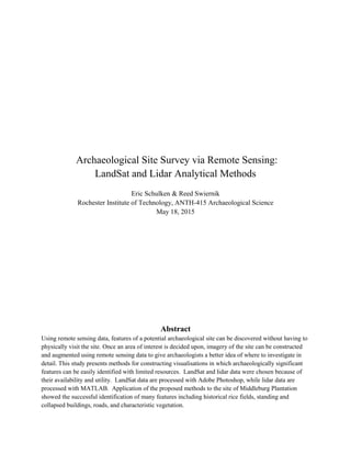
estimation for this can be made from a histogram of the Z components of a given data set or subset.
Vegetation cover should appear as a wide normal distribution, while the relatively flat ground below
should appear as a much narrower distribution below. The threshold should be set to the lowest height
value beyond the upper limit of the ground distribution (Figure 1). Although some residual elements of
the vegetation will persist, larger features below the tree cover should become more discernible. The

13
removal of vegetation also has the benefit of reducing the range of variability in the data, allowing for
more precision and definition to be granted in the visualization, i.e. higher color contrast.
Figure 1: Histogram of all point Z values (Top: full, Bottom: zoomed) used to select height threshold for
removing tree canopy from data.
One of the auxiliary problems that the software set out to solve was creating a contour map of an area.
This would allow for distinct features to be easily seen and identified, allowing archaeologists to isolate
areas of importance quickly. This contour map can then be pair with both the true color and false color
LandSat images to help interpret features.

14
4. Results
4.1 LandSat Composites
The LandSat image analysis can be split up into two distinct sections, creation of the true color
composite and creation of the false color composite. The true color composite image can provide a lot of
information about the site. The true color image of Middleburg, Figure 1 on the next page, identifies three
major parts to the property, the non-vegetated center area, the darker vegetated area surround the non-
vegetated area, and the lightly vegetated area that exists closer to the river boundary. These different main
areas will be used as seed areas of interest when looking at the false color LandSat images.
The false color images show us much more about the site. Figure 2 for example shows a strong
contrast from the wooded area around the house to the area bordering the river. This change from darker
pink to lighter pink indicates a change in both the type of vegetation that resides there as well as a soil
composition change. The change of vegetation goes from heavily vegetated near the house and main area
to almost no vegetation near the river. This area of low vegetation most like also has a different soil
composition, incapable of hosting the trees and other vegetation right next door.
Figure 3 reveals another odd relationship, visible in the bottom left hand corner. This image is
configured as bands 541 and when used in conjunction with 742 can give a better idea of the state of the
vegetation that is present at a site. In the plain RGB image, the area near the river shares a similar hue as
your follow the contour of the river. In Figure 3 this area in the bottom left corner is an active farm that is
more heavily irrigated than the section on the Middleburg property. This can be seen again in the change
from green to brown in Figure 3 and the change from green with blue in Figure 4. While these areas are
different between the two images, there is still similar shape and vegetation types. While the area in the
property next to Middleburg is damper on a whole, the RGB image and the rest of Figures 4 through 6
show that the areas are largely made up of the same or similar vegetation.
Figure 5 provides a high contrast view of non-vegetated areas that could be of interest. In this
region, vegetated areas can become overgrown and unnavigable. This view of our site area shows distinct
differences between different areas of vegetation and their relation to non-vegetated areas.
Figure 6 reveals heavy contrast with areas of water and can be used to find streams and bodies of water in
the area of interest. In this image we can clearly see the body of water near the main house. This can also
be seen in Figure 2 in the center of the shot. The other notable difference in this photo is the difference in
water saturation that can be observed in the area near the river.

15
Figure 1: True color RGB Figure 2: False color 432
Figure 3: False color 541 Figure 4: False color 742
Figure 4: False color 543 Figure 6: False color 453

16
4.2 Lidar Visualizations
Lidar visualizations were constructed with two goals: to detect remnants of agricultural activity--
namely rice fields--and to detect standing or collapsed structures. Visualizations were predominantly
made using mesh plots. Mesh plots proved to be better suited for visualizing buildings, while contour
plots were better for identifying rice fields near the river.
Figure 1: Lidar mesh plot of four square miles and a spatial resolution of 10 feet, with Middleburg
Plantation centrally located. The avenue of oaks is discernible, as are the earthen banks surrounding
former rice fields along the river.

17
Figure 2: Contour plot of the same data used for Figure 1 and contour separation of 1.5 feet. Surrounding
borders of rice fields very clearly visible.
Rice fields can be seen in both Figure 1 and Figure 2, though they become much more apparent in
Figure 2. The distinction between former rice fields and unaltered marshland is the presence of earthen
works surrounding the fields. These were designed to regulate the supply of water to the field. The
borders of the fields observed in Figure 2 align closely with those shown in a historical map of the
plantation (Appendix I: Figure 1) as well as the LandSat data shown in Section 4.1. The small island

18
where the Storehouse was located according to the map is also visible in Figure 2. This is one example of
smaller entities that are visible through Lidar data that are unable to be seen in LandSat data.
Figure 3: Lidar mesh plots of the Plantation House and grounds with a spatial resolution of 1 foot. The
left image shows all data, while the right shows the data with any points above 31 feet removed
Figure 3 was used to define smaller subsets of the data to examine in fine detail. Building
locations are apparent in the left-hand image, while the foundations of the stable can be seen in the right-
hand image. Neither of these features are able to be made out in the LandSat data. While the general
location of these structures can be inferred by the area of decreased vegetation, the structures themselves
cannot be determined. The right-hand image highlights small changes in elevation indicative of roads,
paths and ditches. Such features are more likely to be modern than archaeological at this site, though the
ability to detect such features could be of greater significance in other applications. A three dimensional
view of the same dataset as Figure 3 can be found in Appendix III: Figure 1.

19
Figure 4: Mesh plot of the Plantation House compared to a photograph. Spatial resolution: 0.5 feet.
Much of the detail of the Main House and surrounding buildings was captured in the Lidar data.
The hipped main roof, front porch roof and rear roof are all distinct, with pitches closely matching
photographs. The two chimneys are also represented in the data. Even the bush on the right side of the
house in the photograph in Figure 4 is represented in the mesh plot of the Lidar data. This close amount of
detail can be seen across all of the structures throughout the property.

20
Figure 5: Mesh plot of the Kitchen compared to a photograph. Spatial resolution: 0.5 feet.
Figure 6: Mesh plot of the Commissary compared to a photograph. Spatial resolution: 0.5 feet.

21
Figure 7: Mesh plot of the Stable location with points above 31 feet removed. Bottom image shows an
overlay of the shape and orientation of the Stable taken from Appendix I: Figure 2. Spatial resolution: 0.1
feet.

22
As in Figure 4, fine detail such as the chimney is represented in Figure 5. Distortions do occur
due to an overhanging tree. As such, Figure 6 shows the most accurate representation of any of the three
standing structures thanks to its isolation from vegetation. In figures 4, 5, and 6 it is clear that the
dimensions and proportions of the Lidar visualizations closely match those of the photographs.
Perhaps the most archaeologically relevant visualization is that of Figure 7. Attention was called
to this area thanks to the feature in the shape of a right angle, or what has been identified as the southern
corner of the Stable. The location and orientation of this corner were shown to be a near match with the
site map (Appendix I: Figure 2). The overlay in Figure 7 allows for further interpretation of features,
though it must be noted that any features in the upper section of the mesh plot (where vegetation was
removed) could be artifacts of the vegetation, rather than actual surface features.
Unfortunately, due to heavy tree cover, the storage house is unable to be seen. This is one of the
main weaknesses of the Lidar data. Through the use of the historical map in Appendix 1, Figure 1, the
storage rooms position is able to be placed in the rice fields adjacent to the river. This location can be
seen in the true color image of the area adjacent to the river and further magnified in Figure 8 of this
section. With the trees removed artificially from the image, there is a small area of similar elevation that
could possibly have been the location for the foundation for the original building, which can be seen in
Appendix 3, Figure 10. While the spatial resolution of the data is much better than that of the LandSat
images, neither will be able to fully inspect an element like the storage house as there is too much
environmental interference.
Figure 8: Aerial view of Storehouse location.

23
5. Conclusion
The methods that were developed in this study were able to successfully identify the major
features found in the historical map of Middleburg Plantation (Appendix I: Figure 1). Augmentation of
the relatively low resolution LandSat data with Lidar data allowed for greater certainty to be given to
interpretations of the data. On its own, Lidar data was shown to be useful for surveying standing and
collapsed buildings as well as roads and paths.
The most significant limitation of LandSat data is its low spatial resolution. Though this issue is
circumvented by the use of Lidar data, such data may not be available for all areas of archaeological
interest. The handling of Lidar data in Matlab was another limitation. Visualizations of large areas could
be constructed by first reducing the spatial resolution of the data. It would be advantageous to be able to
visualize an entire dataset at full resolution because it would eliminate the need to specify small areas to
investigate at full resolution. Smaller features that may be visible at full resolution may disappear at the
reduced resolution, meaning they would get overlooked with the current method. A computer or
computer cluster with more collective resources would be needed to run Matlab while data were being
processed. For reference, the four square mile dataset used to create Figures 1 and 2 in Section 4.2
initially contained approximately 25 million individual data points. The most resource intensive
operation was fitting the points to the mesh.
Further study could be taken in several directions. The methods described in this study could be
improved by making the implementation more user-friendly. In terms of the Lidar data, this would mean
giving the user the option to select a dataset and then an area of focus, rather than having to make changes
within the script to do so. In order to improve the rigor of the developed methods, it would be prudent to
apply them to a new area of study. This would allow for an assessment of how local conditions affect
results. The methods developed for processing and visualization of Lidar data could easily be adapted to
suit other archaeological pursuits. As seen in Figure 3 in Section 4.2, rudimentary removal of vegetation
can easily highlight roads and paths.

24
References
Agapiou, A., Alexakis, D. D., Sarris, A., Hadjimitsis, D. G. “Orthogonal Equations of Multi-Spectral
Satellite Imagery for the Identification of Un-Excavated Archaeological Sites” Remote Sensing.
5(12) (2013): 6560-6586. DOI:10.3390/rs5126560
Barnes, Jodi A. “What is Archaeology? Or What Does Landscape Have to Do with It?” South Carolina
Department of Archives and History. n.d.
Crutchley, S. “The Light Fantastic: Using Airborne LiDAR in Archaeological Survey” International
Society for Photogrammetry and Remote Sensing, 38, Part 7B. (July 2010). ISPRS TC VII
Symposium – 100 Years ISPRS, Vienna, Austria
Lasaponara, R., and Masini, N. “A review of satellite data processing methods applied in archaeological
context” Remote Sensing for a Changing Europe. (2009): 522-529. DOI:10.3233/978-1-58603-
986-8-522
Liew, S.C., "Principles of Remote Sensing." Centre for Remote Imaging, Sensing and Processing,
CRISP. Accessed May 18, 2015. http://www.crisp.nus.edu.sg/~research/tutorial/opt_int.htm.
“Middleburg” Digital Archaeological Archive of Comparative Slavery. 2015.
http://www.daacs.org/sites/middleburg/
“Middleburg Plantation - Huger - Berkeley County” South Carolina Plantations. 2014. http://south-
carolina-plantations.com/berkeley/middleburg.html
Morehart, Christopher T. “Mapping ancient chinampa landscapes in the Basin of Mexico: a remote
sensing and GIS approach” Journal of Archaeological Science. 39 (2012): 2541-2551
Quinn, J. "Band Combinations." Portland State University. 2001. Accessed May 18, 2015.
http://web.pdx.edu/~emch/ip1/bandcombinations.html.
Roberto, V., and Hofer, M., “Theia: Multispectral Image Analysis and Archaeological Survey”
Dipartimento di Matematica e Informatica, Norbert Wiener Center, University of Udine, Italy.
2009.
Vis, Benjamin N. “Report on the use of Matlab in analysing LiDAR data” Leiden University. July 2007.
Warmerdam, Frank. "TIFF Library and Utilities." LibTIFF. Accessed May 17, 2015.
http://www.remotesensing.org/libtiff/.

25
Appendix I - Additional Images
Figure 1: Map of Middleburg Plantation adapted from a 1786 plat (“Middleburg” 2015)

26
Figure 2: Map of excavation trenches (since filled) as well as current and former building locations
(“Middleburg” 2015)

27
Figure 3: The Main House in 2010 (Google Maps Panoramio)
Figure 4: The Kitchen in 1986 (“Middleburg” 2015)

28
Figure 5: The Commissary with location of Stable in background in 2010 (Google Maps Panoramio)

29
Appendix II - LandSat Data
Figure 1: Uncorrected image of the larger area surrounding the Middleburg Plantation.

30
Figure 2: True color image covering the larger area around the Middleburg Plantation.

31
R, G, B Description
3,2,1 The "natural color" band combination. Because the visible bands are used in this
combination, ground features appear in colors similar to their appearance to the human
visual system, healthy vegetation is green, recently cleared fields are very light,
unhealthy vegetation is brown and yellow, roads are gray, and shorelines are white. This
band combination provides the most water penetration and superior sediment and
bathymetric information.
4,3,2 The standard "false color" composite. Vegetation appears in shades of red, urban areas
are cyan blue, and soils vary from dark to light browns. Ice, snow and butts are white or
light cyan. Coniferous trees will appear darker red than hardwoods. Provides high
contrast and allows for large feature definition.
7,4,2 This combination provides a "natural-like" rendition, while also penetrating atmospheric
particles and smoke. Healthy vegetation will be a bright green and can saturate in seasons
of heavy growth, grasslands will appear green, pink areas represent barren soil, oranges
and browns represent sparsely vegetated areas. Dry vegetation will be orange and water
will be blue. Sands, soils and minerals are highlighted in a multitude of colors.
5,4,1 This will look similar to the 7 4 2 combination in that healthy vegetation will be bright
green. Water penetration is also much more readily apparent and can be seen in the blue
saturated areas.
5,4,3 This combination provides the user with a great amount of information and color
contrast. Healthy vegetation is bright green and soils are mauve. While the 7 4 2
combination includes TM 7, which has the geological information, the 5 4 3 combination
uses TM 5 which has the most agricultural information. Since we are surveying a
agricultural area, this view can show stark differences between areas.
4,5,3 This combination of near-IR (Band 4), mid-IR (Band 5) and red (Band 3) offers added
definition of land-water boundaries and highlights subtle details not readily apparent in
the visible bands alone. Inland lakes and streams can be located with greater precision
when more infrared bands are used. With this band combination, vegetation type and
condition show as variations of hues (browns, greens and oranges), as well as in tone.
The 4,5,3 combination demonstrates moisture differences and is useful for analysis of
soil and vegetation conditions. Generally, the wetter the soil, the darker it appears,
because of the infrared absorption capabilities of water.
Table 1: A modified version of the model by Quinn

32
Appendix III - Lidar Data
Figure 1: Aerial view of the plantation house and grounds looking down the avenue of oaks towards the
house. Bottom view was created by removing all data above 32 feet. Ditches on either side of the main
drive become clearly visible.

33
Figure 2: Zoomed view looking north. Main House, Kitchen, and Commissary all visible.

34
Figure 3: Aerial view of Plantation House

35
Figure 4: Aerial view of Kitchen with a large live oak tree in the background.

36
Figure 5: Aerial view of the Commissary.
Figure 6: Aerial view of Stable location. View obscured by trees.

37
Figure 7: Aerial view of Stable location with trees removed.
Figure 8: Aerial view of the location of the main block of archaeological trenches.

38
Figure 9: Aerial view of the location of the main block of archaeological trenches with trees removed. No
evidence of trenches. The lateral ridges that are visible appear to be artifacts of the lidar sensor sweeping
horizontally, as they appear in all regions of the data.
Figure 10: Birdseye view of Storehouse location with vegetation removed. Possible evidence of a
collapsed structure in a raised area in the center of the island.

39
Appendix IV - MATLAB Script
% LiDAR .las data plotting tool
% Rochester Institute of Technology
% ANTH-415 Archaeological Science
% Spring 2015 Final Project
% Reed Swiernik & Eric Schulken
% Plot all data for survey area
% Read Data Files and Stitch together
a = lasdata('SC_BerkeleyCo_2009_000928.las'); % TL
b = lasdata('SC_BerkeleyCo_2009_000932.las'); % BL
c = lasdata('SC_BerkeleyCo_2009_000930.las'); % TR
d = lasdata('SC_BerkeleyCo_2009_000870.las'); % BR
x=[a.x;b.x;c.x;d.x]; y=[a.y;b.y;c.y;d.y]; z=[a.z;b.z;c.z;d.z];
clear a; clear b; clear c; clear d;
mx = min(x):10:max(x); my = min(y):10:max(y);
[X Y]=meshgrid(mx,my); Z = griddata(x,y,z,X,Y);
clear x; clear y; clear z;
figure(1)
mesh(X,Y,Z); view(2); colorbar; axis image
% END
% LiDAR .las data plotting tool
% Rochester Institute of Technology
% ANTH-415 Archaeological Science
% Spring 2015 Final Project
% Reed Swiernik & Eric Schulken
% Plot Main house and grounds, focus on individual buildings
% Specify and import data
c = lasdata('SC_BerkeleyCo_2009_000928.las');
R = 0.5; % Mesh resolution in feet
x=c.x; y=c.y; z=c.z;
dat = [x y z];
%% House
% Define subset to examine
xL = 2354100;
xR = 2354230;
yB = 455660;
yT = 455750;
% Reduction of data to specified subset
F1 = find(dat(:,1)<xR); B = dat(F1,:);
F2 = find(B(:,1)>=xL); C = B(F2,:); F3 = find(C(:,2)<=yT);

40
D = C(F3,:); F4 = find(D(:,2)>yB); reduceddat=D(F4,:);
x = reduceddat(:,1); y = reduceddat(:,2); z = reduceddat(:,3);
mx = min(x):R:max(x); my = min(y):R:max(y);
figure(2)
mesh(X,Y,Z); view(2); colorbar; rotate3d on; view(2); axis image
title('Main House'); xlabel('Easting (ft)'); ylabel('Northing (ft)');
zlabel('Height above Reference (ft)');
%% Kitchen
xL = 2354130;
xR = 2354200;
yB = 455750;
yT = 455820;
figure(3)
title('Kitchen'); xlabel('Easting (ft)'); ylabel('Northing (ft)');
%% Comissary
xL = 2354450;
xR = 2354550;
yB = 455920;
yT = 456000;
figure(4)
title('Comissary'); xlabel('Easting (ft)'); ylabel('Northing (ft)');
%% Stable

41
xL = 2354600;
xR = 2354800;
yB = 456060;
yT = 456200;
figure(5)
title('Stable'); xlabel('Easting (ft)'); ylabel('Northing (ft)');
length = size(x);
for i=1:length(1)
if z(i)>31
x(i)=xL;
y(i)=yT;
z(i)=28;
end
end
[X Y]=meshgrid(mx,my);
Z = griddata(x,y,z,X,Y);
figure(6)
mesh(X,Y,Z); view(2); colorbar
% axis ([2353800 2355000 455000 456300 6 31])
rotate3d on
axis image
title('Stable Without Trees');
xlabel('Easting (ft)'); ylabel('Northing (ft)');
%% Trenches
xL = 2354300;
xR = 2354450;
yB = 455800;
yT = 455930;

42
figure(7)
title('Excavation Trench Area');
% Remove data above threshold
length = size(x);
for i=1:length(1)
if z(i)>31
x(i)=xL;
y(i)=yT;
z(i)=28;
end
end
figure(8)
rotate3d on
axis image
title('Trenches without Trees');
%% Overall
xL = 2353800;
xR = 2355500;
yB = 455000;
yT = 456300;
figure(9)
title('Plantation House and Grounds')

43
% Histogram for deterining threshold
figure(16)
hist(z,200);
% Remove data above threshold
length = size(x);
for i=1:length(1)
if z(i)>31
x(i)=xL;
y(i)=yT;
z(i)=28;
end
end
figure(10)
% axis ([2353800 2355000 455000 456300 6 31])
rotate3d on
axis image
title('Plantation House and Grounds without Trees');
% END

Schulken_Swiernik-Archaeological_Site_Survey

Recommended

Recommended

More Related Content

What's hot

What's hot (20)

Viewers also liked

Viewers also liked (8)

Similar to Schulken_Swiernik-Archaeological_Site_Survey

Similar to Schulken_Swiernik-Archaeological_Site_Survey (20)

Schulken_Swiernik-Archaeological_Site_Survey