beven 2001.pdf

Equi®nality, data assimilation, and uncertainty estimation in
mechanistic modelling of complex environmental systems using
the GLUE methodology
Keith Beven*, Jim Freer
Institute of Environmental and Natural Sciences, Lancaster University, Lancaster LA1 4YQ, UK
Received 9 December 1999; revised 22 May 2000; accepted 25 May 2000
Abstract
It may be endemic to mechanistic modelling of complex environmental systems that there are many different model
structures and many different parameter sets within a chosen model structure that may be behavioural or acceptable in
reproducing the observed behaviour of that system. This has been called the equi®nality concept. The generalised likelihood
uncertainty estimation (GLUE) methodology for model identi®cation allowing for equi®nality is described. Prediction within
this methodology is a process of ensemble forecasting using a sample of parameter sets from the behavioural model space, with
each sample weighted according to its likelihood measure to estimate prediction quantiles. This allows that different models
may contribute to the ensemble prediction interval at different time steps and that the distributional form of the predictions may
change over time. Any effects of model nonlinearity, covariation of parameter values and errors in model structure, input data or
observed variables, with which the simulations are compared, are handled implicitly within this procedure. GLUE involves a
number of choices that must be made explicit and can be therefore subjected to scrutiny and discussion. These include ways of
combining information from different types of model evaluation or from different periods in a data assimilation context. An
example application to rainfall-runoff modelling is used to illustrate the methodology, including the updating of likelihood
measures. q 2001 Elsevier Science B.V. All rights reserved.
Keywords: TOPMODEL; Maimai catchment; Rainfall-runoff modelling; Parameter conditioning; Prediction uncertainty; GLUE
1. Equi®nality in modelling complex
environmental systems
It will be argued in this paper that, given current
levels of understanding and measurement technolo-
gies, it may be endemic to mechanistic modelling of
complex environmental systems that there are many
different model structures and many different para-
meter sets within a chosen model structure that may
be behavioural or acceptable in reproducing the
observed behaviour of that system. Hornberger and
Spear (1981), whose work originally inspired what
follows here, noted that this is not simply a problem
of identifying a correct or optimal model given
limited data. Indeed, to focus attention on a rejection
of the concept of the optimal model in favour of multi-
ple possibilities for producing simulations that are
acceptable simulators in some sense, this idea has
been called elsewhere equi®nality (Beven, 1993,
1996a,b). Equi®nality should not be a surprising
concept. It can often be argued on grounds of physical
Journal of Hydrology 249 (2001) 11±29
0022-1694/01/$ - see front matter q 2001 Elsevier Science B.V. All rights reserved.
PII: S0022-1694(01)00421-8
www.elsevier.com/locate/jhydrol
* Corresponding author. Fax: 144-1524-593-985.
E-mail address: k.beven@lancaster.ac.uk (K. Beven).

theory that there should be suf®cient interactions
among the components of a system that, unless the
detailed characteristics of these components can be
speci®ed independently, many representations may
be equally acceptable.
The idea of searching for a single optimal represen-
tation of reality is, however, very strong in environ-
mental science. It is part of the normal working
paradigm that research should lead to a realistic
description of the real processes and characteristics.
It is rarely considered that such a description may not
be possible or uniquely identi®able despite the fact
that for many systems the working descriptions are
wrong and are known to be wrong (see the analysis
of Morton, 1993), and that many system components
may not be accessible to adequate observation given
current measurement technologies (particularly, as in
hydrology, where much of the active components of
the system are below the ground surface). Thus,
modelling of complex environmental systems
generally involves the indirect identi®cation of
model components or parameters by posing an inverse
problem. Often, such inverse problems involve
multiple parameters and observations that are only
indirectly related to the parameters of interest, or
which may be at different scales to the variables and
parameters used in the model calculations. A particu-
lar problem occurs in distributed predictions where
the use of global parameters will result in error in
predicting local responses at points with unique
characteristics (Beven, 2000). In such cases, the
inverse problem will not be well posed and identi®ca-
tion of an optimal solution will be neither easy nor
robust to a change of data set. This has been the
subject of considerable study in the groundwater
literature (e.g. McLaughlin and Townley, 1996), but
has not been much studied in the more dif®cult case of
distributed rainfall-runoff modelling.
This, in itself, should not be suf®cient to reject the
idea of an optimal model but a search of the feasible
model structure and parameter space will commonly
reveal many behavioural models with similar levels of
performance in reproducing observational data. The
concept of the optimal model must then be seriously
questioned. Such searches have, until recently, not
been computationally possible and remain computa-
tionally demanding or impossible for many complex
models, such as long runs of global coupled ocean±
atmosphere circulation models. Thus, it has only
recently been possible to recognise the ubiquitous
nature of the equi®nality problem. Simulations of a
variety of different systems, however, have now
demonstrated that even moderate levels of model
complexity start to reveal equi®nality. This has been
shown for rainfall-runoff models (Beven and Binley,
1992; Duan et al., 1992; Beven, 1993; Romanowicz et
al., 1994; Freer et al., 1996; Fisher et al., 1997; Pin
Äol
et al., 1997; Franks et al., 1998; Lamb et al., 1998;
Dunn et al., 1999; Beven, 2001; Beven and Freer,
2001); ¯ood frequency and inundation models
(Romanowicz et al., 1996; Romanowicz and Beven,
1998; Aronica et al., 1998; Cameron et al., 1999);
river dispersion models (Hankin et al., 1998); soil±
vegetation±atmosphere models (Franks and Beven,
1997a,b, 1999; Franks et al., 1999); groundwater
¯ow and transport models (Buckley et al., 1995);
and soil geochemical models (Zak et al., 1997; Zak
and Beven, 1999; Schulz et al., 1999).
2. Equi®nality as a working paradigm
One implication of rejecting the concept of an
optimal parameter set and accepting the concept of
equi®nality is that the uncertainty associated with
the use of models in prediction might be wider than
has hitherto be considered, since if there are several
(many?) different acceptable model structures or
many acceptable parameter sets scattered throughout
the parameter space, all of which are consistent in
some sense with the calibration data, the range of
any predicted variables is likely to be greater than
might be suggested by a linearised analysis of the
area of parameter space around the `optimum'. This
suggests that the predictions of all the acceptable
models (from here on model will be used to mean a
particular model structure/parameter set combination)
should be included in the assessment of prediction
uncertainty, weighted by their relative likelihood or
level of acceptability. Such an approach allows the
nonlinearity of the response of acceptable model
using different parameter sets to be taken into account
in prediction.
This appears to lead quite naturally to a form of
Bayesian averaging of models and predictions, in
which prior distributions of models are assessed in
K. Beven, J. Freer / Journal of Hydrology 249 (2001) 11±29
12

terms of some likelihood measure relative to the
observations and a posterior distribution calculated
that can then be used in prediction. This is the basis
of the generalised likelihood uncertainty estimation
(GLUE) methodology proposed by Beven and Binley
(1992), which has now been used in a variety of
modelling contexts with a variety of likelihood
measures in the applications noted above. Updating
of the model likelihood distributions as new calibra-
tion data become available is handled easily within
the Bayesian framework.
In the GLUE methodology, some prior information
about feasible ranges of parameter values is used to
control the generation of independent random
parameter sets for use in each model. An input
sequence is used to drive each model and the results
are compared with the available calibration data. The
model simulations may have either a deterministic or
a stochastic dependence on the parameters and input
data, but the methodology has to date been primarily
used with deterministic models. A quantitative
measure of performance or likelihood measure is
used to assess the acceptability of each model based
on the modelling residuals.
Effectively, each model run represents a sample on
the response surface of the likelihood measure within
the model space. The comparison of models in Fig.
1a±c represents a projection of the sampled response
surface onto a single parameter axis. Each dot on these
plots represents the results of a single realisation of a
multiple parameter model, expressed in terms of a
single summary likelihood measure, here based on a
sum of squared errors criterion. The large number of
models giving high values of the likelihood measure is
an expression of the equi®nality in modelling this data
set. In this case, the large number of good or beha-
vioural models are from different parameter sets
within a single model structure. Extension to multiple
competing model structures is simple, provided that a
directly comparable likelihood measure may be used,
which only requires that the different model structures
included in the analysis must predict a variable that
can be compared with a common set of available
observations or other consistent information.
As projections, Fig. 1a±c do not reveal any obvious
structure in the response surface arising from inter-
action between different parameter values. In general,
of course, such interactions may be of great interest in
guiding the modeller as to the sensitivity of the predic-
tions to different combinations of parameter values
and to where model reformulation and simpli®cation
might be appropriate. However, in the present context
it is suf®cient to note that it is the set of parameter
values that is important in giving either good or poor
performance, and that it is the set of models giving
good performance that is of greatest interest and that
is spread across the ranges of the individual para-
meters.
Other performance criteria have also been
suggested and proposed (Beven and Binley, 1992)
including fuzzy possibility measures (Aronica et al.,
1998; Franks and Beven, 1998; Franks et al., 1998)
and likelihood functions based on speci®c error
models (Romanowicz et al., 1994, 1996; Romanowicz
and Beven, 1998). The choice of likelihood measure is
an important issue in this methodology.
3. The choice of an appropriate likelihood measure
Many environmental modelling problems involve
the modelling of time series or spatial patterns of
observations, sometimes a single observed output or
state variable, sometimes multiple observations at
each time step. The model may involve multiple para-
meters and multiple model state variables not all of
which will be measured or, indeed, observable. The
model residuals, or errors, when compared with the
observations will often have a complex structure.
Experience suggests that they may show non-station-
ary bias, non-stationary variance, non-stationary
skewness, and autocorrelation over one or more
time steps.
However, for an initial analysis, consider the
following traditional approach to likelihood estima-
tion. We assume, perhaps after a suitable transforma-
tion, an error model of additive type, with Gaussian
autocorrelated errors. Let Zt be the observed time
series, Mt(Q,Y) the model output at time t, given the
times series of inputs Y and the set of parameter values
Q, so that
Zt ˆ Mt…Q; Y† 1 et…F† …1†
where et(F) represents the error model with para-
meters F. For a nth order Gaussian autoregressive
K. Beven, J. Freer / Journal of Hydrology 249 (2001) 11±29 13

14

model AR(n)
et ˆ m 1
X
n
iˆ1
ai…et21 2 m† 1 s2
dt …2†
where dt should be N[0,1]. For the simplest ®rst order
correlation case, F ˆ …m; s; a† the likelihood function
is then given by
L…ZuQ; F; Y† ˆ …2ps2
†2t=2
…1 2 a2
†1=2
£ exp
"
2
1
2s2
(
…1 2 a2
†…e1 2 m†2
1
X
t
tˆ2
…et 2 m 2 a…et21 2 m††2
)#
…3†
where t is the number of time steps in the simulation.
Note that if the quantities Zt and Mt(Q,Y) are taken to
be log transformed observations and model outputs,
respectively, then this same model can be used for
multiplicative errors, which allows for the effects of
an error variance that changes with the magnitude of
the observation (one possible heteroscedastic case).
Transformations, such as Box±Cox transforms, of
the observed and predicted variables may also be
used to stabilise the error variances (Box and Cox,
1964).
It is, of course, possible to use more complex like-
lihood functions but this will serve for illustrative
purposes. Mechanistic environmental model simula-
tions may involve a large number of time steps. The
magnitude of the likelihood function then tends to be
dominated by the ®rst bracketed term on the RHS,
…2ps2
†2t=2
, essentially the error variance raised to a
large negative power. The remaining terms correct for
any model bias effects and the reduction in informa-
tion content of the errors at successive time steps
resulting from the correlation of the residuals. The
result of t/2 being very large is to greatly accentuate
the peak values of likelihood in the parameter space.
This is, of course, an advantage if an optimum is being
sought, since essentially only the simulations having
the minimum variance will survive an operation that
may involve powers of hundreds or even thousands.
Thus, the concept of an optimum parameter set neces-
sarily survives in this framework, and in ®nding the
maximum likelihood solution the calculations can be
carried out in log space so that t/2 becomes a multi-
plier and the numerical problems of using such large
powers are avoided. To some extent this obscures the
fact that, because of using such large powers, there is
only information in the likelihood surface in the
immediate vicinity of the `optimum'. An example of
such a transformation, in this case with the shaping
factor N ˆ 30 (see Table 1 (1b)), is shown in Fig. 1d±f.
This would suggest, therefore, that the parameters
are extremely well identi®ed. However, it is clear
from Fig. 1a±c that this might be a misleading impres-
sion. There are many simulations from different parts
of the parameter space that, on the basis of the error
variance alone, are virtually indistinguishable from
one another. These are clearly two extreme cases,
one of which may overestimate parameter identi-
®ability, the other may underestimate parameter
identi®ability. However, one implication of the differ-
ence between them is that, because of the extreme
transformation inherent in Eq. (3) the maximum
likelihood parameter set may not survive the use of
a different calibration data set or sub-set.
In addition, once the maximum likelihood model
has been found, the calculation of uncertainty in the
predictions, and estimates of the variance and covar-
iance of the parameters, generally involves an
assumption of local linearity of the log-likelihood in
the neighbourhood of the optimum. However, one of
the features of environmental models is that they are
often highly nonlinear. In this case it may be neces-
sary to evaluate the complete likelihood surface
(including the error parameters F) to assess the
uncertainty in the predictions properly, by means of
evaluating likelihood ratios, parametric bootstrapping
or Monte Carlo Markov Chain methods (e.g.
Tarantola, 1987; Kuczera and Parent, 1998). In differ-
ent parts of this parameter space, it may be that the
calculated residuals will not have the same assumed
structure, even if that is the case at the maximum
likelihood point. Also, remember that in this analysis
we have actually added (at least) three additional
parameters of the error model, that could result in
the error model compensating for de®ciencies in the
Fig. 1. Dotty plot of likelihood values for selected TOPMODEL parameters from Monte Carlo simulations of the Maimai catchment condi-
tioned on the 1985a discharge period (a±c) using (1b) of Table 1 with N ˆ 1; d±f using (1b) of Table 1 with N ˆ 30).

mechanistic model such that a simulation with a
consistent bias might have a better pro®le likelihood
value than an unbiased simulation, since Eq. (3) does
not penalise against such a bias when applied locally
in the response surface.
This situation arises because the likelihood function
implicitly assumes that there is a true model of the
observations so that the appropriate error model for
the residuals is easily evaluated. This is not often the
case in environmental modelling. Errors arise due to
model structure, errors in boundary and forcing
conditions and error in the observations, with which
the model is compared. It may be very dif®cult indeed
to separate these sources of error. The likelihood
function is de®ned as the likelihood of the observa-
tions, given the model and error model. In environ-
mental modelling we are generally more interested in
the likelihood of the mechanistic model as a simulator
of the system given, and conditional on, the (non-
error-free) input data and (non-error-free) observa-
tions.
We are still, however, interested in the combination
of states of information that underlies the likelihood
principle. This suggests a more generalised approach
to likelihood based parameter estimation, in which it
is the likelihood of different models (parameter sets
and/or structures) that is being investigated.
4. Generalised likelihood uncertainty estimation
Beven and Binley (1992) pointed out that, viewed
in this light, many different likelihood measures might
be appropriate in a given application setting. The aim
is to assess the performance of different models in a
way that allows different measures (calculated for
different variables or different periods) to be
combined in a suitable way. They outlined a number
of ways of formulating both likelihood measures and
ways of combining likelihood measures, including the
following form of Bayes equation:
L‰M…Q†Š ˆ L0‰M…Q†ŠLT ‰M…QuYT ; ZT †Š=C …4†
where L0[M(Q)] is a speci®ed prior likelihood for the
model M(Q) with parameter vector, Q,
LT ‰M…QuYT ; ZT †Š is a likelihood measure calculated
for the model over period T with input vector YT and
observed variable vector ZT , and C is a scaling
constant. Note that it is now the likelihood of the
model (parameter set and/or structure), M…Q†, that is
being assessed, rather than the value of an observation
or of the individual parameters. Application of Eq. (4)
implies that the values of the likelihood measures
calculated for different models can be considered
independent. Hence the attempt in traditional likeli-
hood measures to achieve a residual series dt that is
white, and that can be tested for its whiteness as a test
of the error model used.
In general such orthogonality cannot be assured for
mechanistic environmental models. However, by
using model parameter sets that are chosen indepen-
dently from some speci®ed distributions, indepen-
dence in sampling the likelihood surface can be
assured, at least within a chosen parameter metric.
This is easily done in a Monte Carlo sampling
framework using either an importance sampling tech-
nique (so that the shape of the response surface is
represented by the density of sampling and each
model simulation is given equal weight in forming a
distribution of predictions) or a uniform sampling
technique (so that each model simulation is associated
with a likelihood value re¯ecting the shape of the
16
Table 1
Example likelihood measures used in GLUE applications, where F ˆ …m; s; a† and t are de®ned in the text; s2
e is the error variance; s2
0 is the
variance of the observations. M…QiuYT ; ZT † indicates the ith model, conditioned on input data YT and observations ZT
Based on autocorrelated Gaussian error model
(Romanowicz et al., 1994, 1996)
L‰ZT uQ; F; YT Š ˆ …2ps2
†2t=2
…1 2 a2
†1=2
exp‰2…1=2s2
†{…1 2 a2
†…e1 2 m†2
1
Pt
tˆ2…et 2 m 2 a…et21 2 m††2
}Š
(1)
Based on inverse error variance with shaping factor N
(Beven and Binley, 1992)
L‰M…QuYT ; ZT †Š ˆ …s2
e †2N
(1a)
Based on Nash and Sutcliffe ef®ciency criterion with
shaping factor N (Freer et al., 1996)
L‰M…QuYT ; ZT †Š ˆ …1 2 s2
e =s2
0 †N
for s2
e , s2
0 (1b)
Based on exponential transformation of error
variance with shaping factor N (Freer et al., 1996)
L‰M…QuYT ; ZT †Š ˆ exp…2Ns2
e † (1c)

response surface). Both are ways of characterising the
response surface in the model parameter space. Appli-
cations of GLUE have used the latter, trading off the
inef®ciency of uniform sampling against ease of
implementation and minimal assumptions about the
shape of the response surface. The results of each
model can then be compared with the data and a like-
lihood measure calculated, so that Eq. (4) can then be
applied in the form
L‰M…Qi†Š ˆ L0‰M…Qi†ŠLT ‰M…QiuYT ; ZT †Š=C …5†
where M…Qi† indicates the ith model. If appropriate,
the likelihood LT ‰M…QiuYT; ZT †Š might be of the form
of a measure de®ned by the likelihood function of
Eq. (3), but a more application oriented, rather than
error oriented, measure might be more appropriate,
particularly if the model is not a particularly good
representation of the data (as is often the case).
Examples of likelihood measures used in different
applications are given in Table 1. The likelihood
measure will re¯ect the performance of a particular
model, given the model nonlinearity and errors in
model structure, inputs and observations. Since the
likelihood measure value is associated with a para-
meter set, it will re¯ect all these sources of error
and any effects of the covariation of parameter values
on model performance implicitly. The only constraint
is that it should increase monotonically with increase
in model performance (however, that is de®ned) and
that model simulations that are considered as non-
behavioural should have a likelihood of zero. Equi-
®nality in model performance will be re¯ected
directly by different models having similar values of
the chosen likelihood measure.
Given a large enough sample of Monte Carlo simu-
lations, the range of likelihood weighted predictions
may then be evaluated to obtain prediction quantiles
at any time step. This is most easily done if the like-
lihood values are renormalised such that
PB
iˆ1 L‰M…Qi†Š ˆ 1, where M…Qi† now indicates the
ith behavioural Monte Carlo sample, so that at any
time step t
P… ^
Zt , z† ˆ
X
B
iˆ1
L‰M…Qi†u ^
Zt;i , zŠ …6†
where ^
Zt;i is the value of variable Z at time t simulated
by model M…Qi†. The prediction quantiles, P… ^
Zt , z†
obtained in this way are conditional quantiles: condi-
tioned on the inputs to the model; the model responses
for the particular sample of parameter sets used; the
choice of likelihood measure; and the observations
used in the calculation of the likelihood measure. In
such a procedure the simulations contributing to a
particular quantile interval may vary from time step
to time step, re¯ecting the nonlinearities and varying
time delays in model responses. It also allows for the
fact that the distributional characteristics of the like-
lihood weighted model predictions may vary from
time step to time step (sometimes dramatically, see
Freer et al., 1996). Note that Eq. (6) implicitly re¯ects
the fact that the independence in sampling the para-
meter sets does not imply independence of the
predicted variables of interest resulting from the simi-
lar (if not identical) input data and boundary condi-
tions used to force the model (Bernardo and Smith,
1994). Model outputs will tend to be correlated, even
for models judged to be non-behavioural.
If more than one period of data is available, Bayes'
equation (5); (Box and Tiao, 1973) can be reapplied to
update the likelihood weights on a parameter set by
parameter set basis, re¯ecting the independence of the
parameter sampling. The posterior from one applica-
tion of Eq. (5) becomes the prior for the next applica-
tion. The likelihood measures for a given parameter
set for the periods may be correlated, indeed it should
be hoped (if not necessarily expected) that if a model
performs well in one calibration period, it will
continue to perform well in other periods. If this is
not the case then its combined likelihood measure will
be reduced.
It is possible that, in combining two measures from
different observed variables during the same calibra-
tion period, there will be a correlation in model
performance against different variables, i.e. a model
that produces good simulations of one output variable
might equally produce good simulations of an
observable internal state variable (although it has to
be said that this does not necessarily follow in many
applications). A simple application of Eq. (5) to the
weights associated with each model separately will
be effectively ignoring this correlation. It will
have the desired effect that if a model produces
good simulations on both variables its likelihood
will be raised, if it does not, it will be lowered but
a fully rigorous application of Eq. (5) would

require a proper assessment of the information
content of each measure.
The choice of method of combining likelihood
measures may have implications for the choice of
the measure itself, in particular if it is required that
multiple combinations, for example of measures from
different periods of data, have the same result as
treating the data as a single continuous period
(where this is possible). Repeated application of Eq.
(5) would not lead to this end if, for example, the
likelihood measure was a linear function of the
inverse error variance for each separate period of
data. The successive multiplications would result in
the most recent period of data having the greatest
weight in the determination of the likelihoods after
resampling (which may, of course, give the desired
effect if the system is thought to be changing over
time). The use of a likelihood measure that is a
constant linear function of the inverse exponential of
the error variance, would result in an equivalence of
®nal posterior likelihood (Table 1, Eq. (1c)).
There are also other ways of combining likelihood
measures. As one example, the likelihood measures
may be re-interpreted directly as fuzzy possibility
measures so that the techniques of fuzzy union
(Table 2, Eq. (5b)) and fuzzy intersection (Table 2,
Eq. (5c)) could also be used. The value of additional
data in re®ning the likelihood measure distribution
associated with the parameter sets can be evaluated
using different uncertainty measures (see Beven and
Binley, 1992).
In essence, a generalised likelihood framework is
being proposed, in which a variety of likelihood
measures (including traditional likelihood functions)
could be used. The choice of likelihood measure, and
the way of combining likelihood measures, are
subjective but, clearly, reasonable choices should be
made for any particular application. An important
point to be made, however, is that the choices must
be made explicit so that the analysis can be repro-
duced at any time to check calculations, to compare
different model structures or the effects of using
different calibration variables etc. Being explicit,
they can also be the subject of discussion and justi®-
cation.
5. Generating parameter sets
The proposed methodology separates parameter
sampling, to ensure independence of chosen para-
meter sets, with likelihood evaluation. As such it
varies from much of the recent work in Monte Carlo
Markov Chain and similar techniques that attempt to
sample the parameter space according to likelihood
power, with the hope of making considerable savings
in computer time in de®ning the likelihood surface.
Such methods may work well when there is a well
de®ned surface, but for surfaces with lots of local
maxima or plateaux, the advantages may not be
great.
The shape of the response surface will, of course,
re¯ect the likelihood function used. The choice of a
likelihood measure, for example …2ps2
†2t=2
that is the
dominant term of Eq. (3) with t large, that emphasises
the peak will then be advantageous but only if the
resulting distributions of likelihood weighted predic-
tions are reasonable in comparison with the observa-
tions. Raising the peak likelihood, relative to other
values in the response surface, will generally have
18
Table 2
Examples of likelihood measure combination equations (before renormalisation), where v0 and v1 are weighting coef®cients for different
periods or different variables. M…QiuYT ; ZT † indicates the ith model, conditioned on input data YT and observations ZT
Bayes' multiplication (e.g.
Beven and Binley, 1992;
Romanowicz et al., 1994, 1996)
L‰M…Qi†Š / L0‰M…Qi†ŠL1‰M…Q1iuY1; Z1†Š (5)
Weighted addition (Zak et al.,
1997)
L‰M…Qi†Š / 40L0‰M…Qi†Š 1 41L1‰M…QiuY1; Z1†Š (5a)
Fuzzy union L‰M…Qi†Š / Min‰L0‰M…Qi†Š; L1‰M…QiuY1; Z1†ŠŠ (5b)
Fuzzy intersection L‰M…Qi†Š / Max‰L0‰M…Qi†Š; L1‰M…QiuY1; Z1†ŠŠ (5c)
Weighted fuzzy combination
(Aronica et al., 1998)
L‰M…Qi†Š / 40Min‰L0‰M…Qi†Š; L1‰M…QiuY1; Z1†ŠŠ 1 41Max‰L0‰M…Qi†Š; L1‰M…QiuY1; Z1†ŠŠ (5d)

the effect of narrowing the tails of the distributions of
predictions, perhaps in some cases too much to allow
the prediction limits to encompass many of the obser-
vations (e.g. Freer et al., 1996).
Thus the whole of the response surface may be of
interest. Getting an adequate de®nition of that surface
will be computationally expensive in high dimen-
sional parameter surfaces. Both uniform Monte
Carlo and Latin Hypercube sampling could be used
to obtain parameter sets that are distributed through-
out the parameter space and independent within that
metric. Only the feasible parameter range and the
scaling of the parameter axis must be speci®ed for
uniform sampling. Latin Hypercube sampling can be
used to generate minimally correlated parameter sets
in the case where there is some prior information
about parameter covariation. With anything more
than a small number of parameters, a large number
of samples will be required for a proper characterisa-
tion of the response surface.
Prior information about parameters may take a
number of forms. The ®rst would be some sense of
expected distribution and covariance of the parameter
values. Some parameter sets, within the speci®ed
ranges, may be known a priori as not being feasible
on the basis of past performance or mechanistic argu-
ments. Then each parameter set might be given a prior
likelihood (perhaps of zero): this need not change the
sampling strategy but does mean that if the prior like-
lihood is zero it will not be necessary to run the model
thereby saving computer time. It must be remembered
that any parameter values outside the speci®ed range are
being given an a priori likelihood of zero, even while it
will be commonly found that behavioural models may
be found right up to the edge of this range (see Fig. 1a, b
and many of the studies quoted above).
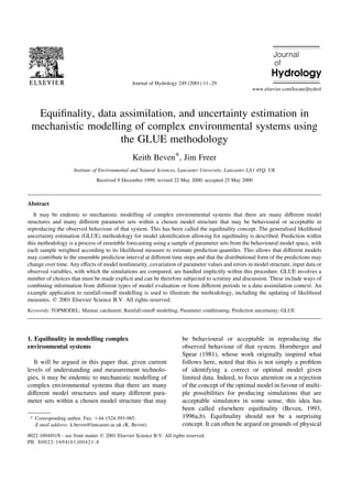
Fig. 2. Spatial distribution of the ln…a=tan b† topographic index for the Maimai M8 catchment, New Zealand.

There may also be some idea of the form of the
expected response surface. This might be used to
specify a different noninformative prior than the
uniform prior suggested above, for example to use a
prior that is conjugate with the expected posterior (see
Bernardo and Smith, 1994). Again, however, this need
not change the uniform sampling strategy, but each
parameter set would not be given a uniform prior like-
lihood in this case. Alternatively, much more ef®cient
sampling of the response surface might be achieved in
such cases using a Monte Carlo Markov Chain
(MCMC) algorithm or the structured tree algorithm
of Spear et al. (1994).
An interesting question arises when there are
measured values available of one, some or all para-
meter values in the model. In some (rare) cases it may
even be possible to specify distributions and covar-
iances for the parameter values on the basis of
measurements. These could then be used to specify
prior likelihood weights in the (still uniformly)
sampled parameter space. Although it is often the
case that such measurements are the best information
that we have about parameter values, there is,
however, no guarantee that the values measured at
one scale will re¯ect the effective values required in
the model to achieve satisfactory functional predic-
tion of observed variables (Beven, 1989; Beven,
1996b). It might then be possible to feed disinforma-
tion into the prior parameter distributions but the
repeated application of Eq. (5) or some other way of
combining likelihood measures should result in the
performance of the model increasingly dominating
the shape of the response surface, unless prior like-
lihood weights assigned as zero have wrongly
excluded some of the parameter space from consid-
eration. In some cases this will be obvious, such as
where initial results indicate that resampling of para-
meter sets beyond the prior speci®ed sampling ranges
should be carried out.
6. An example application: rainfall-runoff
modelling of the Maimai M8 catchment, New
Zealand, with the assimilation of successive
periods of data
The small Maimai M8 (3.8 ha) catchment is located
in the Tawhai State Forest, North Westland, South
Island, New Zealand. It has been the focus for a
variety of studies of hydrological processes (see
Rowe et al., 1994, and Brammer and McDonnell,
1996). The catchment has a mean annual gross preci-
pitation of 2600 mm, producing some 1550 mm of
runoff from 1950 mm net precipitation with little
seasonal variation. The catchment is underlain by a
compact early Pleistocene conglomerate, called the
Old Man Gravels, that is thought to be essentially
impermeable. Slopes in the catchment are short and
steep with a relief of 100±150 m. The soils are
spatially variable in depth (0.2±1.8 m) and hydraulic
conductivity, but are generally highly permeable. The
vegetation is a mixed evergreen forest with an under-
story of tree ferns and shrubs.
This wet environment and sloping terrain is a suita-
ble test environment for the rainfall-runoff model
TOPMODEL (Beven and Kirkby, 1979; Beven et
al., 1995; Freer et al., 1996; Beven, 1997; Beven,
2001; Beven and Freer, 2001), which assumes that
dynamic changes in the saturated zone on the hill-
slopes can be represented as a succession of steady
20
Table 3
Parameter ranges used in Monte Carlo simulations for Maimai catchment. *
Estimates are shown for comparison, the details of this analysis has
been given in Freer and Beven, 1994, pp
ranges for T0 and K0 shown also in log to relate to the graph scales
Parameter Minimum value Maximum value Sampling strategy Mean ®eld estimates*
Szf (m) 1.00 14.00 Uniform 9.425
SRmax (m) 0.01 0.30 Uniform 0.086
Du1 (fraction) 0.01 0.25 Uniform 0.070
K0 (m h21
) 0.10 60.00 Uniform log values 5.026
pp
(22.33) (4.1)
Te (m2
h21
) 0.10 30.00 Uniform log values 0.833
pp
(22.33) (3.4)
Pmac (fraction) 0.00 0.60 Uniform 0.195

states, in which downslope ¯ow is everywhere equal
to the product of an upslope contributing area and a
mean recharge rate. This allows the catchment to be
represented in terms of the soil-topographic index
…a=T0 tan b† where a is the local upslope contributing
area per unit contour length, T0 is the transmissivity of
the soil at saturation, and tan b is the local slope angle,
which is derived from an analysis of the catchment
topography and estimates of the soil transmissivity
(see Beven et al., 1995; Quinn et al., 1995). The topo-
graphic index then acts as an index of hydrological
similarity. Every point in the catchment with the same
value of the index is predicted as responding in a
hydrologically similar way (Fig. 2). The use of a
constant upslope contributing area in the topographic
index may not be a good assumption in drier environ-
ments (Barling et al., 1994; Western et al., 1999) but
should be reasonable here. Assessing spatial variation
in soil transmissivity is a problem in any catchment
and Woods and Rowe (1996) and Freer et al. (1997)
have shown that better predictions of subsurface ¯ow
can be achieved by taking account of variations in soil
depth in calculating index values. However, in most
catchments this type of information is not readily
available and it is usually necessary to assume an
effective transmissivity pro®le all over the catchment.
In the version applied here, TOPMODEL has six
parameters that must be speci®ed (Table 3). We have
investigated the calibration of these parameters,
within the GLUE methodology, by starting with a
short period of rainfall-runoff data and gradually
including more and longer periods of observations
to be available. At each stage the new data are assimi-
lated into the analysis by a Bayesian combination of
likelihood measures using Eq. (5).
The periods of data used are listed in Table 4. The
®rst year included in this study (1985) was, in fact, a
year with a signi®cantly different distribution of storm
events (larger and less frequent), with longer drier
periods than average. At each stage in the analysis,
the predictions of a sample of models are compared
with observations using a likelihood measure based on
the ef®ciency measure of Nash and Sutcliffe (1970),
expressed in the form of equation 1b of Table 1 with
the shaping parameter, N. After each model evalua-
tion, these likelihoods are used in Eq. (5) to derive a
posteriori likelihood weights that can be used to
derive prediction quantiles using Eq. (6), as discussed
above. In this application, the likelihood associated
with each model and the prediction quantiles are
updated as each new period of data is assimilated
into the analysis. The results are compared by succes-
sive prediction of the 1987 hydrographs, the last
period of the records considered here. Thus, until
the data from 1987 are included in the analysis, the
1987 period is therefore acting as a `validation' period
for predictions made with the posterior likelihood
weights after updating at earlier periods.
Dotty plots of this likelihood measure for each
parameter are shown in Fig. 1a±c. Each point on
this plot represents a randomly sampled point on the
response surface in the parameter space projected
onto a single parameter axis. It is clearly not possible
to show all the complex interactions between
Table 4
Summary of the Maimai catchment hydrometric data records used in the discharge simulations. pp
Due to data limitations the same monthly PET
data from 1987 has been used for all years
Flow data (1 h timesteps)
Data 1985-a 1985-b 1985-c 1985-d 1986 1987
Time period (days) 144 32 67 115 365 365
No. signi®cant
events .1 mm h21
3 2 4 4 19 25
P (mm) 622.8 223.5 584.1 721.0 2245.9 2667.7
Q (mm) 284.0 176.8 440.1 379.9 1311.1 1757.4
PET (mm) 374.7 28.9 85.3 321.7 pp
837.6 pp
837.6
Q/P (%) 45.6 79.0 75.3 52.7 58.41 65.8
Qpeak (mm h21
) 2.9 7.8 4.8 8.5 6.1 6.6
W. balance (mm) 2 35.9 17.8 58.7 19.4 97.56 72.74

22
Table 5
Summary results from the GLUE simulations of TOPMODEL for all discharge periods showing the effect of updating the likelihood weights
Results Discharge data periods
1: 1985-a 2: 1985-b 3: 1985-c 4: 1985-d 5: 1986 6: 1987
Total no. simulations . 0.6 R2
2946 3906 19108 17687 7164 7086
No. behavioural (retained) 2946 1319 1171 1168 1165 1026
Posterior entropy 11.52 10.35 10.18 10.16 10.14 9.96
Peak R2
value 0.835 0.899 0.92 0.915 0.89 0.87
Fig. 3. Comparison of prediction limits shown for a selected period of the 1987 data set (19th April±18th June) having updated the likelihood
weights using periods (A) 1985a; (B) 1985a±b; (D) 1985a±c and (F) all six periods. Changes to the prediction limits are shown for likelihood
weights updated from (C) 1985a to 1985a±b (E) 1985a±b to 1985a±c.

parameters in forming the response surface in such a
one-dimensional plot. This is not, however, the point
of such plots. The point is that there very often seems
to be an upper limit of model performance that is
reached, or almost reached, by different combinations
of parameter values scattered through the model
space. This is a re¯ection of equi®nality in modelling
such systems (and may also be extended to multiple
model structures).
A decision must be made at this point. What level
of goodness of ®t to the observations will be consid-
ered acceptable, so that only the models that achieve
that level will be retained for making predictions?
From the dotty plots of Fig. 1a±c there is clearly no
obvious cut-off between behavioural and non-
behavioural models but rather a range of performance
from good to bad for most parameter values. The
decision is therefore generally subjective. It can be
achieved in different ways. One way is to increase
the power N so that it reduces the relative weight
associated with poor models until the prediction limits
re¯ect the power of the model in predicting the data.
The value of N is then an index of the information
content of the data in conditioning the set of feasible
Fig. 3. (continued)

models. Application of Eq. (3) is effectively assuming
a very high power of N, which will result in a very
peaked likelihood surface. Experience suggests that
this will tend to underestimate the uncertainty in the
simulations.
Eq. (3) is essentially based on an assumption that a
true model of the process exists, such that a likelihood
of predicting the observations given this true model
can be found. This is the traditional statistical
approach towards de®ning a likelihood function, but
it does not take adequate account of the possibility of
model structural error. GLUE provides an estimate of
the likelihood of a model given the observations and
thereby includes the effects of model structural error
implicitly. The resulting prediction limits are,
however, quantiles of the model predictions, not
direct estimates of the probability of simulating a
particular observation (which is not easily estimated
given model structural error). It could be argued that
likelihood functions, such as Eq. (3), are a special case
within the GLUE framework. The value of N will be
necessarily a subjective choice but can be used to
control the shape of the distribution of simulated vari-
ables and resulting prediction quantiles.
Another strategy for de®ning the set of behavioural
models is to de®ne some threshold of acceptability,
ensuring that a suf®cient sample of models remains to
form a meaningful cumulative weighted distribution
of predictions. This has been used satisfactorily in
previous studies. Here we have chose a threshold ef®-
ciency measure of 0.6 …N ˆ 1†, before rescaling, as a
boundary, below which models are rejected as being
non-behavioural and given a likelihood of zero. All
the points plotted in Fig. 1a±c are, in fact, behavioural
in this sense. The likelihood values shown in Fig. 1 are
rescaled values over the set of all behavioural models
retained in the analysis.
Table 5 records the total number of model simula-
tions out of 60 000 Monte Carlo parameter sets that
achieved this ef®ciency threshold of 0.6 for each
simulated period. It is notable that the two periods
at the beginning of the record in the dry year of
1985 had smaller numbers of behavioural simulations
than later wetter periods. This is partly, of course,
because the use of a smaller observed mean discharge
in drier periods means that a smaller residual variance
is required to achieve the 0.6 behavioural threshold.
Table 5 also shows how many simulations remain
behavioural after updating the posterior likelihood
weights as each successive period is added. In this
case, starting with the relatively small number of
behavioural simulations in periods 1985a and b, the
posterior weights converge quite quickly to a common
set of models. The later wetter periods do not add
much information in terms of rejecting more of the
models considered behavioural at the end of periods
1985b and 1985c. Note that only 1.7% of the original
sample of models has been retained as behavioural
after these successive updatings. Raising the beha-
vioural threshold would reduce this percentage
further.
A comparison of the predictions of the 1987 evalua-
tion period after successive updatings of the predic-
tion limits is shown in Fig. 3a,b,d,f. For the most part,
the predictions bracket the observations but there are
periods when it appears that the behavioural models
(according to the de®nition used here) cannot
reproduce the observations. This may be the result
of inherent structural errors in the model, errors in
the input data, or error in the discharge observations
themselves (see also Freer et al., 1996, who discuss
the speci®c problem of modelling snowmelt in this
respect). This reinforces the point that these prediction
limits are conditional on a particular model, sequence
of input data, series of observations and likelihood
measure used in conditioning. It remains dif®cult to
separate out these potential sources of error, and it
may not really be necessary provided that the condi-
tional nature of the prediction limits is recognised.
Just as it is dif®cult to justify a unique optimal
model of the system, so it is dif®cult to justify a
unique set of prediction limits in this type of environ-
mental modelling (remembering that we do not gener-
ally expect to be able to demonstrate that a simple
stationary error model is valid). Fig. 3c,e further
emphasises the comments noted for Table 5 regarding
the amount of information later periods add to reject-
ing behavioural models by showing the changes to the
prediction limits before and after updating the like-
lihood weights. Signi®cant changes to the prediction
limits, primarily during the larger storm events, only
occur for the ®rst 1 or 2 updating sequences (a positive
change indicates that the individual prediction limits
have moved towards the mean prediction for that
timestep).
For every time step the distribution of behavioural
24

model discharge predictions can also be analysed to
show the variability in the distribution characteristics.
Fig. 4 shows the results of such an analysis for three
different ¯ow magnitudes. The plots show that these
distributions are clearly non-Gaussian, having charac-
teristics, which are changing shape and variance over
time. These results are consistent with the formulation
of the prediction limits as outlined in the GLUE meth-
odology in Section 5.
It is also important to recognise that the perfor-
mance of each sample model (whether behavioural
or non-behavioural) is dependent on the set of para-
meter values. The likelihood weight associated with
each parameter set will implicitly re¯ect the complex
interactions between parameter values in any simula-
tion. In some cases, however, information about indi-
vidual parameters is of interest. Fig. 5 shows the
cumulative marginal distributions for each parameter
(compared with the initial uniform distribution in each
case) for the ®nal behavioural simulations after all
updatings of the likelihood weights. Those parameters
showing a strong deviation from the original uniform
distribution may be considered the most sensitive in
that they have been most strongly conditioned by the
model evaluation process. Those that are still
uniformly distributed across the same parameter
Fig. 4. Distribution of simulated discharges at selected timesteps predicted from behavioural parameter sets conditioned using all the ¯ow
periods for three different observed discharges (Q) ±(A) 20th April, Q ˆ 0:037 m 12h21
; (B) 28th May, Q ˆ 0:026 m 12h21
; (C) 9th May,
Q ˆ 0:00064 m 12h21
(black denotes observed discharge and dark grey denotes prediction limits for the timestep).

26
Fig. 5. Cumulative marginal likelihood distributions for all six model parameters from behavioural parameter sets with likelihood weights after
updating using all the available discharge data. Uniform distributions across the prior ranges of feasible parameter values for each parameter
(see Table 3) are shown to highlight the effects of the conditioning on the individual parameters.

ranges show less sensitivity. Such plots must be
interpreted with care, however. The visual impression
will depend on the original range of parameters
considered, while the value of a parameter that
continues to show a uniform marginal distribution
may still have signi®cance in the context of a set of
values of the other parameters. Experience suggests
that ®xing the value of such parameters may constrain
the performance of the model too much.
7. Conclusions
A generalised likelihood framework has been
proposed for the analysis of environmental models
and the uncertainty in their predictions. The metho-
dology is extremely simple conceptually and easily
implemented for any model that can be feasibly
subjected to Monte Carlo simulation. There are a
number of subjective elements to the methodology,
including the de®nition of an appropriate likelihood
measure (including the speci®cation of non-
behavioural models with likelihood zero), and the
choice of a way of combining likelihood measures,
but these choices must be made explicit and can be
therefore subjected to scrutiny and discussion. The
problem of equi®nality of different model structures
and parameter sets is handled naturally within this
framework.
Any effects of model nonlinearity, covariation of
parameter values and errors in model structure,
input data or observed variables, with which the simu-
lations are compared, are handled implicitly within
this procedure. In effect, each parameter set within a
model structure is handled as a unit. It is possible to
calculate likelihood weighted marginal distributions
for individual parameters (e.g. Fig. 4) but it is always
the performance of the parameter set that is evaluated.
The likelihood weighted model simulations can be
used to estimate prediction quantiles in a way that
allows that different models may contribute to the
ensemble prediction interval at different time steps
and that the distributional form of the predictions
may change (in some cases dramatically) from time
step to time step.
A demonstration Windows software package aimed
at introducing the GLUE principles, including options
for the transformation and combination of likelihood
measures, and the types of plots presented in this
paper can be downloaded over the Internet from the
site http://www.es.lancs.ac.uk/hfdg/hfdg.html
Acknowledgements
GLUE has had a long gestation period since KB
®rst started discussing model calibration problems
with George Hornberger at UVa 20 years ago. In
that time a succession of graduate students and visit-
ing researchers have tried out a great variety applica-
tions at Lancaster, including Giuseppe Aronica, Kev
Buckley, Luc Debruyckere, Luc Feyen, James Fisher,
Stewart Franks, Barry Hankin, Rob Lamb, Pilar
Montesinos-Barrios, Pep Pin
Äol, Renata Romanowicz,
Karsten Schulz, and Susan Zak. Special thanks are
due to Andrew Binley, who helped start the whole
thing off, and Jonathon Tawn who helped build con®-
dence that the results were worthwhile. Jeff McDon-
nell and Lindsey Rowe kindly provided the Maimai
data. Thanks are also due to those who helped in the
®eld data collection at Maimai. Studies like that
presented here are never possible without the time
consuming collection of data in the ®eld.
References
Aronica, G., Hankin, B.G., Beven, K.J., 1998. Uncertainty and
equi®nality in calibrating distributed roughness coef®cients in
a ¯ood propagation model with limited data. Adv. Water
Resour. 22 (4), 349±365.
Barling, R.D., Moore, I.D., Grayson, R.B., 1994. A quasi-dynamic
wetness index for characterising the spatial distribution of zones
of surface saturation and soil water content. Water Resour. Res.
30, 1029±1044.
Bernardo, J.M., Smith, A.F.M., 1994. Bayesian Theory. Wiley,
Chichester.
Beven, K.J., 1989. Changing ideas in hydrology: the case of physi-
cally based models. J. Hydrol. 105, 157±172.
Beven, K.J., 1993. Prophecy, reality and uncertainty in distributed
hydrological modelling. Adv. Water Resour. 16, 41±51.
Beven, K.J., 1996a. Equi®nality and Uncertainty in Geomorpholo-
gical Modelling. In: Rhoads, B.L., Thorn, C.E. (Eds.). The
Scienti®c Nature of Geomorphology. Wiley, Chichester, pp.
289±313.
Beven, K.J., 1996b. A discussion of distributed modelling. In:
Refsgaard, J-C, Abbott, M.B. (Eds.). Distributed Hydrological
Modelling. Kluwer Academic Publishers, Dordrecht, pp. 255±
278 (Chapter 13A).
Beven, K.J., 1997. TOPMODEL: a critique. Hydrol. Process. 11 (3),
1069±1085.

Beven, K.J., 2000. Uniqueness of place and the representation of
hydrological processes. Hydrol. Earth Syst. Sci. 4 (2) 203±213.
Beven, K.J., 2001. Rainfall-Runoff Modelling Ð The Primer.
Wiley, Chichester.
Beven, K.J., Binley, A.M., 1992. The future of distributed models:
model calibration and uncertainty prediction. Hydrol. Process.
6, 279±298.
Beven, K.J., Freer, J., 2001. A dynamic TOPMODEL. Hydrol.
Process. (in press).
Beven, K.J., Kirkby, M.J., 1979. A physically-based variable contri-
buting area model of basin hydrology. Hydrol. Sci. Bull. 24 (1),
43±69.
Beven, K.J., Lamb, R., Quinn, P., Romanowicz, R., Freer, J., 1995.
TOPMODEL. In: Singh, V.P. (Ed.). Computer Models of
Watershed Hydrology. Water Resource Publications, Colorado,
pp. 627±668.
Brammer, D.D., McDonnell, J.J., 1996. An evolving perceptual
model of hillslope ¯ow at the Maimai catchment. In: Anderson,
M.G., Brooks, S.M. (Eds.). Advances in Hillslope Processes.
Wiley, Chichester, pp. 35±60.
Box, G.E.P., Cox, D.R., 1964. An analysis of transformations.
J. Roy. Statist. Soc. B26, 211±252.
Box, G.E.P., Tiao, G.C., 1973. Bayesian Inference in Statistical
Analysis. Addison-Wesley, Reading, MA.
Buckley, K.M., Binley, A.M., Beven, K.J., 1995. Calibration and
predictive uncertainty estimation of groundwater quality
models: application to Twin Lake Tracer Test. In: Proceedings
of Groundwater Quality Models 93. IAHS Publication, Tallin,
Estonia, 220, pp. 205±214.
Cameron, D., Beven, K.J., Tawn, J., Blazkova, S., Naden, P., 1999.
Flood frequency estimation by continuous simulation for a
gauged upland catchment (with uncertainty). J. Hydrol. 219,
169±187.
Duan, Q., Sorooshian, S., Gupta, V.K., 1992. Effective and ef®cient
global optimisation for conceptual rainfall-runoff models. Water
Resour. Res. 28 (4), 1015±1031.
Dunn, S.M., 1999. Imposing constrains on parameter values of a
conceptual hydrological model using Gase¯ow response.
Hydrology and Earth System Science, 3 (2), 271±284.
Fisher, J.I., Beven, K.J., 1996. Modelling of stream¯ow at Slapton
Wood using TOPMODEL within an uncertainty estimation
framework, Field Studies, 8, 577±584.
Franks, S.W., Beven K.J., 1997a. Bayesian estimation of uncer-
tainty in land surface-atmosphere ¯ux predictions. J. Geophys.
Res. 102 (D20), 23991±23999.
Franks, S., Beven, K.J., 1997b. Estimation of evapotranspiration at
the landscape scale: a fuzzy disaggregation approach. Water
Resour. Res. 33 (12), 2929±2938.
Franks, S.W., Beven, K.J., 1999. Conditioning a multiple patch
SVAT model using uncertain time-space estimates of latent
heat ¯uxes as inferred from remotely-sensed data. Water
Resour. Res. 35 (9), 2751±2761.
Franks, S.W., Beven, K.J., Gash, J.H.C., 1999. Multi-objective
conditioning of a simple SVAT model. Hydrol. Earth Syst.
Sci. 3 (4), 477±489.
Franks, S.W., Gineste, Ph., Beven, K.J., Merot, Ph., 1998. On
constraining the predictions of a distributed model: the incor-
poration offuzzy estimates of saturated areas into the calibration
process. Water Resour. Res. 34, 787±797.
Freer, J., K, J., Beven, B., Ambroise, ., 1996. Bayesian estimation of
uncertainty in runoff prediction and the value of data: an appli-
cation of the GLUE approach. Water Resour. Res. 32 (7), 2161±
2173.
Freer, J., McDonnell, J., Beven, K.J., Brammer, D., Burns, D.,
Hooper, R.P., Kendal, C., 1997. Topographic controls on
subsurface storm¯ow at the hillslope scale for two hydrologi-
cally distinct small catchments. Hydrol. Process. 11 (9), 1347±
1352.
Hankin, B., Beven, K.J., 1998. Modelling dispersion in complex
open channel ¯ows, 2. Fuzzy calibration. Stochastic Hydrology
and Hydraulics, 12 (6), 377±396.
Hornberger, G.M., Spear, R.C., 1981. An approach to the prelimin-
ary analysis of environmental systems, . J. Environ. Mgmt. 12,
7±18.
Kuczera, G., Parent, E., 1998. Monte Carlo assessment of parameter
uncertainty in conceptual catchment models: the metropolis
algorithm. J. Hydrol. 211, 69±85.
Lamb, R., Beven, K.J., Myrabù, S., 1998. Use of spatially distrib-
uted water table observations to constrain uncertainty in a rain-
fall-runoff model. Adv. Water Resour. 22 (4), 305±317.
McLaughlin, D., Townley, L.R., 1996. A reassessment of ground-
water inverse problems. Water Resour. Res. 32, 1131±1161.
Morton, A., 1993. Mathematical models: questions of trustworthi-
ness. Brit. J. Phil. Sci. 44, 659±674.
Nash, J.E., Sutcliffe, J.V., 1970. River ¯ow forecasting through
conceptual models, part 1: A discussion of principles. J. Hydrol.
10, 282±290.
Pin
Äol, J., Beven, K.J., Freer, J., 1997. Modelling the hydrological
response of Mediterranean catchments: Prades, Catalonia ± the
use of models as aids to hypothesis formulation. Hydrol.
Process. 11 (9), 1287±1306.
Quinn, P., Bevan, K.J., Lamb, R., 1995. The ln …a= tan…b† index:
how to calculate it and how to use it within the TOPMODEL
framework. Hydrol. Process. 9, 161±182.
Romanowicz, R., Beven, K.J., 1998. Dynamic real-time prediction
of ¯ood inundation probabilities. Hydrol. Sci. J. 43 (2), 181±
196.
Romanowicz, R., Beven, K.J., Tawn, J., 1994. Evaluation of predic-
tive uncertainty in non-linear hydrological models using a Baye-
sian approach. In: Barnett, V., Turkman, K.F. (Eds.). Statistics
for the Environment II. Water Related IssuesWiley, New York,
pp. 297±317.
Romanowicz, R., Beven, K.J., Tawn, J., 1996. Bayesian cali-
bration of ¯ood inundation models. In: Anderson, M.G.,
Walling, D.E., Bates, P.D. (Eds.). Flood Plain Processes.
Wiley, Chichester.
Rowe, L.K., Pearce, A.J., O'Loughlin, C.L., 1994. Hydrology and
related changes after harvesting native forest catchments and
establishing Pinus radiata plantations. Hydrol. Process. 8,
263±279.
Schulz, K., Beven, K., Huwe, B., 1999. Equi®nality and the problem
of robust calibration in nitrogen budget simulations. Soil Sci.
Soc. Am. J. 63 (6), 1934±1941.
Spear, R.C., Grieb, T.M., Shang, N., 1994. Parameter uncertainty
28

and interaction in complex environmental models. Water
Resour. Res. 30 (11), 3159±3169.
Tarantola, A., 1987. Inverse Problems Theory, Methods for Data
Fitting and Model Parameter Estimation. Elsevier, Netherlands.
Western, A.W., Grayson, R.B., Blo
Èschl, G., Willgoose, G., McMa-
hon, T.A., 1999. Observed spatial organisation of soil moisture
and its relation to terrain indices. Water Resour. Res. 35, 797±
810.
Woods, R., Rowe, L.K., 1996. The changing spatial variability of
subsurface ¯ow across a hillside. J. Hydrol. (N.Z.) 5, 51±86.
Zak, S., Beven, K.J., 1999. Equi®nality, sensitivity and uncertainty
in the estimation of critical loads. Sci. Total Environ. 236, 191±
214.
Zak, S.K., Beven, K.J., Reynolds, B., 1997. Uncertainty in the esti-
mation of critical loads: a practical methodology. Soil, Water
Air Pollut.

beven 2001.pdf

Recommended

Recommended

More Related Content

Similar to beven 2001.pdf

Similar to beven 2001.pdf (20)

Recently uploaded

Recently uploaded (20)

beven 2001.pdf