1. Low-Frequency Dynamic Impedance Matching for Maximum
Power Point Tracking of Photovoltaic Cells
Authors:ChrisPoniatowski,ElizabethScalzetti,KevinXu
Abstract
This paper describes a maximum power point tracking (MPPT) system to extract power with low loss
from a MotoMaster Eliminator 15W solar panel. We discuss, in detail, the technical aspects of the
system—includingour project objectives, solution, design rationale, results, and a discussion of these
results.The designbeginswitha microcontroller that varies the duty cycle of a pulse width modulated
(PWM) signal as input to a Buck converter. This variation is based on the characteristics from the solar
panel at variouspointsintime.The varyinginput to the Buck converter allows the solar panel to match
the impedance of the load at all times, allowing the system to operate at the maximum power point
(MPP) at everypointintime.A model sunsimulatesthe risingandsettingof the sunthroughouta day in
ninety-six seconds, which changes the characteristic curves and the MPP of the panel.
Introduction
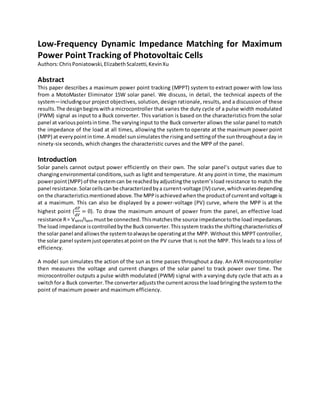
Solar panels cannot output power efficiently on their own. The solar panel’s output varies due to
changingenvironmental conditions,such as light and temperature. At any point in time, the maximum
powerpoint(MPP) of the systemcan be reachedbyadjustingthe system’sload resistance to match the
panel resistance.Solarcellscanbe characterizedbya current-voltage (IV) curve,whichvariesdepending
on the characteristicsmentionedabove.The MPPisachievedwhenthe productof currentand voltage is
at a maximum. This can also be displayed by a power-voltage (PV) curve, where the MPP is at the
highest point (
𝑑𝑃
𝑑𝑉
= 0). To draw the maximum amount of power from the panel, an effective load
resistance R= VMPP/IMPP mustbe connected.Thismatchesthe source impedancetothe loadimpedances.
The load impedance iscontrolledbythe Buckconverter.Thissystem tracksthe shiftingcharacteristicsof
the solar panel andallowsthe systemtoalwaysbe operatingatthe MPP. Without this MPPT controller,
the solar panel systemjustoperatesatpointon the PV curve that is not the MPP. This leads to a loss of
efficiency.
A model sun simulates the action of the sun as time passes throughout a day. An AVR microcontroller
then measures the voltage and current changes of the solar panel to track power over time. The
microcontroller outputs a pulse width modulated (PWM) signal with a varying duty cycle that acts as a
switchfora Buck converter.The converteradjuststhe currentacrossthe loadbringingthe systemtothe
point of maximum power and maximum efficiency.
2. (a) (b)
Figure 1. Solar Panel Characteristics
Methods
MPPT controllers have been created in the past, so the first step that had to be taken for us to create
one was to researchwhatmaincomponentsare typicallyincludedinthe controller. We discovered that
our best option would include a microcontroller, a current monitor, a voltage monitor, and a DC-DC
converter.A model sun,solarpanel,andloadare necessary components to demonstrate the system as
well, but would not be a part of the controller itself. Figure 2 shows how the parts fit together, while
Figure 3 shows a more detailed version of this system block diagram. Once this was determined, the
next step was to look into either acquiring the components or making them ourselves.
Figure 2. System Block Diagram
The solar panel that was used was the MotoMaster Eliminator (15 Watts, 1A), chosen for convenience.
The solar panel was readily available in the adjacent lab and there was a model sun to use with it.
Anotheralternativewasamuch smallersolarpanel, which would not produce enough power to create
the IV graphwe wishedtoproduce.The lastalternative wasthe solarpanel inthe sub-basement of Link
Hall whichhad a model sunalreadyattachedtoit. We did not use this last alternative because it was in
an inconvenient location and there were no added benefits over the first choice.
The DC-DC converter used was a Buck converter. This converter steps down the voltage of the solar
panel to achieve the maximum power. The alternatives are using either a Boost converter or a Buck-
Boostconverter.A Boost converterstepsupthe voltage of the solarpanel andwouldresultininefficient
3. use of solarpoweras well asproduce a voltage toohighforthe load intended for 12V to handle. With a
Boostconverter,the outputvoltage wouldincreaseandthe outputcurrent woulddecrease,resulting in
an inputimpedance greaterthanthe source impedance.Thiswasunacceptable forourpurpose.A Buck-
Boost converter is able to step up and step down the solar panel voltage, but since it is unnecessarily
complicated compared to a simple Buck converter, it was not the best option for our system. A
synchronousBuckconverterwasbuiltfromscratch usingpartsthat were inthe lab or that were ordered
online. A synchronous design was used instead of asynchronous, which involves using two n-channel
MOSFETs instead of one, because it is more efficient. The asynchronous design works by having the
PWM signal control whether a single MOSFET is on or off. When the signal is high, the MOSFET is on;
whenthe signal islow,the MOSFET isoff. This is necessary to control how much the voltage is stepped
down. However it also means that the circuit is disconnected often from the load, whenever the
MOSFET is off. This is the advantage of using the synchronous model. Since it has two MOSFETs, when
one isoff,the other ison and vice versa. This allows the load to always be connected to the rest of the
circuitwhichworksto increase the efficiency of the system. It is not much more difficult to construct a
synchronousBuckconverterinsteadof an asynchronous one, so it was decided that it the synchronous
model would be used in our system design.
Figure 3 belowshowsthe complete circuitschematicincludingthe Buckconverter,the current monitor,
the voltage divider and the microcontroller.
Figure 3. Complete Circuit Schematic
The microcontrollerwasusedtoadjustthe duty cycle of the input signal to the Buck converter in order
to achieve the maximum power. The ATmega328P AVR microcontroller was chosen based on speed,
availability,anddifficultytoprogram. One alternative was an HC12 microcontroller. However, it would
take longerto learnhowto use.Anotheralternative wasusingamicrocontrollerdesigned specificallyfor
MPPT purposes; however this would not be the best option because it was not beneficial enough to
offset the additional complexity of learning to use such a component.
4. To measure voltage andcurrent,the signal intothe ADCport of the microcontroller must be between 0
and 5.5V, and less than 40mA. We used a voltage divider with 1.6kΩ and 5.6kΩ resistors so voltage is
proportionally decreased such that 0V to 22.5V becomes 0V to 5V, or 2/9 of the actual voltage. The
voltage was read by the ADC0 port of the microcontroller. To monitor the current going into the ADC1
port of the microcontroller,anAD8215 currentsensorwas used.A 0.5Ω shunt resistorwasused and the
voltage output of the monitor is calculated by the device as Vout = Iin*10 = Iin*Rshunt*20.
Figure 4. P&O Algorithm Diagram
The Perturband Observe (P&O) algorithmiscommonlyusedinMPPTsystems. It works utilizing a guess
and check method by making small changes to the duty cycle and comparing the new and previous
power values to see which is larger. Based on the previous duty cycle change and the comparison of
powerreadings,the algorithmwill determine whetheritneedstoincrease ordecrease the duty cycle to
get closer to the MPP as shown in Figure 4. See Appendix A-1 for the MPPT microcontroller code.
A lightingsystembuiltbyProfessorDuane Marcy hasbeensetup to model the behavior of the sun. The
Model Sun has thirty-one 54W T5 HO bulbs mounted in an arc and controlled by an MC9S12
microcontroller,whichtreatsthe bulbsasthree sets of eight and one set of seven. It is programmed to
receive four numbers from 0 to 255 via serial communication, where the binary value corresponds to
the orientation of each bank of lights. For example, 11111111 means all the lights of that bank are on,
and 11110000 means only the first four lights are on. Using MATLAB, a program was created to send
valuestothe microcontrollerinordertomimicthe risingandsettingof the sun. The program was set to
take 96 seconds for full cycle to complete, allowing for much faster testing and demonstration than
using the actual sun. In this paper, full sun means each bank was set to 11111111 (binary 255), half sun
corresponds to 10101010 (binary 170) for each bank, and 0001001 (binary 9) was the input for each
bank in the low sun case. See Appendices C-1 and C-2 for the MATLAB code used to control the sun.
Figure 5 below shows the setup of the sun at full sunlight with the solar panel underneath the arc.
5. Figure 5. Model Sun & Solar Panel Setup
The AVR microcontroller was not able to display results or the values of its variables directly to the
computer so indirect methods were used to determine what the values of certain variables were and
how they changed with time. An oscilloscope was used to capture the voltage at the solar panel, the
voltage at the output of the current monitor—which represented the current at the solar panel—and
the PWM signal. In addition to this, the data that the microcontroller read from its ADC ports was
exported to MATLAB via an FTDI board and a UART connection. The receive pin of the FTDI was
connected to the transmit pin of the microcontroller and the FTDI was connected to a laptop via USB.
The USB was registeredin MATLAB as a serial port and the baud rate of that port was set so it matched
that of the microcontrollertransmission.The datawasthenusedtoplotthe power,voltage,currentand
PV curve in real time.See AppendicesB-1andB-2 forthe code used.The values MATLAB received were
not the actual values of the voltage and current, but scaled values of them. Appendix B-3 displays the
MATLAB program usedto determinethe scalingfactorssothe valuesreadincouldbe converted back to
the original data.
At times it was difficult to determine if the system was working correctly or not. A comparison was
needed to verify that the results were correct so data was taken to create the PV curves for full, half,
and low sun. The data was recorded in Excel and scatter plots were made to find which duty cycle was
the correct one to be oscillatingaroundforeachof the three amountsof sunlight.Eachpointisbasedon
the current andvoltage valuesof the solarpanel atdifferent duty cycles in increments of 5% starting at
10% and increasing through 90%. See Figure 6 for the results of those tests.
Basedon the PV curvesobtainedforfull,half,and low sun, a PWMcontroller was designed with a duty
cycle optimizedforhalf sun.45%was an average of the duty cyclesthatcorrespondedto MPPs so it was
chosen as the duty cycle for the PWM controller. The PWMcontroller is an exact replica of the MPPT
controllerexcludingthe changingdutycycle.The P&Oalgorithmwasremovedfromthe microcontroller
6. code for this system and the duty cycle is set to a constant 45%. See Appendix A-2 for the PWM
microcontroller code.
Results
The PV curvesat three levelsof sunlightweremeasuredandplottedwith the results shown in Figure 6.
Figure 6. Experimental PV Curve of Full Sunlight, Half Sunlight, and Low Sunlight
Basedon the resultsfromthe above plots, the peak power value for each level of sunlight was used to
compare to the level of powerateach of those levelsof sunlight using the PWMsystem. The efficiency
of the solar panel was derived from these values and is displayed in the figure below.
Figure 7. Efficiency Comparison
At full and low sun, a 13% and 10% increase in power, respectively, are evident in the MPPT system
comparedto the PWM system.There isnoaddedefficiency in using the MPPT system created over the
PWMsystem created for half sun.
Figures 8, 9, and 10 display the MPPT controller performance. Part (a) of each figure shows the part of
the PV curve that the system is oscillating around. It can be seen that they are oscillating around the
MPP. The blue circle is the most recent data point and the red points are the previous 19 data points.
7. Part (b) of each figure shows the properly scaled, real time power, voltage, and current data being
received from the microcontroller.
(a) (b)
Figure 8. Low Sun, MPPT controller
(a) (b)
Figure 9. Half Sun, MPPT Controller
(a) (b)
Figure 10. Full Sun, MPPT Controller
Figures11, 12, and 13 displaythe PWMcontrollerperformance.Part(a) of eachfigure showsthe part of
the PV curve that the system is operating at. It can be seen that the operating point does not oscillate
and that the power is not necessarily the maxim. The blue circle is the most recent data point and the
red points are the previous 19 data points. Part (b) of each figure shows the properly scaled, real time
power, voltage, and current data being received from the microcontroller.
8. (a) (b)
Figure 11. Low Sun, PWM Controller
(a) (b)
Figure 12. Half Sun, PWM Controller
(a) (b)
Figure 13. Low Sun, PWM Controller
Discussion
It can be seenthatthe maximumpoweris increasingwhenthe amountof sunlight increases for each of
the above situations. For the MPPT system, voltage of the MPP is always around 14V whereas in the
PWMsystemitshiftsall overthe voltage axis. The maximum power of the PWMsystem is shown to be
lowerthan that of the MPPT system though they still increase with respect to amount of sunlight. The
MPPT system never lets the PV curve stray away from that MPP area that is shown in Figure 1(b).
Since the PWMcontrolleroperatesata fixedduty cycle, the optimal PWMcontroller must operate at a
duty cycle that is a statistical average of all the duty cycles that correspond to MPPs across the varying
levelsof sunlight. Thisissothatefficiencyisnot compromised too much for any level of sunlight in the
range that was able to be produced. To create an optimized PWM controller to compare our MPPT
controller to, a duty cycle of 45% was used which is also the duty cycle that corresponds to the MPP of
the systemat half sun.That is whythere isno addedadvantage to using the MPPT controller instead of
the PWM controllerwhenthe sunlight is the equivalent of half sun. As soon as the amount of sunlight
9. drifts from half sun, however, there is an increase in power that the system can draw from the MPPT
controllerwithrespecttothe PWMcontroller.The maximumincrease inpowerdrawnbetweenthe two
controllers occurs at maximum sunlight with an extra 13% efficiency. There is no use to testing the
addedefficiencybelowlowsunlightbecause bothsystemsare the same inthat range.Once the sunlight
drops below a certain point the solar panel does not provide enough energy to power the Buck
converter.Thisessentiallydeactivatesandbypassesthe controller so there will be no difference in the
poweroutputs betweenthe two systems at that input level. Theoretically, based off the data sheet of
the driverusedforthe Buck converter,once the solarpanel voltage dropsbelow 10V the Buck converter
will notwork.However,in practice, we noticed that it was still working until about 9V. Once the panel
voltage drops below that, there will be no efficiency gain between the two controllers.
There are ways to improve our current results. It must be understood that this is still a model system.
While the controllers thatwere builtworkwell,the componentsused to test the system are only rough
models of what would actually be used. The model sun is able to show how the system can track and
adjust when the amount of sunlight changes, but it was not tested outside or in a real time
environment. Also, when the system is deployed it would use a different load than the one that was
used to test the system. A 25Ω power resistor was used which dissipates power whereas a battery, a
more typicallyusedload,wouldhave anearlynegligibleresistance.Itwasnoticedthatasloadresistance
changes,allowedvoltagesfromthe panel change aswell.A lower resistance allows for more current to
flow,andthuslowervoltages,whichallow formore of the full PV curve to existfor the system. This will
not be a problem in terms of finding the MPP because it will still be physically achievable, whereas
shifting to the right can pose a problem in that there is no MPP. A battery was not tested with this
systembecause itwasout of scope for our project, which involved drawing power, not storing it. Also,
the only12V batteryeasilyavailablewasalead-acidbattery.The batteryneeded to be 12V because, for
our solarpanel,thatis where the MPPusually lies. A lead-acid battery, however, is rather complicated
to charge.Simplyapplyinga12.6V will notcharge the batteryproperlyandthere are stagesthat need to
be followed.Itwasdeterminedthattryingtocharge the available batterywouldbe outof scope for this
version of the controller.
The algorithm used for the microcontroller could also be modified to maximize efficiency. The model
sunwas controlledtochange itsamountof lighteverythree seconds. Unless clouds come and go often
and quickly,the sunlightwillnotusuallychange thatquickly.The microcontrollercode couldbe changed
to oscillate less drastically or less often. This would mean that it would sit at the MPP, or closer to it,
longer.One issue with decreasing the duty cycle adjustments to less than 4% is that sometimes that is
too small of a change to notice an accurate change inpower.If there is ever an uncharacteristic jump or
decrease inthe voltage orcurrent,it will give aninaccurate readingforthe power.Thiscouldbe an issue
if,insteadof showingas a decrease in power like it should be, it will show as an increase in power and
therefore willcause the algorithmtomove inthe wrongdirection.Initiallythe dutycycle wasadjustedin
incrementsof 2%but itwas too fine of a scale to give accurate results.Itwasincreasedtoincrements of
4% withsuccessful results.Nothavingthe dutycycle oscillate is out of the question. It is the oscillation
that allows it to notice when the sunlight changes and adjust accordingly. It cannot just find the MPP
and lockontoit. Thisdoes leave some time where the system is actually just slightly off from the MPP
whichisnot optimal forefficiency, but the goal is to have it oscillate fast enough and fine enough that
any variation from the MPP is negligible. For instances where the amount of sunlight changes slowly,
this is an appropriate method. There is always a tradeoff and disadvantage, though. The downside to
having the algorithm adjust often is that the microcontroller uses more power. The disadvantage to
havinga fine dutycycle incrementisthat,if there iseveradrastic change in the amount of sunlight that
the solar panel sees,itwill take longerforthe controllertomove tothe new MPP.A situationwhere this
10. wouldhave a significantimpactishighlyunlikelyorimpossible,though,soitwasnota large factorin the
decision making.
The system that was designed also includes a recalibration technique for the assurance of the correct
MPP beingreached.There were timeswhen the system would get stuck at a certain duty cycle and not
be able to detect any new changes. This was mainly an issue when the lights from the sun were off.
Once the duty cycle got that low,there were manytinyvariationsinpower within a small range of duty
cycles.The algorithm wouldrecognizealocal maximuminsteadof the global maximumandget stuck on
a very low duty cycle even if the lights turned back on and the duty cycle was supposed to increase. A
counterwas addedtothe microcontrollercode sothat every1000 cyclesthe dutycycle will be forced to
reset at 20%. This will allow the system to free itself from any minor local maximums that may be
hinderingthe algorithmfromrecognizingthe actual MPP.Thisdoesnot have a noticeable impact on the
efficiencybecause the microcontrollerisoperatingata fast enoughspeedthatit is able to recover from
the recalibration and move back to the duty cycle corresponding to the MPP extremely quickly. If this
system was being used with the actual sun, this recalibration could be done much less frequently
assuming the light from the sun changes more slowly than the lights from our model sun change.
References
Choudhary,Dhananhay,andAnmol RatnaSaxena.“DC-DCBuck ConverterforMPPTof PV System.”
InternationalJournalof Emerging Technology and Advanced Engineering 4.7(2008): 813-821.
Web.2 March 2016.
Milea,Petru,AdrianZafiu,OrestOltu,andMonicaDascalu.“Theory,AlgorithmsandApplicationsfor
SolarPanel MPP Tracking”. SolarCollectors and Panels,Theory and Applications. Ed.Reccab
Manyala.187-210. Sciyo,2010. Print.
Rosu-Hamzescu,Mihnea,SergiuOprea,andMicrochipTechnologyInc.“Practical Guide toImplementing
SolarPanel MPPT Algorithms.”Microchip.MicrochipTechnology,29November2012. Web.2
March 2016.
11. Appendix A
A-1. MPPT MicrocontrollerCode
/*
* MPPT.cpp
*
* Created: 3/16/2016 12:02:04 PM
* Author : escalzet
*/
#define F_CPU 16000000
#define BAUD 9600
#define BAUD_TOL 3
#include <avr/io.h>
#include <util/setbaud.h>
#include <stdlib.h>
#include <util/delay.h>
#include <avr/common.h>
void initialize_regs();
void start_cycle(int &prev_voltage, long int &prev_pwr, int &updated_voltage, long int
&updated_pwr);
void update_readings(int &prev_voltage, long int &prev_pwr, int &updated_voltage, long
int &updated_pwr);
void read_ADC(int &voltage, int ¤t);
void USART_Init();
void USART_Transmit(unsigned char transData);
int main(void)
{
// declare variables
int updated_voltage, prev_voltage, duty = 50, count = 0;
long int updated_pwr, prev_pwr;
initialize_regs();
start_cycle(prev_voltage, prev_pwr, updated_voltage, updated_pwr); // find
power at 50% and 48% duty cycle
// done initializing
/* Infinite loop to make sure program is always checking */
while (1)
{
// P&O Algorithm
if (updated_pwr > prev_pwr) {
if (updated_voltage > prev_voltage) {
if (duty > 4)
duty -= 4;
}
else {
if (duty < 96)
duty += 4;
}
}
12. else if (updated_pwr < prev_pwr) {
if (updated_voltage > prev_voltage) {
if (duty < 96)
duty += 4;
}
else {
if (duty > 4)
duty -= 4;
}
}
// update duty cycle
if (count != 1000) {
OCR2B = duty;
count++;
}
else {
duty = 20; // allow for recalibration every so often so PWM never
gets stuck in wrong place
OCR2B = duty;
count = 0;
}
_delay_ms(100);
// update power readings
update_readings(prev_voltage, prev_pwr, updated_voltage, updated_pwr);
}
}
void initialize_regs() {
/* initialize registers */
DDRD = 0x08; // D port used to output PWM with correct duty cycle (just need
pin D3 as OC2 output)
// use ADCs for the two inputs
DDRC = 0x00; // need Port C, pins 0 and 1 for inputs
/* initializes ADC registers */
ADMUX |= (1 << REFS0) | (1 << ADLAR); // set reference (max in) to AVcc = 5V
and set ADLAR to 1 - ADLAR left adjusts
// need to set (1 << MUX0) if using ADC1, otherwise (0 << MUX0) if using
ADC0 input
ADCSRA |= (1 << ADEN) | (1 << ADPS2) | (1 << ADPS1); // enables ADC and
prescales to 64 (divides 16MHz by 64 -> input 250kHz clock)
DIDR0 = 0b00111100; // disables pins 2-5 to save power, only allows input from
pins 0/1, pins 6/7 cannot be enabled/disabled but must be 0
/* initializes timer/counter PWM registers */
OCR2A = 99;
OCR2B = 50;
TCCR2A |= (1 << COM2A1) | (1 << COM2B1) | (1 << WGM21) | (1 << WGM20); //
timer/counter control register A chooses fast non-inverted PWM to output at OC2A
13. TCCR2B |= (1 << WGM22) | (1 << CS20); // timer/counter control register B
chooses fast PWM mode, decide not to scale PWM freq since already divided internally
by 256
USART_Init();
}
void start_cycle(int &prev_voltage, long int &prev_pwr, int &updated_voltage, long int
&updated_pwr) {
int current;
/* find power at 50% duty cycle */
read_ADC(prev_voltage, current); // input voltage and current through ADC
prev_pwr = prev_voltage*current;
/* find power at 48% duty cycle */
OCR2B = 48; // update duty
read_ADC(updated_voltage, current); // input voltage and current through ADC
updated_pwr = updated_voltage*current; // I = V / ( Rshunt * 20 )
}
void update_readings(int &prev_voltage, long int &prev_pwr, int &updated_voltage, long
int &updated_pwr) {
int current;
char Txvolt[5] = {' ', ' ', ' ', ' ', ' '}, Txcurr[5]= {' ', ' ', ' ', ' ', '
'};
unsigned char carriage = 'r';
unsigned char newline = 'n';
/* update power readings */
prev_pwr = updated_pwr;
prev_voltage = updated_voltage;
/* input voltage and current through ADC */
read_ADC(updated_voltage, current);
updated_pwr = updated_voltage*current;
/* UART - send voltage and current to MATLAB */
itoa(updated_voltage, Txvolt, 10);
for(int loop = 0; loop < 5; loop++)
USART_Transmit((unsigned char) Txvolt[loop]);
itoa(current, Txcurr, 10);
for(int loop = 0; loop < 5; loop++)
USART_Transmit((unsigned char) Txcurr[loop]);
USART_Transmit(carriage);
USART_Transmit(newline);
14. }
void read_ADC(int &voltage, int ¤t) {
/* input voltage through ADC */
ADMUX = 0b01100000; // set input to ADC0
ADCSRA |= (1 << ADSC); // set ADSC to start conversion
while ( !(ADCSRA & (1 << ADIF) ) ) // Wait until flag is tripped
{
}
ADCSRA |= (1 << ADIF); // Reset flag
voltage = ADCH; // outputs ADC
/* done inputting voltage */
/* input current through ADC */
ADMUX |= (1 << MUX0); // set input to ADC1
ADCSRA |= (1 << ADSC); // set ADSC to start conversion
while ( !(ADCSRA & (1 << ADIF) ) ) // Wait until flag is tripped
{
}
ADCSRA |= (1 << ADIF); // Reset flag
current = ADCH; // outputs ADC
/* done inputting current */
}
void USART_Init(){
DDRD |= (1 << DDD1); // Pin D1 as backup output
UBRR0 = UBRR_VALUE; // Baud rate
if(USE_2X) UCSR0A |= (1 << U2X0); // set double speed if needed
else UCSR0A &= ~(1 << U2X0);
UCSR0B |= (1 << TXEN0); //Tx Enable
UCSR0C |= (1 << UCSZ00)|(1 << UCSZ01); //Falling Edge
}
void USART_Transmit(unsigned char transData){ // sends 1 byte of data over UART
while( !(UCSR0A & (1 << UDRE0)) ); // check status register for any
error flags and that the transmit buffer is clear before writing to transmit buffer
UDR0 = transData; // write the data to the transmit
buffer
}
15. A-2. PWMMicrocontrollerCode
/*
* PWM.cpp
*
* Created: 4/22/2016 6:28:54 PM
* Author : Computer
*/
#define F_CPU 16000000
#define BAUD 9600
#define BAUD_TOL 3
#include <avr/io.h>
#include <util/setbaud.h>
#include <stdlib.h>
#include <util/delay.h>
#include <avr/common.h>
void initialize_regs();
void update_readings(int &prev_voltage, long int &prev_pwr, int &updated_voltage, long
int &updated_pwr);
void read_ADC(int &voltage, int ¤t);
void USART_Init();
void USART_Transmit(unsigned char transData);
int main(void)
{
// declare variables
int updated_voltage, prev_voltage;
long int updated_pwr, prev_pwr;
initialize_regs();
/* Infinite loop to make sure program is always checking */
while (1)
{
// update power readings
update_readings(prev_voltage, prev_pwr, updated_voltage, updated_pwr);
}
}
void initialize_regs() {
/* initialize registers */
DDRD = 0x08; // D port used to output PWM with correct duty cycle (just need
pin D3 as OC2 output)
// use ADCs for the two inputs
DDRC = 0x00; // need Port C, pins 0 and 1 for inputs
/* initializes ADC registers */
ADMUX |= (1 << REFS0) | (1 << ADLAR); // set reference (max in) to AVcc = 5V
and set ADLAR to 1 - ADLAR left adjusts
// need to set (1 << MUX0) if using ADC1, otherwise (0 << MUX0) if using ADC0
input
16. ADCSRA |= (1 << ADEN) | (1 << ADPS2) | (1 << ADPS1); // enables ADC and
prescales to 64 (divides 16MHz by 64 -> input 250kHz clock)
DIDR0 = 0b00111100; // disables pins 2-5 to save power, only allows input from
pins 0/1, pins 6/7 cannot be enabled/disabled but must be 0
/* initializes timer/counter PWM registers */
OCR2A = 99;
OCR2B = 44;
TCCR2A |= (1 << COM2A1) | (1 << COM2B1) | (1 << WGM21) | (1 << WGM20); //
timer/counter control register A chooses fast non-inverted PWM to output at OC2A
TCCR2B |= (1 << WGM22) | (1 << CS20); // timer/counter control register B
chooses fast PWM mode, decide not to scale PWM freq since already divided internally
by 256
USART_Init();
}
void update_readings(int &prev_voltage, long int &prev_pwr, int &updated_voltage, long
int &updated_pwr) {
int current;
char Txvolt[5] = {' ', ' ', ' ', ' ', ' '}, Txcurr[5]= {' ', ' ', ' ', ' ', '
'};
unsigned char carriage = 'r';
unsigned char newline = 'n';
/* update power readings */
prev_pwr = updated_pwr;
prev_voltage = updated_voltage;
/* input voltage and current through ADC */
read_ADC(updated_voltage, current);
updated_pwr = updated_voltage*current;
/* UART - send voltage and current to MATLAB */
itoa(updated_voltage, Txvolt, 10);
for(int loop = 0; loop < 5; loop++)
USART_Transmit((unsigned char) Txvolt[loop]);
itoa(current, Txcurr, 10);
for(int loop = 0; loop < 5; loop++)
USART_Transmit((unsigned char) Txcurr[loop]);
USART_Transmit(carriage);
USART_Transmit(newline);
}
void read_ADC(int &voltage, int ¤t) {
/* input voltage through ADC */
ADMUX = 0b01100000; // set input to ADC0
ADCSRA |= (1 << ADSC); // set ADSC to start conversion
17. while ( !(ADCSRA & (1 << ADIF) ) ) // Wait until flag is tripped
{
}
ADCSRA |= (1 << ADIF); // Reset flag
voltage = ADCH; // outputs ADC
/* done inputting voltage */
/* input current through ADC */
ADMUX |= (1 << MUX0); // set input to ADC1
ADCSRA |= (1 << ADSC); // set ADSC to start conversion
while ( !(ADCSRA & (1 << ADIF) ) ) // Wait until flag is tripped
{
}
ADCSRA |= (1 << ADIF); // Reset flag
current = ADCH; // outputs ADC
/* done inputting current */
}
void USART_Init(){
DDRD |= (1 << DDD1); // Pin D1 as backup output
UBRR0 = UBRR_VALUE; // Baud rate
if(USE_2X) UCSR0A |= (1 << U2X0); // set double speed if needed
else UCSR0A &= ~(1 << U2X0);
UCSR0B |= (1 << TXEN0); //Tx Enable
UCSR0C |= (1 << UCSZ00)|(1 << UCSZ01); //Falling Edge
}
void USART_Transmit(unsigned char transData){ // sends 1 byte of data over UART
while( !(UCSR0A & (1 << UDRE0)) ); // check status register for any
error flags and that the transmit buffer is clear before writing to transmit buffer
UDR0 = transData; // write the data to the transmit
buffer
}
19. xlim(ax3,[t(i)-4 t(i)+1])
drawnow
%pause(.1);
t(i+1)=t(i)+toc;
end
B-2. Display PV Curve in MATLAB in Real Time
m.ReadAsyncMode = 'manual';
pts = 2000;
len = 20;
j = 1;
pwr=nan([1,len]);
vlt=nan([1,len]);
figure;
%whitebg('black');
pv=scatter(NaN,NaN,'r');
grid on;
title('PV Characteristic');
ylabel('Power [W]'); xlabel('Voltage [V]');
axis([0 20 0 4]);
hold;
newpv=scatter(NaN,NaN,'b');
for i=1:pts
stuff=0; %make numel(stuff)~=2
while numel(stuff)~=2 || stuff(1)>274 || stuff(2)>571 %(max 25V 2A) %updated
4/21/16 5:16PM
stuff = str2num(fgets(m));
end
vlt(j)=stuff(1)/10.9861; cur(j)=stuff(2)/0.4893; %updated 4/21/16 10:00PM
pwr(j) = vlt(j)*cur(j)/1000;
set(pv,'XData',vlt,'YData',pwr)
set(newpv,'XData',vlt(j),'YData',pwr(j))
drawnow
if j == len
j = 1;
else
j = j+1;
end
end
20. B-3. Find ScalingFactors for MATLAB
m.ReadAsyncMode = 'manual';
pts=20;
vlt=nan([1,pts]);
cur=nan([1,pts]);
stuff=0;
for i=1:pts
stuff=0; %make numel(stuff)~=2
while numel(stuff)~=2 || stuff(1)>274 || stuff(2)>571 %(max 25V 2A) %updated
4/21/16 5:16PM
stuff = str2num(fgets(m));
end
vlt(i)=stuff(1)/10.9861; cur(i)=stuff(2)/0.4893; %updated 4/21/16 10:00PM
end
mean(vlt)
mean(cur)
21. Appendix C
C-1. Set Each Light in Model Sun
function [ ] = setlights(s, bank)
%SETLIGHTS Configures lighting of sun to desired on/off values
% sends 's' character followed by four numbers (0-255)
% specified by matrix BANK, and ends with sending the LF
% (Line Feed) control character (ASCII Code 10)
% to serial port associated with serial port object s.
fwrite(s,'s');
fwrite(s,bank(1));
fwrite(s,bank(2));
fwrite(s,bank(3));
fwrite(s,bank(4));
fprintf(s,'');
end
C-2. Have Lights IncrementallyTurn On/Off
%% NOTE: BANK(2)=128 DOES NOT EXIST
%% (8th light of bank 2 or top/center light)
delay=3; % make sure delay>1 to give bulb enough time to turn on
%Connect to serial port
%s = serial('COM3', 'BaudRate', 9600);
%fopen(s);
%initialize each bank as off
bank = [0 0 0 0];
setlights(s,bank);
pause(1);
%double lights moving back and forth: (ctrl+C to stop execution)
while 1
%forward
for i = 1:4
for j=0:2:6 %0 2 4 6
bank(i)=bank(i)+2^j+2^(j+1);
setlights(s,bank);
pause(delay);
end
end
%backward
for i = 4:-1:1
for j=6:-2:0 %6 4 2 0
bank(i)=bank(i)-2^j-2^(j+1);
setlights(s,bank);
pause(delay);
end
end
end