Measures of variability are used to quantify how spread out or dispersed a data set is from the average. There are several common measures, including range, quartile deviation, standard deviation, variance, and coefficient of variation. Range is the simplest measure and finds the difference between the highest and lowest values. Quartile deviation examines the middle 50% of data. Standard deviation finds the average distance from the mean and is the most stable measure. Variance squares the standard deviation. Coefficient of variation allows comparison of variability between variables with different units.

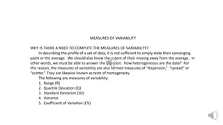
1. MEASURES OF VARIABILITY
WHY IS THERE A NEED TO COMPUTE THE MEASURES OF VARIABILITY?
In describing the profile of a set of data, it is not sufficient to simply state their converging
point or the average. We should also know the extent of their moving away from the average. In
other words, we must be able to answer the question: How heterogeneous are the data? For
this reason, the measures of variability are also termed measures of “dispersion,” “spread” or
“scatter.” They are likewise known as tests of homogeneity.
The following are measures of variability:
1. Range (R)
2. Quartile Deviation (Q)
3. Standard Deviation (SD)
4. Variance
5. Coefficient of Variation (CV)

2. RANGE
RANGE is the difference between the highest score/value and the lowest score/value
Plus 1. This measure of variability is resorted to when one wishes to get a quick and rough
estimate of the variability of a set of values/scores. The formula for RANGE is:
R = (Highest Score/Value – Lowest Score/Value) + 1
QUARTILE DEVIATION
The Quartile Deviation (Q) is otherwise known as Semi-Interquartile Range. It is one-half of
the range between the third quartile (Q3) and the first quartile (Q1). This measure is used to
determine the density of the middle 50 % of the distribution. Its formula is as follows:
Q = Q3 -- Q1
2

3. Where Q is the computed quartile deviation
Q3 = L + .75N - < Fi
f
Q1 = L + .25N - < Fi
f
And where L = the lower limit of the Q3 or Q1 class
N = the total number of cases
<F = cumulative frequency BEFORE the Q3 and Q1 class
f = original frequency of the Q3 or Q1 class
I = size of the class interval
Q3 class = the class interval containing .75N
Q1 class = the class interval containing .25N
STEPS IN COMPUTING FOR Q
1. Solve for Q3
a. Construct the <F column.
b. Determine .75N and locate this under the <F column. Draw a line to enclose
the class interval containing the .75N. Mark this as Q3 class.
c. Obtain the following: L, <F, f, i, N.
d. Substitute the values in the formula. Compute for Q3.

4. 2. Solve for Q1
a. Construct the < F column.
b. Determine .25N and locate this under the <F column. Draw a line to enclose the class
interval containing the .25N. Mark this as Q1 class.
c. Obtain the following : L, <F, f, i, N.
d. Substitute the values in the formula. Compute for Q1.
3. Solve for Q by substituting Q3 and Q1 in the formula,
Q = Q3 -- Q1
2

5. Sample Computation of Q
Given the following score distribution, determine the quartile deviation.
c. i. f <F
195 – 199 1 50
I = 5 190 – 194 2 49
185 – 189 4 47
180 – 184 5 43
L (for Q3) 175 – 179 8 f (for Q3) 38 Q3 class
---174.5 170 – 174 10 30 <F (for Q3)
165 – 169 6 20
L (for Q1) 160 – 164 4 f (for Q1) 14 Q1 class
---- 159.5 155 – 159 4 10 <F (for Q1)
150 – 154 2 6
145 – 149 3 4
140 – 144 1 1

6. Solution:
a. Q3
.75N = .75 (50) = 37.5 Locate this under <F (contained in 38 with c.i. 175 – 179)
LQ3 = 174.5, <F = 30, f = 8, i = 5, N = 50
Q3 = L + ( .75N -- <F) i
( f )
Q3 = 174.5 + ( 37.5 – 30 ) 5
( 8 )
= 174.5 + ( 7.5 ) 5
8
= 174.5 + (.94)5
= 174.5 + 4.7
= 179.2
b. Q1
.25N = .25(50) = 12.5 Locate this under <F (contained in 14 with c.i. 160-164)
LQ1 = 159.5, <F = 10, f = 4, i = 5, N = 50
Q1 = L + ( .25N -- <F) I
f

7. Q1 = 159.5 + (12.5 – 10)5
( 4 )
= 159.5 + ( 2. 5)5
( 4 )
= 159.5 + (.63)5
= 159.5 + 3.15
= 162.65
c. Solve for Q
Q = Q3 -- Q1
2
= 179.2 - 162.65
2
= 16.55
2
Q = 8.28

8. STANDARD DEVIATION
The Standard Deviation (SD) is the root-mean-square of deviations of the individual scores
around the mean. It is the MOST STABLE MEASURE OF VARIABILITY. It can be computed for a set of
ungrouped data (<30 cases) or for grouped data (> 30 cases or more grouped into a frequency
distribution.)
Standard Deviation for Ungrouped Data
For a set of data less than 30 cases, standard deviation can be computed by using the formula
Ʃ(Xi -- X)2
N - 1
σ =
where σ =standard deviation
Ʃ = sum of
Xi = individual scores/values
X = mean of the individual scores/values
N = total number of cases (scores/values)

9. Sample computation for SD (ungrouped data)
Example: Given the following set of scores, compute for the σ.
XI : 25, 20, 22, 26, 23, 25, 27, 20, 28, 30
Solution:
Xi ( Xi - X) (Xi - X)2
25 .4 .16
20 -4.6 21.16
22 -2.6 6.76
26 1.4 1.96
23 -1.6 2.56
25 .4 .16
27 2.4 5.76
20 -4.6 21.16
28 3.4 11.56
30 5.4 29.16
Steps: 246/10=24.6 Ʃ(Xi –X)2 = 100.40
1. Compute for the Mean. (X=24.6)
2. Subtract the mean from each of the given values. (Xi – X)
3. Square each of the values obtained in Step2, then get the sum of the squared values.
4. Substitute the values in the formula and compute for the σ

13. VARIANCE
Variance is simply the square of the standard deviation. Thus, its formula is
2
V = (SD)
COEFFICIENT OF VARIATION
This measure indicates the variation of a group in two different variables. It may be
computed under the following conditions:
a. When the units of measurement are incommensurable (not similar)
b. When the means are not equal.
The formula for the coefficient of variation is:
CV = SD x 100
M
where CV = the computed coefficient of variation
SD = standard deviation
M = mean

14. Example:
The heights and weights of 40 Grade Six pupils were taken and the following data were
obtained after some computation:
Height (H) Weight(W)
MH = 4.8’ MW = 96 lbs.
SDH = .6 SDW = 5.4 ibs
Question: In which trait is the group more variable.?
Solution:
a) CV for Height b) CV for Weight
CV = SD x 100 CV = SD x 100
M M
= .6 X 100 = 5.4 X 100
4.8 96
= .125 X 100 = .05625 X 100
CV = 12.5% CV = 5.63%
Answer: The group is more variable in terms of height.