Image filtering

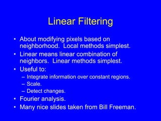
1. Linear Filtering
• About modifying pixels based on
neighborhood. Local methods simplest.
• Linear means linear combination of
neighbors. Linear methods simplest.
• Useful to:
– Integrate information over constant regions.
– Scale.
– Detect changes.
• Fourier analysis.
• Many nice slides taken from Bill Freeman.

2. (Freeman)

3. (Freeman)

4. Correlation
Examples on white board – 1D
Examples -2D

5. For example, let’s take a vector like:
(1 2 3 2 3 2 1), and filter it with a filter like (1/3 1/3 1/3)
Ignoring the ends for the moment, we get a result like:
2 2 1/3 2 2/3 2 1/3 2. We can also graph the results
and see that the original vector is smoothed out.

6. Boundaries
• Zeros
• Repeat values
• Cycle
• Produce shorter result
• Examples

7. Correlation





N
N
i
i
x
I
i
F
x
I
F )
(
)
(
)
(

 

 




N
N
j
N
N
i
j
y
i
x
I
j
i
F
y
x
I
F )
,
(
)
,
(
)
,
(

For this notation, we index F from –N to N.

8. Convolution
• Like Correlation with Filter Reversed
• Associative






N
N
i
i
x
I
i
F
x
I
F )
(
)
(
)
(
 

 





N
N
j
N
N
i
j
y
i
x
I
j
i
F
y
x
I
F )
,
(
)
,
(
)
,
(
1D
2D

9. Some Examples

24. Filtering to reduce noise
• Noise is what we’re not interested in.
– We’ll discuss simple, low-level noise today:
Light fluctuations; Sensor noise;
Quantization effects; Finite precision
– Not complex: shadows; extraneous
objects.
• A pixel’s neighborhood contains
information about its intensity.
• Averaging noise reduces its effect.

25. Additive noise
• I = S + N. Noise doesn’t depend on
signal.
• We’ll consider:
d
distribute
y
identicall
,
for
t
independen
,
tic.
determinis
0
)
(
with
j
i
j
i
j
i
i
i
i
i
i
n
n
n
n
n
n
s
n
E
n
s
I





26. Average Filter
• Mask with positive
entries, that sum 1.
• Replaces each pixel
with an average of
its neighborhood.
• If all weights are
equal, it is called a
BOX filter.
1
1
1
1
1 1
1
1
1
F
1/9
(Camps)

27. Averaging Filter and noise
reduction
• Example: try executing:
k=1; figure(1); hist(sum((1/k)*rand(k,1000)))
for different values of k.
• The average of noise is smaller than one example.
– This is intuitive
– Can be proven in many cases (some technical conditions:
noise must be independent, many samples….)
– Actually true for many real examples: Gaussian noise,
flipping a coin many times

28. Filtering reduces noise if signal
stable
• Suppose I(i) = I+n(i), I(i+1) = I+n(i+1)
I(i+2) = I+n(i+2).
• Average of I(i), I(i+1), I(i+2) = I +
average of n(i), n(i+1), n(i+2).
• When there is no noise, averaging
smooths the signal.
• So in real life, averaging does both.

29. Example: Smoothing by
Averaging

30. Smoothing as Inference About
the Signal
+ =
Nearby points tell more about the
signal than distant ones.
Neighborhood for
averaging.

31. Gaussian Averaging
• Rotationally
symmetric.
• Weights nearby
pixels more than
distant ones.
– This makes sense
as probabalistic
inference.
• A Gaussian gives a
good model of a fuzzy
blob

32. An Isotropic Gaussian
• The picture shows a
smoothing kernel
proportional to
(which is a reasonable
model of a circularly
symmetric fuzzy
blob)
  




 

 2
2
2
0
2
exp
2
1
)
,
(



y
x
y
x
G

33. Smoothing with a Gaussian

34. The effects of smoothing
Each row shows smoothing
with gaussians of different
width; each column shows
different realizations of
an image of gaussian noise.

35. Efficient Implementation
• Both, the BOX filter and the Gaussian
filter are separable:
– First convolve each row with a 1D filter
– Then convolve each column with a 1D
filter.

36. Box Filter











































0
0
0
3
1
3
1
3
1
0
0
0
0
3
1
0
0
3
1
0
0
3
1
0
9
1
9
1
9
1
9
1
9
1
9
1
9
1
9
1
9
1


37. Gaussian Filter
    












 

 2
2
2
2
2
2
2
0
2
exp
2
exp
2
1
2
exp
2
1
)
,
(







y
x
y
x
y
x
G

38. Smoothing as Inference About
the Signal: Non-linear Filters.
+ =
What’s the best
neighborhood for
inference?

39. Filtering to reduce noise:
Lessons
• Noise reduction is probabilistic
inference.
• Depends on knowledge of signal and
noise.
• In practice, simplicity and efficiency
important.

40. Filtering and Signal
• Smoothing also smooths signal.
• Matlab
• Removes detail
• Matlab
• This is good and bad:
- Bad: can’t remove noise w/out blurring
shape.
- Good: captures large scale structure;
allows subsampling.

41. Subsampling
Matlab