SlideShare a Scribd company logo
1 of 19
Download to read offline
ECE4510/5510: Feedback Control Systems. 5–1
STABILITY ANALYSIS
5.1: Bounded-input bounded-output (BIBO) stability
I A system may be “stable,” “neutrally or marginally stable,” or
“unstable.” This can be illustrated using cones:
Stable Neutral Unstable
• The cone in the “stable” configuration can be perturbed by nudging
it from any direction, and its position will not change much.
• The cone in the “neutral” configuration can be nudged in the axial
direction without changing its position much, but if it is nudged in
the radial direction, it will roll and its position will change a lot. (The
“stability” of a neutral system depends on the input.)
• The cone in the “unstable” position can be nudged from any
direction, and its position will change a lot.
I We want stability because we don’t want a small input (e.g., possibly
disturbance, or a small change in the reference input) to cause the
output to grow without bound (seem to become “uncontrolled”).
I In system analysis, there are many ways to mathematically define
and evaluate whether a system is stable.
Lecture notes prepared by and copyright c 1998–2013, Gregory L. Plett and M. Scott Trimboli
ECE4510/ECE5510, STABILITY ANALYSIS 5–2
I For LTI systems, all are basically the same, and equivalent to
“bounded-input bounded-output” or BIBO stability.
I If the system’s input is bounded by some positive constant K1
|u(t)| < K1 ∀t
then BIBO stability guarantees that the output will also be bounded by
some (possibly different) positive constant K2
|y(t)| < K2 ∀t.
I In the time domain,
y(t) =
∞
−∞
h(τ)u(t − τ) dτ
|y(t)| =
∞
−∞
h(τ)u(t − τ) dτ
≤
∞
−∞
|h(τ)| |u(t − τ)| dτ
≤ K1
∞
−∞
|h(τ)| dτ.
I So, |y(t)| < ∞ iff
∞
−∞
|h(τ)| dτ < ∞. This is one test for BIBO
stability.
y(t)u(t) C Stable? Note: (h(t) = 1(t)).
I Integrating the absolute value of a function can be very tricky.
Sometimes it’s easier to integrate a simpler function that gives an
upper bound instead.
I Consider h(t) = exp(−t) sin(2πt)1(t). Is this system BIBO stable?
Lecture notes prepared by and copyright c 1998–2013, Gregory L. Plett and M. Scott Trimboli
ECE4510/ECE5510, STABILITY ANALYSIS 5–3
I The blue line in the figure is h(t);
and the green dotted line is |h(t)|.
I To determine stability, we need to
integrate to find the area under the
green dotted line—if this area is
finite, then the system is stable.
h(t)
|h(t)|
exp(−t)
I Finding the exact answer for this integral is hard. But, the integral
under the green dotted line is less than the integral under the red line.
I So, if the integral under the red line is finite, the system is stable.
∞
0
e−t
dt = −e−t ∞
0
= 1.
I So, we have determined that the system is BIBO stable, and we
didn’t need to integrate a very challenging piecewise function.
I We can also evaluate BIBO stability in the Laplace domain:
H(s) =
Y(s)
R(s)
=
K m
1 (s − zi)
n
1(s − pi)
m ≤ n.
(assume poles unique)
h(t) =
n
i=1
kiepi t
1(t)
∞
−∞
|h(τ)| dτ < ∞ iff R(pi) < 0 ∀ i.
(If poles are not distinct, h(t) will have terms
k
(m − 1)!
tm−1
epi t
for an mth order root.
Lecture notes prepared by and copyright c 1998–2013, Gregory L. Plett and M. Scott Trimboli
ECE4510/ECE5510, STABILITY ANALYSIS 5–4
∞
−∞
|h(τ)| dτ < ∞ iff R(pi) < 0;
Same condition.)
I Laplace-domain condition for stability: All poles in the transfer
function must be in the open left hand plane. (i.e., none on jω axis.)
EXAMPLE: T(s) =
2
s2 + 3s + 2
. Is T(s) stable?
T (s) =
2
(s + 1)(s + 2)
,
I Roots at s = −1, s = −2. Stable!
EXAMPLE: T(s) =
10s + 24
s3 + 2s2 − 11s − 12
. Is T (s) stable?
T (s) =
10(s + 2.4)
(s + 1)(s − 3)(s + 4)
,
I Roots at s = −1, s = +3, s = −4. Unstable!
EXAMPLE: T(s) =
s
s2 + 1
. Is T (s) stable?
T(s) =
s
(s − j)(s + j)
,
I Roots at s = ± j. MARGINALLY stable.
I Use input = sin(t).
Y(s) =
s
s2 + 1
1
s2 + 1
=
s
(s2 + 1)2
y(t) =
1
2
t sin(t) . . . unbounded.
I MARGINALLY stable = unstable (bounded impulse response, but
unbounded output for some inputs.)
Lecture notes prepared by and copyright c 1998–2013, Gregory L. Plett and M. Scott Trimboli
ECE4510/ECE5510, STABILITY ANALYSIS 5–5
5.2: Routh–Hurwitz stability (cases 0 and 1)
I Factoring high-degree polynomials to find roots is tedious and
numerically not well conditioned.
I Want other stability tests, and also MARGINS of stability.
(1) Routh test
(2) Root locus
(3) Nyquist test
(4) Bode stability margins



Can you tell this is
an important topic?
I In 1868, Maxwell found conditions on the coefficients of a transfer
function polynomial of 2nd and 3rd order to guarantee stability.
I It became the subject of the 1877 Adams Prize to determine
conditions for stability for higher-order polynomials.
I Routh won this prize, and the method is still useful.
Routh test “case 0”
I Consider the denominator a(s).
2nd order:
a(s) = s2
+ a1s + a0 = (s − p1)(s − p2) = s2
− (p1 + p2)s + p1 p2.
3rd order:
a(s) = s3
+ a2s2
+ a1s + a0
= (s − p1)(s − p2)(s − p3)
= s2
− (p1 + p2)s + p1 p2 s − p3
Lecture notes prepared by and copyright c 1998–2013, Gregory L. Plett and M. Scott Trimboli
ECE4510/ECE5510, STABILITY ANALYSIS 5–6
= s3
− (p1 + p2 + p3)s2
+ (p1 p2 + p1 p3 + p2 p3)s − p1 p2 p3.
TREND: Stability « none of the coefficients ai can be ≤ 0.
Does this trend continue?
an−1 = (−1)× sum of all roots.
an−2 = sum of products of roots taken two at a time.
an−3 = (−1)× sum of products of roots taken three at a time.
...
a0 = (−1)n
× product of all roots.
I Conclusions:
1. If any coefficient ai = 0, not all roots in LHP.
2. If any coefficient ai < 0, at least one root in RHP.
TEST: If any coefficient ai ≤ 0, system is unstable.
EXAMPLE: a(s) = s2
+ 0s + 1.
I From conclusion (1), not all roots in LHP.
I Roots at s = ± j.
I “Marginally” stable.
EXAMPLE: a(s) = s3
+ 2s2
− 11s − 12.
I From conclusion (2), at least one root is in RHP.
I Roots at s = −1, s = −4, s = +3.
I Unstable.
EXAMPLE: a(s) = s3
+ s2
+ 2s + 8.
Lecture notes prepared by and copyright c 1998–2013, Gregory L. Plett and M. Scott Trimboli
ECE4510/ECE5510, STABILITY ANALYSIS 5–7
I We don’t know yet if this system is stable or not.
I Roots at s = −2, s =
1
2
±
j
√
15
2
. Unstable, but how do we find out
without factoring?
Routh test “case 1”
I Once we have determined that ai > 0 ∀ i, we need to run the full
Routh test (“case 0” doesn’t really count).
I Very mechanical, not intuitive. Proof difficult.
I Start with characteristic polynomial (denominator of closed-loop
transfer function), a(s) = sn
+ an−1sn−1
+ · · · + a1s + a0.
I Form “Routh array”.
• First two rows are coefficients directly copied from a(s);
• Remaining rows are calculated as shown.
sn
an an−2 an−4 · · ·
sn−1
an−1 an−3 an−5 · · ·
sn−2
b1 b2 · · ·
sn−3
c1 c2 · · ·
...
s1
j1
s0
k1
b1 =
−1
an−1
an an−2
an−1 an−3
b2 =
−1
an−1
an an−4
an−1 an−5
· · ·
c1 =
−1
b1
an−1 an−3
b1 b2
c2 =
−1
b1
an−1 an−5
b1 b3
· · ·
TEST: Number of unstable roots = number of sign changes in left column.
Lecture notes prepared by and copyright c 1998–2013, Gregory L. Plett and M. Scott Trimboli
ECE4510/ECE5510, STABILITY ANALYSIS 5–8
EXAMPLE: a(s) = s3
+ s2
+ 2s + 8.
s3
1 2
s2
1 8
s1
−6
s0
8 b1 =
−1
1
1 2
1 8
= −(8 − 2) = −6
c1 =
−1
−6
1 8
−6 0
=
1
6
(0 + 6 × 8) = 8
I Two sign changes (1 → −6, −6 → 8) Two roots in RHP.
EXAMPLE: a(s) = s2
+ a1s + a0.
s2
1 a0
s1
a1
s0
a0
b1 =
−1
a1
1 a0
a1 0
=
−1
a1
(0 − a0a1) = a0
I Stable iff a1 > 0, a0 > 0.
EXAMPLE: a(s) = s3
+ a2s2
+ a1s + a0.
s3
1 a1
s2
a2 a0
s1
a1 −
a0
a2
s0
a0
b1 =
−1
a2
1 a1
a2 a0
=
−1
a2
(a0 − a1a2)
= a1 −
a0
a2
c1 =
−1
b1
a2 a0
b1 0
=
−1
b1
(−a0b1) = a0.
I Stable iff a2 > 0, a0 > 0, a1 >
a0
a2
.
Lecture notes prepared by and copyright c 1998–2013, Gregory L. Plett and M. Scott Trimboli
ECE4510/ECE5510, STABILITY ANALYSIS 5–9
5.3: Routh–Hurwitz stability (cases 2 and 3)
Routh test “case 2”
I In the process of filling in the Routh array, we sometimes find an
element in first column = 0.
I This leads to a divide by zero computation in a subsequent step,
which has an indeterminate result.
I Solution: Replace the zero in the left column with ± as → 0. (Will
get same result for + and − .)
EXAMPLE: a(s) = s5
+ 2s4
+ 2s3
+ 4s2
+ 11s + 10.
s5
1 2 11
s4
2 4 10
s3
0 6
new s3
6
s2 −12
10
s1
6
s0
10
If > 0, two sign changes.
If < 0, two sign changes.
« Two poles in RHP.
b1 =
−1
2
1 2
2 4
=
−1
2
(4 − 4) = 0
b2 =
−1
2
1 11
2 10
=
−1
2
(10 − 22) = 6
c1 =
−1 2 4
6
=
−1
(12 − 4 ) ≈
−12
c2 =
−1 2 10
0
=
−1
(0 − 10 ) = 10
d1 =
12
6
−12
10
=
12
(10 +
72
) ≈ 6
e1 =
−1
6
−12
10
6 0
=
−1
6
(0 − 60) = 10
Lecture notes prepared by and copyright c 1998–2013, Gregory L. Plett and M. Scott Trimboli
ECE4510/ECE5510, STABILITY ANALYSIS 5–10
Routh test “case 3”
I Sometimes an entire row in Routh array = 0.
I This means that polynomial factors such that one factor has
conjugate-MIRROR-roots, which can be configured as shown in the
figure:
I(s)
R(s)
I(s)
R(s)
I(s)
R(s)
I In any case, system is unstable. But how many RHP roots?
I Complete Routh array by making polynomial a1(s) from last non-zero
row in array. Poly has every second order of s only!!
• We do this in a reverse fashion from how we entered a(s) into the
array in the first place.
I It turns out that a1(s) is a factor of the original a(s). It is missing some
orders of s, so IS NOT STABLE (by “case 0”.)
I We want to see if it has roots in the RHP or only on the jω-axis.
I Replace zero row with coefficients from
da1(s)
ds
and continue.
Lecture notes prepared by and copyright c 1998–2013, Gregory L. Plett and M. Scott Trimboli
ECE4510/ECE5510, STABILITY ANALYSIS 5–11
EXAMPLE: a(s) = s4
+ s3
+ 3s2
+ 2s + 2.
s4
1 3 2
s3
1 2 0
s2
1 2
s1
0
new s1
2
s0
2
No sign changes in Routh
array. So, no RHP roots.
Roots of a1(s) at s = ± j
√
2.
Marginally stable.
b1 =
−1
1
1 3
1 2
= 1
b2 =
−1
1
1 2
1 0
= 2
c1 =
−1
1
1 2
1 2
= 0
a1(s) = s2
+ 2
da1(s)
ds
= 2s
d1 =
−1
2
1 2
2 0
= 2
EXAMPLE: a(s) = s4
+ 4 (Hard).
s4
1 0 4
s3
0 0
new s3
4 0
s2
0 4
new s2
4
s1 −16
s0
4
Two sign changes. Therefore
2 RHP poles. Other two
poles are mirrors in LHP.
a1(s) = s4
+ 4;
da1(s)
ds
= 4s3
.
b1 =
−1
4
1 0
4 0
= 0
b2 =
−1
4
1 4
4 0
= 4
c1 =
−1 4 0
4
=
−16
d1 =
16
4
−16
0
= 4
Lecture notes prepared by and copyright c 1998–2013, Gregory L. Plett and M. Scott Trimboli
ECE4510/ECE5510, STABILITY ANALYSIS 5–12
5.4: Routh test as a design tool
I Consider the system:
R(s) Y(s)K
s + 1
s(s − 1)(s + 6)
T(s) =
Y(s)
R(s)
=
K s+1
s(s−1)(s+6)
1 + K s+1
s(s−1)(s+6)
=
K(s + 1)
s(s − 1)(s + 6) + K(s + 1)
I We might be interested in knowing for what values of K the system is
stable.
I Compute the denominator of the transfer function:
a(s) = s(s − 1)(s + 6) + K(s + 1)
= s3
+ 5s2
+ (K − 6)s + K.
I Perform the Routh test
s3
1 K − 6
s2
5 K
s1 4K − 30
5
s0
K
b1 =
−1
5
1 K − 6
5 K
=
−1
5
(K − 5(K − 6))
= (4K − 30)/5.
c1 =
−1
b1
5 K
b1 0
=
−1
b1
(−b1K) = K
I For stability of the closed-loop system, K > 0, and K > 30/4.
I Step response for different values of K.
Lecture notes prepared by and copyright c 1998–2013, Gregory L. Plett and M. Scott Trimboli
ECE4510/ECE5510, STABILITY ANALYSIS 5–13
0 2 4 6 8 10 12
−0.5
0
0.5
1
1.5
2
2.5
K=7.5
K=13
K=25
Amplitude
Time (sec.)
EXAMPLE:
R(s) Y(s)K 1 +
1
TI s
1
(s + 1)(s + 2)
T (s) =
Y(s)
R(s)
=
K TI s+K
TI s(s+1)(s+2)
1 + K TI s+K
TI s(s+1)(s+2)
=
K TI s + K
TI s(s + 1)(s + 2) + K TI s + K
.
I a(s) = TI s3
+ 3TI s2
+ TI (2 + K)s + K.
s3
TI TI (2 + K)
s2
3TI K
s1
TI (K + 2) −
K
3
s0
K
b1 =
−1
3TI
TI TI (2 + K)
3TI K
= TI (K + 2) −
K
3
c1 =
−1
b1
3TI K
b1 0
=
−1
b1
(−b1K) = K
Lecture notes prepared by and copyright c 1998–2013, Gregory L. Plett and M. Scott Trimboli
ECE4510/ECE5510, STABILITY ANALYSIS 5–14
I For stability of the closed-loop system, K > 0 and TI > 0 and
TI >
K
3(K + 2)
.
I Alternately, K < 0 and TI < 0 and TI <
K
3(K + 2)
for −2 < K < 0, (or
instead TI >
K
3(K + 2)
for K < −2 but this is a contradiction since the
quotient is positive and TI is negative by assumption).
0 2 4 6 8 10 12
0
0.5
1
1.5
Time (seconds)
K = 3, TI = 0.5
K = 1, TI = 0.25
K = 1, TI = ∞
Amplitude
Lecture notes prepared by and copyright c 1998–2013, Gregory L. Plett and M. Scott Trimboli
ECE4510/ECE5510, STABILITY ANALYSIS 5–15
5.5: Advanced applications of the Routh test
I Note that the Routh test is not specifically a controls recipe.
• It is a geometric algorithm.
• It counts the number of roots of a polynomial that have R(si) ≥ 0.
Modification #1
I Suppose we want to ensure a settling-time specification (or some
form of robust stability), so we want R(si) ≤ −σ for all poles.
I Routh test doesn’t apply directly; but, perform a change of variables:
• Let p = s + σ. Then, si < −σ corresponds to pi < 0.
I So, we can perform a Routh test on a(p) instead of a(s).
EXAMPLE: Let T (s) =
K
s2 + 4s + K
. For what values of K are all poles to
the left of s = −1?
I Note, σ = 1, and we let p = s + 1 or s = p − 1.
T (p) =
K
(p − 1)2 + 4(p − 1) + K
=
K
p2 − 2p + 1 + 4p − 4 + K
=
K
p2 + 2p + K − 3
.
I So, a(p) = p2
+ 2p + (K − 3). Form the Routh array:
p2
1 (K − 3)
p1
2
p0
(K − 3)
I If K > 3, the real part of all poles of
T(s) are less than −1. −5 −4 −3 −2 −1 0 1
−2
−1.5
−1
−0.5
0
0.5
1
1.5
2
Real axis
Imaginaryaxis
Root locus
K = 3
Lecture notes prepared by and copyright c 1998–2013, Gregory L. Plett and M. Scott Trimboli
ECE4510/ECE5510, STABILITY ANALYSIS 5–16
Modification #2
I When working with digital control systems, the complex frequency
domain is represented by “z” instead of “s”, and a system is stable if
all poles of T (z) have magnitude strictly less than 1.
I The stability region is the unit circle in
the z-plane.
I The Routh test does not apply directly.
I But, we can perform the change of variables (where α > 0)
z =
1 + αs
1 − αs
or s =
1
α
z − 1
z + 1
,
which is known as the bilinear transformation.
I We can show that this transformation maps the inside of the unit
circle in the z-plane to the left-half s-plane.
I Let z = rejθ
. We have stability if z < 1. So, we want to show that r < 1
produces R(s) < 0.
I Substituting into the change of variables
s =
1
α
rejθ
− 1
rejθ + 1
=
1
α
rejθ
− 1
rejθ + 1
re− jθ
+ 1
re− jθ + 1
=
1
α





r2
− 1 +
j2r sin θ
rejθ
− re− jθ
r2 + 1 + rejθ
+ re− jθ
2r cos θ





.
I Note that:
Lecture notes prepared by and copyright c 1998–2013, Gregory L. Plett and M. Scott Trimboli
ECE4510/ECE5510, STABILITY ANALYSIS 5–17
• When r = 1, s is purely imaginary (translating the unit circle into
the jω axis)
• When r < 1, the real part of s is less than zero (translating the
inside of the unit disc into the left-half s-plane)
• When r > 1, the real part of s is greater than zero (translating the
outside of the unit disc into the right-half s-plane).
EXAMPLE: Let T (z) =
K
z + (K − 0.5)
.
I We can see from inspection (for this simple example) that
−0.5 < K < 1.5 will result in a pole location that is between z = −1
and z = +1.
I But, let’s perform the bilinear transformation and the Routh test.
Choose α = 1.
T (s) = T (z)|z=1+s
1−s
=
K
1+s
1−s
+ (K − 0.5)
=
K(1 − s)
1 + s + (K − 0.5)(1 − s)
=
K(1 − s)
(1.5 − K)s + (K + 0.5)
.
I Form the (trivial) Routh array:
s1
(1.5 − K)
s0
(K + 0.5)
I So, we have stability when K < 1.5 and
when K > −0.5, as expected.
Lecture notes prepared by and copyright c 1998–2013, Gregory L. Plett and M. Scott Trimboli
ECE4510/ECE5510, STABILITY ANALYSIS 5–18
5.6: Internal stability
I BIBO stability requires that the output be bounded for every possible
bounded input.
I However, a system may be input-output stable and still have
unbounded internal signals.
I The issue is internal stability.
I Consider the following diagram:
R(s)
E(s) U(s)
W(s)
Y(s)D(s) G(s)
I We can find the following four transfer functions:
Y(s)
R(s)
=
D(s)G(s)
1 + D(s)G(s)
Y(s)
W(s)
=
G(s)
1 + D(s)G(s)
.
U(s)
R(s)
=
D(s)
1 + D(s)G(s)
U(s)
W(s)
=
1
1 + D(s)G(s)
.
I For internal stability, all four of these transfer functions must be stable.
EXAMPLE: Let G(s) =
1
s − 1
and D(s) =
s − 1
s + 1
.
I Then,
Y(s)
R(s)
=
D(s)G(s)
1 + D(s)G(s)
=
s−1
(s−1)(s+1)
1 + s−1
(s−1)(s+1)
Lecture notes prepared by and copyright c 1998–2013, Gregory L. Plett and M. Scott Trimboli
ECE4510/ECE5510, STABILITY ANALYSIS 5–19
=
s − 1
(s − 1)(s + 1) + (s − 1)
=
1
s + 1 + 1
=
1
s + 2
.
I This system passes the test for BIBO stability.
I However,
Y(s)
W(s)
=
G(s)
1 + D(s)G(s)
=
1
s−1
1 + s−1
(s−1)(s+1)
=
s + 1
(s − 1)(s + 1) + (s − 1)
=
s + 1
(s − 1)(s + 2)
,
which is unstable.
I Therefore, this system is not internally stable.
I In this case, any (even very tiny) amount of disturbance will cause the
output y(t) to grow without bound. The feedback will not help.
I This brings up the point that it is important to avoid “bad”
cancellations of pole-zero pairs!
I We cannot stabilize a system by canceling an unstable pole with a
compensator zero.
• We will see the same idea again from a different perspective when
we look at root-locus design.
Lecture notes prepared by and copyright c 1998–2013, Gregory L. Plett and M. Scott Trimboli

More Related Content

What's hot

Lecture 6 modelling-of_electrical__electronic_systems
Lecture 6 modelling-of_electrical__electronic_systemsLecture 6 modelling-of_electrical__electronic_systems
Lecture 6 modelling-of_electrical__electronic_systemsSaifullah Memon
 
Modern Control - Lec 02 - Mathematical Modeling of Systems
Modern Control - Lec 02 - Mathematical Modeling of SystemsModern Control - Lec 02 - Mathematical Modeling of Systems
Modern Control - Lec 02 - Mathematical Modeling of SystemsAmr E. Mohamed
 
Controllability and observability
Controllability and observabilityControllability and observability
Controllability and observabilityjawaharramaya
 
Lecture 2 transfer-function
Lecture 2 transfer-functionLecture 2 transfer-function
Lecture 2 transfer-functionSaifullah Memon
 
State space analysis shortcut rules, control systems,
State space analysis shortcut rules, control systems, State space analysis shortcut rules, control systems,
State space analysis shortcut rules, control systems, Prajakta Pardeshi
 
Current commutated chopper
Current commutated chopperCurrent commutated chopper
Current commutated chopperJyoti Singh
 
Frequency Response Analysis
Frequency Response AnalysisFrequency Response Analysis
Frequency Response AnalysisHussain K
 
Lecture 4 ME 176 2 Mathematical Modeling
Lecture 4 ME 176 2 Mathematical ModelingLecture 4 ME 176 2 Mathematical Modeling
Lecture 4 ME 176 2 Mathematical ModelingLeonides De Ocampo
 
Control system lectures
Control system lectures Control system lectures
Control system lectures Naqqash Sajid
 
State space analysis, eign values and eign vectors
State space analysis, eign values and eign vectorsState space analysis, eign values and eign vectors
State space analysis, eign values and eign vectorsShilpa Shukla
 
Laplace transform and its applications
Laplace transform and its applicationsLaplace transform and its applications
Laplace transform and its applicationsNisarg Shah
 
Laplace Transformation & Its Application
Laplace Transformation & Its ApplicationLaplace Transformation & Its Application
Laplace Transformation & Its ApplicationChandra Kundu
 
NONLINEAR CONTROL SYSTEM (Phase plane & Phase Trajectory Method)
NONLINEAR CONTROL SYSTEM(Phase plane & Phase Trajectory Method)NONLINEAR CONTROL SYSTEM(Phase plane & Phase Trajectory Method)
NONLINEAR CONTROL SYSTEM (Phase plane & Phase Trajectory Method)Niraj Solanki
 

What's hot (20)

Lecture 6 modelling-of_electrical__electronic_systems
Lecture 6 modelling-of_electrical__electronic_systemsLecture 6 modelling-of_electrical__electronic_systems
Lecture 6 modelling-of_electrical__electronic_systems
 
Modern Control - Lec 02 - Mathematical Modeling of Systems
Modern Control - Lec 02 - Mathematical Modeling of SystemsModern Control - Lec 02 - Mathematical Modeling of Systems
Modern Control - Lec 02 - Mathematical Modeling of Systems
 
Stability ppt
Stability pptStability ppt
Stability ppt
 
Controllability and observability
Controllability and observabilityControllability and observability
Controllability and observability
 
Lecture 2 transfer-function
Lecture 2 transfer-functionLecture 2 transfer-function
Lecture 2 transfer-function
 
State space analysis shortcut rules, control systems,
State space analysis shortcut rules, control systems, State space analysis shortcut rules, control systems,
State space analysis shortcut rules, control systems,
 
Current commutated chopper
Current commutated chopperCurrent commutated chopper
Current commutated chopper
 
Frequency Response Analysis
Frequency Response AnalysisFrequency Response Analysis
Frequency Response Analysis
 
Lecture 23 24-time_response
Lecture 23 24-time_responseLecture 23 24-time_response
Lecture 23 24-time_response
 
Lecture 4 ME 176 2 Mathematical Modeling
Lecture 4 ME 176 2 Mathematical ModelingLecture 4 ME 176 2 Mathematical Modeling
Lecture 4 ME 176 2 Mathematical Modeling
 
Signal flow graph
Signal flow graphSignal flow graph
Signal flow graph
 
Control system lectures
Control system lectures Control system lectures
Control system lectures
 
State space analysis, eign values and eign vectors
State space analysis, eign values and eign vectorsState space analysis, eign values and eign vectors
State space analysis, eign values and eign vectors
 
Laplace transform and its applications
Laplace transform and its applicationsLaplace transform and its applications
Laplace transform and its applications
 
system properties
system propertiessystem properties
system properties
 
Transient analysis
Transient analysisTransient analysis
Transient analysis
 
Laplace Transformation & Its Application
Laplace Transformation & Its ApplicationLaplace Transformation & Its Application
Laplace Transformation & Its Application
 
NONLINEAR CONTROL SYSTEM (Phase plane & Phase Trajectory Method)
NONLINEAR CONTROL SYSTEM(Phase plane & Phase Trajectory Method)NONLINEAR CONTROL SYSTEM(Phase plane & Phase Trajectory Method)
NONLINEAR CONTROL SYSTEM (Phase plane & Phase Trajectory Method)
 
6. steady state error
6. steady state error6. steady state error
6. steady state error
 
Lecture 4: Classification of system
Lecture 4: Classification of system Lecture 4: Classification of system
Lecture 4: Classification of system
 

Similar to Control Systems - Stability Analysis.

K11038 Mayur control ppt
K11038 Mayur control pptK11038 Mayur control ppt
K11038 Mayur control pptChetan Kumar
 
Stabiltiy & R-H Ccriterion
Stabiltiy & R-H CcriterionStabiltiy & R-H Ccriterion
Stabiltiy & R-H CcriterionHussain K
 
lecture 10 formal methods in software enginnering.pptx
lecture 10 formal methods in software enginnering.pptxlecture 10 formal methods in software enginnering.pptx
lecture 10 formal methods in software enginnering.pptxSohaibAlviWebster
 
CSE680-07QuickSort.pptx
CSE680-07QuickSort.pptxCSE680-07QuickSort.pptx
CSE680-07QuickSort.pptxDeepakM509554
 
Circuit Network Analysis - [Chapter5] Transfer function, frequency response, ...
Circuit Network Analysis - [Chapter5] Transfer function, frequency response, ...Circuit Network Analysis - [Chapter5] Transfer function, frequency response, ...
Circuit Network Analysis - [Chapter5] Transfer function, frequency response, ...Simen Li
 
EC8352-Signals and Systems - Laplace transform
EC8352-Signals and Systems - Laplace transformEC8352-Signals and Systems - Laplace transform
EC8352-Signals and Systems - Laplace transformNimithaSoman
 
Control and Instrumentation.pdf.pdf
Control and Instrumentation.pdf.pdfControl and Instrumentation.pdf.pdf
Control and Instrumentation.pdf.pdfMahamad Jawhar
 
Skiena algorithm 2007 lecture09 linear sorting
Skiena algorithm 2007 lecture09 linear sortingSkiena algorithm 2007 lecture09 linear sorting
Skiena algorithm 2007 lecture09 linear sortingzukun
 
Approximate Bayesian Computation with Quasi-Likelihoods
Approximate Bayesian Computation with Quasi-LikelihoodsApproximate Bayesian Computation with Quasi-Likelihoods
Approximate Bayesian Computation with Quasi-LikelihoodsStefano Cabras
 
Redundancy in robot manipulators and multi robot systems
Redundancy in robot manipulators and multi robot systemsRedundancy in robot manipulators and multi robot systems
Redundancy in robot manipulators and multi robot systemsSpringer
 

Similar to Control Systems - Stability Analysis. (20)

Ece4510 notes06
Ece4510 notes06Ece4510 notes06
Ece4510 notes06
 
Ece4510 notes07
Ece4510 notes07Ece4510 notes07
Ece4510 notes07
 
K11038 Mayur control ppt
K11038 Mayur control pptK11038 Mayur control ppt
K11038 Mayur control ppt
 
Routh
RouthRouth
Routh
 
Stabiltiy & R-H Ccriterion
Stabiltiy & R-H CcriterionStabiltiy & R-H Ccriterion
Stabiltiy & R-H Ccriterion
 
lecture 10 formal methods in software enginnering.pptx
lecture 10 formal methods in software enginnering.pptxlecture 10 formal methods in software enginnering.pptx
lecture 10 formal methods in software enginnering.pptx
 
CSE680-07QuickSort.pptx
CSE680-07QuickSort.pptxCSE680-07QuickSort.pptx
CSE680-07QuickSort.pptx
 
Ece4510 notes08
Ece4510 notes08Ece4510 notes08
Ece4510 notes08
 
Circuit Network Analysis - [Chapter5] Transfer function, frequency response, ...
Circuit Network Analysis - [Chapter5] Transfer function, frequency response, ...Circuit Network Analysis - [Chapter5] Transfer function, frequency response, ...
Circuit Network Analysis - [Chapter5] Transfer function, frequency response, ...
 
EC8352-Signals and Systems - Laplace transform
EC8352-Signals and Systems - Laplace transformEC8352-Signals and Systems - Laplace transform
EC8352-Signals and Systems - Laplace transform
 
CLIM Fall 2017 Course: Statistics for Climate Research, Nonstationary Covaria...
CLIM Fall 2017 Course: Statistics for Climate Research, Nonstationary Covaria...CLIM Fall 2017 Course: Statistics for Climate Research, Nonstationary Covaria...
CLIM Fall 2017 Course: Statistics for Climate Research, Nonstationary Covaria...
 
Ch06 6
Ch06 6Ch06 6
Ch06 6
 
Ece4510 notes04
Ece4510 notes04Ece4510 notes04
Ece4510 notes04
 
Control and Instrumentation.pdf.pdf
Control and Instrumentation.pdf.pdfControl and Instrumentation.pdf.pdf
Control and Instrumentation.pdf.pdf
 
Skiena algorithm 2007 lecture09 linear sorting
Skiena algorithm 2007 lecture09 linear sortingSkiena algorithm 2007 lecture09 linear sorting
Skiena algorithm 2007 lecture09 linear sorting
 
Approximate Bayesian Computation with Quasi-Likelihoods
Approximate Bayesian Computation with Quasi-LikelihoodsApproximate Bayesian Computation with Quasi-Likelihoods
Approximate Bayesian Computation with Quasi-Likelihoods
 
Ece4510 notes03
Ece4510 notes03Ece4510 notes03
Ece4510 notes03
 
Signals and Systems Assignment Help
Signals and Systems Assignment HelpSignals and Systems Assignment Help
Signals and Systems Assignment Help
 
TLT
TLTTLT
TLT
 
Redundancy in robot manipulators and multi robot systems
Redundancy in robot manipulators and multi robot systemsRedundancy in robot manipulators and multi robot systems
Redundancy in robot manipulators and multi robot systems
 

Recently uploaded

Call Girls Service Nagpur Tanvi Call 7001035870 Meet With Nagpur Escorts
Call Girls Service Nagpur Tanvi Call 7001035870 Meet With Nagpur EscortsCall Girls Service Nagpur Tanvi Call 7001035870 Meet With Nagpur Escorts
Call Girls Service Nagpur Tanvi Call 7001035870 Meet With Nagpur EscortsCall Girls in Nagpur High Profile
 
The Most Attractive Pune Call Girls Budhwar Peth 8250192130 Will You Miss Thi...
The Most Attractive Pune Call Girls Budhwar Peth 8250192130 Will You Miss Thi...The Most Attractive Pune Call Girls Budhwar Peth 8250192130 Will You Miss Thi...
The Most Attractive Pune Call Girls Budhwar Peth 8250192130 Will You Miss Thi...ranjana rawat
 
Call Girls in Nagpur Suman Call 7001035870 Meet With Nagpur Escorts
Call Girls in Nagpur Suman Call 7001035870 Meet With Nagpur EscortsCall Girls in Nagpur Suman Call 7001035870 Meet With Nagpur Escorts
Call Girls in Nagpur Suman Call 7001035870 Meet With Nagpur EscortsCall Girls in Nagpur High Profile
 
Call Girls Pimpri Chinchwad Call Me 7737669865 Budget Friendly No Advance Boo...
Call Girls Pimpri Chinchwad Call Me 7737669865 Budget Friendly No Advance Boo...Call Girls Pimpri Chinchwad Call Me 7737669865 Budget Friendly No Advance Boo...
Call Girls Pimpri Chinchwad Call Me 7737669865 Budget Friendly No Advance Boo...roncy bisnoi
 
Java Programming :Event Handling(Types of Events)
Java Programming :Event Handling(Types of Events)Java Programming :Event Handling(Types of Events)
Java Programming :Event Handling(Types of Events)simmis5
 
Call for Papers - Educational Administration: Theory and Practice, E-ISSN: 21...
Call for Papers - Educational Administration: Theory and Practice, E-ISSN: 21...Call for Papers - Educational Administration: Theory and Practice, E-ISSN: 21...
Call for Papers - Educational Administration: Theory and Practice, E-ISSN: 21...Christo Ananth
 
(SHREYA) Chakan Call Girls Just Call 7001035870 [ Cash on Delivery ] Pune Esc...
(SHREYA) Chakan Call Girls Just Call 7001035870 [ Cash on Delivery ] Pune Esc...(SHREYA) Chakan Call Girls Just Call 7001035870 [ Cash on Delivery ] Pune Esc...
(SHREYA) Chakan Call Girls Just Call 7001035870 [ Cash on Delivery ] Pune Esc...ranjana rawat
 
Extrusion Processes and Their Limitations
Extrusion Processes and Their LimitationsExtrusion Processes and Their Limitations
Extrusion Processes and Their Limitations120cr0395
 
MANUFACTURING PROCESS-II UNIT-5 NC MACHINE TOOLS
MANUFACTURING PROCESS-II UNIT-5 NC MACHINE TOOLSMANUFACTURING PROCESS-II UNIT-5 NC MACHINE TOOLS
MANUFACTURING PROCESS-II UNIT-5 NC MACHINE TOOLSSIVASHANKAR N
 
Microscopic Analysis of Ceramic Materials.pptx
Microscopic Analysis of Ceramic Materials.pptxMicroscopic Analysis of Ceramic Materials.pptx
Microscopic Analysis of Ceramic Materials.pptxpurnimasatapathy1234
 
(MEERA) Dapodi Call Girls Just Call 7001035870 [ Cash on Delivery ] Pune Escorts
(MEERA) Dapodi Call Girls Just Call 7001035870 [ Cash on Delivery ] Pune Escorts(MEERA) Dapodi Call Girls Just Call 7001035870 [ Cash on Delivery ] Pune Escorts
(MEERA) Dapodi Call Girls Just Call 7001035870 [ Cash on Delivery ] Pune Escortsranjana rawat
 
(ANVI) Koregaon Park Call Girls Just Call 7001035870 [ Cash on Delivery ] Pun...
(ANVI) Koregaon Park Call Girls Just Call 7001035870 [ Cash on Delivery ] Pun...(ANVI) Koregaon Park Call Girls Just Call 7001035870 [ Cash on Delivery ] Pun...
(ANVI) Koregaon Park Call Girls Just Call 7001035870 [ Cash on Delivery ] Pun...ranjana rawat
 
OSVC_Meta-Data based Simulation Automation to overcome Verification Challenge...
OSVC_Meta-Data based Simulation Automation to overcome Verification Challenge...OSVC_Meta-Data based Simulation Automation to overcome Verification Challenge...
OSVC_Meta-Data based Simulation Automation to overcome Verification Challenge...Soham Mondal
 
Sheet Pile Wall Design and Construction: A Practical Guide for Civil Engineer...
Sheet Pile Wall Design and Construction: A Practical Guide for Civil Engineer...Sheet Pile Wall Design and Construction: A Practical Guide for Civil Engineer...
Sheet Pile Wall Design and Construction: A Practical Guide for Civil Engineer...Dr.Costas Sachpazis
 
VIP Call Girls Service Hitech City Hyderabad Call +91-8250192130
VIP Call Girls Service Hitech City Hyderabad Call +91-8250192130VIP Call Girls Service Hitech City Hyderabad Call +91-8250192130
VIP Call Girls Service Hitech City Hyderabad Call +91-8250192130Suhani Kapoor
 
The Most Attractive Pune Call Girls Manchar 8250192130 Will You Miss This Cha...
The Most Attractive Pune Call Girls Manchar 8250192130 Will You Miss This Cha...The Most Attractive Pune Call Girls Manchar 8250192130 Will You Miss This Cha...
The Most Attractive Pune Call Girls Manchar 8250192130 Will You Miss This Cha...ranjana rawat
 
College Call Girls Nashik Nehal 7001305949 Independent Escort Service Nashik
College Call Girls Nashik Nehal 7001305949 Independent Escort Service NashikCollege Call Girls Nashik Nehal 7001305949 Independent Escort Service Nashik
College Call Girls Nashik Nehal 7001305949 Independent Escort Service NashikCall Girls in Nagpur High Profile
 
(RIA) Call Girls Bhosari ( 7001035870 ) HI-Fi Pune Escorts Service
(RIA) Call Girls Bhosari ( 7001035870 ) HI-Fi Pune Escorts Service(RIA) Call Girls Bhosari ( 7001035870 ) HI-Fi Pune Escorts Service
(RIA) Call Girls Bhosari ( 7001035870 ) HI-Fi Pune Escorts Serviceranjana rawat
 
Structural Analysis and Design of Foundations: A Comprehensive Handbook for S...
Structural Analysis and Design of Foundations: A Comprehensive Handbook for S...Structural Analysis and Design of Foundations: A Comprehensive Handbook for S...
Structural Analysis and Design of Foundations: A Comprehensive Handbook for S...Dr.Costas Sachpazis
 
Processing & Properties of Floor and Wall Tiles.pptx
Processing & Properties of Floor and Wall Tiles.pptxProcessing & Properties of Floor and Wall Tiles.pptx
Processing & Properties of Floor and Wall Tiles.pptxpranjaldaimarysona
 

Recently uploaded (20)

Call Girls Service Nagpur Tanvi Call 7001035870 Meet With Nagpur Escorts
Call Girls Service Nagpur Tanvi Call 7001035870 Meet With Nagpur EscortsCall Girls Service Nagpur Tanvi Call 7001035870 Meet With Nagpur Escorts
Call Girls Service Nagpur Tanvi Call 7001035870 Meet With Nagpur Escorts
 
The Most Attractive Pune Call Girls Budhwar Peth 8250192130 Will You Miss Thi...
The Most Attractive Pune Call Girls Budhwar Peth 8250192130 Will You Miss Thi...The Most Attractive Pune Call Girls Budhwar Peth 8250192130 Will You Miss Thi...
The Most Attractive Pune Call Girls Budhwar Peth 8250192130 Will You Miss Thi...
 
Call Girls in Nagpur Suman Call 7001035870 Meet With Nagpur Escorts
Call Girls in Nagpur Suman Call 7001035870 Meet With Nagpur EscortsCall Girls in Nagpur Suman Call 7001035870 Meet With Nagpur Escorts
Call Girls in Nagpur Suman Call 7001035870 Meet With Nagpur Escorts
 
Call Girls Pimpri Chinchwad Call Me 7737669865 Budget Friendly No Advance Boo...
Call Girls Pimpri Chinchwad Call Me 7737669865 Budget Friendly No Advance Boo...Call Girls Pimpri Chinchwad Call Me 7737669865 Budget Friendly No Advance Boo...
Call Girls Pimpri Chinchwad Call Me 7737669865 Budget Friendly No Advance Boo...
 
Java Programming :Event Handling(Types of Events)
Java Programming :Event Handling(Types of Events)Java Programming :Event Handling(Types of Events)
Java Programming :Event Handling(Types of Events)
 
Call for Papers - Educational Administration: Theory and Practice, E-ISSN: 21...
Call for Papers - Educational Administration: Theory and Practice, E-ISSN: 21...Call for Papers - Educational Administration: Theory and Practice, E-ISSN: 21...
Call for Papers - Educational Administration: Theory and Practice, E-ISSN: 21...
 
(SHREYA) Chakan Call Girls Just Call 7001035870 [ Cash on Delivery ] Pune Esc...
(SHREYA) Chakan Call Girls Just Call 7001035870 [ Cash on Delivery ] Pune Esc...(SHREYA) Chakan Call Girls Just Call 7001035870 [ Cash on Delivery ] Pune Esc...
(SHREYA) Chakan Call Girls Just Call 7001035870 [ Cash on Delivery ] Pune Esc...
 
Extrusion Processes and Their Limitations
Extrusion Processes and Their LimitationsExtrusion Processes and Their Limitations
Extrusion Processes and Their Limitations
 
MANUFACTURING PROCESS-II UNIT-5 NC MACHINE TOOLS
MANUFACTURING PROCESS-II UNIT-5 NC MACHINE TOOLSMANUFACTURING PROCESS-II UNIT-5 NC MACHINE TOOLS
MANUFACTURING PROCESS-II UNIT-5 NC MACHINE TOOLS
 
Microscopic Analysis of Ceramic Materials.pptx
Microscopic Analysis of Ceramic Materials.pptxMicroscopic Analysis of Ceramic Materials.pptx
Microscopic Analysis of Ceramic Materials.pptx
 
(MEERA) Dapodi Call Girls Just Call 7001035870 [ Cash on Delivery ] Pune Escorts
(MEERA) Dapodi Call Girls Just Call 7001035870 [ Cash on Delivery ] Pune Escorts(MEERA) Dapodi Call Girls Just Call 7001035870 [ Cash on Delivery ] Pune Escorts
(MEERA) Dapodi Call Girls Just Call 7001035870 [ Cash on Delivery ] Pune Escorts
 
(ANVI) Koregaon Park Call Girls Just Call 7001035870 [ Cash on Delivery ] Pun...
(ANVI) Koregaon Park Call Girls Just Call 7001035870 [ Cash on Delivery ] Pun...(ANVI) Koregaon Park Call Girls Just Call 7001035870 [ Cash on Delivery ] Pun...
(ANVI) Koregaon Park Call Girls Just Call 7001035870 [ Cash on Delivery ] Pun...
 
OSVC_Meta-Data based Simulation Automation to overcome Verification Challenge...
OSVC_Meta-Data based Simulation Automation to overcome Verification Challenge...OSVC_Meta-Data based Simulation Automation to overcome Verification Challenge...
OSVC_Meta-Data based Simulation Automation to overcome Verification Challenge...
 
Sheet Pile Wall Design and Construction: A Practical Guide for Civil Engineer...
Sheet Pile Wall Design and Construction: A Practical Guide for Civil Engineer...Sheet Pile Wall Design and Construction: A Practical Guide for Civil Engineer...
Sheet Pile Wall Design and Construction: A Practical Guide for Civil Engineer...
 
VIP Call Girls Service Hitech City Hyderabad Call +91-8250192130
VIP Call Girls Service Hitech City Hyderabad Call +91-8250192130VIP Call Girls Service Hitech City Hyderabad Call +91-8250192130
VIP Call Girls Service Hitech City Hyderabad Call +91-8250192130
 
The Most Attractive Pune Call Girls Manchar 8250192130 Will You Miss This Cha...
The Most Attractive Pune Call Girls Manchar 8250192130 Will You Miss This Cha...The Most Attractive Pune Call Girls Manchar 8250192130 Will You Miss This Cha...
The Most Attractive Pune Call Girls Manchar 8250192130 Will You Miss This Cha...
 
College Call Girls Nashik Nehal 7001305949 Independent Escort Service Nashik
College Call Girls Nashik Nehal 7001305949 Independent Escort Service NashikCollege Call Girls Nashik Nehal 7001305949 Independent Escort Service Nashik
College Call Girls Nashik Nehal 7001305949 Independent Escort Service Nashik
 
(RIA) Call Girls Bhosari ( 7001035870 ) HI-Fi Pune Escorts Service
(RIA) Call Girls Bhosari ( 7001035870 ) HI-Fi Pune Escorts Service(RIA) Call Girls Bhosari ( 7001035870 ) HI-Fi Pune Escorts Service
(RIA) Call Girls Bhosari ( 7001035870 ) HI-Fi Pune Escorts Service
 
Structural Analysis and Design of Foundations: A Comprehensive Handbook for S...
Structural Analysis and Design of Foundations: A Comprehensive Handbook for S...Structural Analysis and Design of Foundations: A Comprehensive Handbook for S...
Structural Analysis and Design of Foundations: A Comprehensive Handbook for S...
 
Processing & Properties of Floor and Wall Tiles.pptx
Processing & Properties of Floor and Wall Tiles.pptxProcessing & Properties of Floor and Wall Tiles.pptx
Processing & Properties of Floor and Wall Tiles.pptx
 

Control Systems - Stability Analysis.

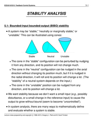
  • 1. ECE4510/5510: Feedback Control Systems. 5–1 STABILITY ANALYSIS 5.1: Bounded-input bounded-output (BIBO) stability I A system may be “stable,” “neutrally or marginally stable,” or “unstable.” This can be illustrated using cones: Stable Neutral Unstable • The cone in the “stable” configuration can be perturbed by nudging it from any direction, and its position will not change much. • The cone in the “neutral” configuration can be nudged in the axial direction without changing its position much, but if it is nudged in the radial direction, it will roll and its position will change a lot. (The “stability” of a neutral system depends on the input.) • The cone in the “unstable” position can be nudged from any direction, and its position will change a lot. I We want stability because we don’t want a small input (e.g., possibly disturbance, or a small change in the reference input) to cause the output to grow without bound (seem to become “uncontrolled”). I In system analysis, there are many ways to mathematically define and evaluate whether a system is stable. Lecture notes prepared by and copyright c 1998–2013, Gregory L. Plett and M. Scott Trimboli
  • 2. ECE4510/ECE5510, STABILITY ANALYSIS 5–2 I For LTI systems, all are basically the same, and equivalent to “bounded-input bounded-output” or BIBO stability. I If the system’s input is bounded by some positive constant K1 |u(t)| < K1 ∀t then BIBO stability guarantees that the output will also be bounded by some (possibly different) positive constant K2 |y(t)| < K2 ∀t. I In the time domain, y(t) = ∞ −∞ h(τ)u(t − τ) dτ |y(t)| = ∞ −∞ h(τ)u(t − τ) dτ ≤ ∞ −∞ |h(τ)| |u(t − τ)| dτ ≤ K1 ∞ −∞ |h(τ)| dτ. I So, |y(t)| < ∞ iff ∞ −∞ |h(τ)| dτ < ∞. This is one test for BIBO stability. y(t)u(t) C Stable? Note: (h(t) = 1(t)). I Integrating the absolute value of a function can be very tricky. Sometimes it’s easier to integrate a simpler function that gives an upper bound instead. I Consider h(t) = exp(−t) sin(2πt)1(t). Is this system BIBO stable? Lecture notes prepared by and copyright c 1998–2013, Gregory L. Plett and M. Scott Trimboli
  • 3. ECE4510/ECE5510, STABILITY ANALYSIS 5–3 I The blue line in the figure is h(t); and the green dotted line is |h(t)|. I To determine stability, we need to integrate to find the area under the green dotted line—if this area is finite, then the system is stable. h(t) |h(t)| exp(−t) I Finding the exact answer for this integral is hard. But, the integral under the green dotted line is less than the integral under the red line. I So, if the integral under the red line is finite, the system is stable. ∞ 0 e−t dt = −e−t ∞ 0 = 1. I So, we have determined that the system is BIBO stable, and we didn’t need to integrate a very challenging piecewise function. I We can also evaluate BIBO stability in the Laplace domain: H(s) = Y(s) R(s) = K m 1 (s − zi) n 1(s − pi) m ≤ n. (assume poles unique) h(t) = n i=1 kiepi t 1(t) ∞ −∞ |h(τ)| dτ < ∞ iff R(pi) < 0 ∀ i. (If poles are not distinct, h(t) will have terms k (m − 1)! tm−1 epi t for an mth order root. Lecture notes prepared by and copyright c 1998–2013, Gregory L. Plett and M. Scott Trimboli
  • 4. ECE4510/ECE5510, STABILITY ANALYSIS 5–4 ∞ −∞ |h(τ)| dτ < ∞ iff R(pi) < 0; Same condition.) I Laplace-domain condition for stability: All poles in the transfer function must be in the open left hand plane. (i.e., none on jω axis.) EXAMPLE: T(s) = 2 s2 + 3s + 2 . Is T(s) stable? T (s) = 2 (s + 1)(s + 2) , I Roots at s = −1, s = −2. Stable! EXAMPLE: T(s) = 10s + 24 s3 + 2s2 − 11s − 12 . Is T (s) stable? T (s) = 10(s + 2.4) (s + 1)(s − 3)(s + 4) , I Roots at s = −1, s = +3, s = −4. Unstable! EXAMPLE: T(s) = s s2 + 1 . Is T (s) stable? T(s) = s (s − j)(s + j) , I Roots at s = ± j. MARGINALLY stable. I Use input = sin(t). Y(s) = s s2 + 1 1 s2 + 1 = s (s2 + 1)2 y(t) = 1 2 t sin(t) . . . unbounded. I MARGINALLY stable = unstable (bounded impulse response, but unbounded output for some inputs.) Lecture notes prepared by and copyright c 1998–2013, Gregory L. Plett and M. Scott Trimboli
  • 5. ECE4510/ECE5510, STABILITY ANALYSIS 5–5 5.2: Routh–Hurwitz stability (cases 0 and 1) I Factoring high-degree polynomials to find roots is tedious and numerically not well conditioned. I Want other stability tests, and also MARGINS of stability. (1) Routh test (2) Root locus (3) Nyquist test (4) Bode stability margins    Can you tell this is an important topic? I In 1868, Maxwell found conditions on the coefficients of a transfer function polynomial of 2nd and 3rd order to guarantee stability. I It became the subject of the 1877 Adams Prize to determine conditions for stability for higher-order polynomials. I Routh won this prize, and the method is still useful. Routh test “case 0” I Consider the denominator a(s). 2nd order: a(s) = s2 + a1s + a0 = (s − p1)(s − p2) = s2 − (p1 + p2)s + p1 p2. 3rd order: a(s) = s3 + a2s2 + a1s + a0 = (s − p1)(s − p2)(s − p3) = s2 − (p1 + p2)s + p1 p2 s − p3 Lecture notes prepared by and copyright c 1998–2013, Gregory L. Plett and M. Scott Trimboli
  • 6. ECE4510/ECE5510, STABILITY ANALYSIS 5–6 = s3 − (p1 + p2 + p3)s2 + (p1 p2 + p1 p3 + p2 p3)s − p1 p2 p3. TREND: Stability « none of the coefficients ai can be ≤ 0. Does this trend continue? an−1 = (−1)× sum of all roots. an−2 = sum of products of roots taken two at a time. an−3 = (−1)× sum of products of roots taken three at a time. ... a0 = (−1)n × product of all roots. I Conclusions: 1. If any coefficient ai = 0, not all roots in LHP. 2. If any coefficient ai < 0, at least one root in RHP. TEST: If any coefficient ai ≤ 0, system is unstable. EXAMPLE: a(s) = s2 + 0s + 1. I From conclusion (1), not all roots in LHP. I Roots at s = ± j. I “Marginally” stable. EXAMPLE: a(s) = s3 + 2s2 − 11s − 12. I From conclusion (2), at least one root is in RHP. I Roots at s = −1, s = −4, s = +3. I Unstable. EXAMPLE: a(s) = s3 + s2 + 2s + 8. Lecture notes prepared by and copyright c 1998–2013, Gregory L. Plett and M. Scott Trimboli
  • 7. ECE4510/ECE5510, STABILITY ANALYSIS 5–7 I We don’t know yet if this system is stable or not. I Roots at s = −2, s = 1 2 ± j √ 15 2 . Unstable, but how do we find out without factoring? Routh test “case 1” I Once we have determined that ai > 0 ∀ i, we need to run the full Routh test (“case 0” doesn’t really count). I Very mechanical, not intuitive. Proof difficult. I Start with characteristic polynomial (denominator of closed-loop transfer function), a(s) = sn + an−1sn−1 + · · · + a1s + a0. I Form “Routh array”. • First two rows are coefficients directly copied from a(s); • Remaining rows are calculated as shown. sn an an−2 an−4 · · · sn−1 an−1 an−3 an−5 · · · sn−2 b1 b2 · · · sn−3 c1 c2 · · · ... s1 j1 s0 k1 b1 = −1 an−1 an an−2 an−1 an−3 b2 = −1 an−1 an an−4 an−1 an−5 · · · c1 = −1 b1 an−1 an−3 b1 b2 c2 = −1 b1 an−1 an−5 b1 b3 · · · TEST: Number of unstable roots = number of sign changes in left column. Lecture notes prepared by and copyright c 1998–2013, Gregory L. Plett and M. Scott Trimboli
  • 8. ECE4510/ECE5510, STABILITY ANALYSIS 5–8 EXAMPLE: a(s) = s3 + s2 + 2s + 8. s3 1 2 s2 1 8 s1 −6 s0 8 b1 = −1 1 1 2 1 8 = −(8 − 2) = −6 c1 = −1 −6 1 8 −6 0 = 1 6 (0 + 6 × 8) = 8 I Two sign changes (1 → −6, −6 → 8) Two roots in RHP. EXAMPLE: a(s) = s2 + a1s + a0. s2 1 a0 s1 a1 s0 a0 b1 = −1 a1 1 a0 a1 0 = −1 a1 (0 − a0a1) = a0 I Stable iff a1 > 0, a0 > 0. EXAMPLE: a(s) = s3 + a2s2 + a1s + a0. s3 1 a1 s2 a2 a0 s1 a1 − a0 a2 s0 a0 b1 = −1 a2 1 a1 a2 a0 = −1 a2 (a0 − a1a2) = a1 − a0 a2 c1 = −1 b1 a2 a0 b1 0 = −1 b1 (−a0b1) = a0. I Stable iff a2 > 0, a0 > 0, a1 > a0 a2 . Lecture notes prepared by and copyright c 1998–2013, Gregory L. Plett and M. Scott Trimboli
  • 9. ECE4510/ECE5510, STABILITY ANALYSIS 5–9 5.3: Routh–Hurwitz stability (cases 2 and 3) Routh test “case 2” I In the process of filling in the Routh array, we sometimes find an element in first column = 0. I This leads to a divide by zero computation in a subsequent step, which has an indeterminate result. I Solution: Replace the zero in the left column with ± as → 0. (Will get same result for + and − .) EXAMPLE: a(s) = s5 + 2s4 + 2s3 + 4s2 + 11s + 10. s5 1 2 11 s4 2 4 10 s3 0 6 new s3 6 s2 −12 10 s1 6 s0 10 If > 0, two sign changes. If < 0, two sign changes. « Two poles in RHP. b1 = −1 2 1 2 2 4 = −1 2 (4 − 4) = 0 b2 = −1 2 1 11 2 10 = −1 2 (10 − 22) = 6 c1 = −1 2 4 6 = −1 (12 − 4 ) ≈ −12 c2 = −1 2 10 0 = −1 (0 − 10 ) = 10 d1 = 12 6 −12 10 = 12 (10 + 72 ) ≈ 6 e1 = −1 6 −12 10 6 0 = −1 6 (0 − 60) = 10 Lecture notes prepared by and copyright c 1998–2013, Gregory L. Plett and M. Scott Trimboli
  • 10. ECE4510/ECE5510, STABILITY ANALYSIS 5–10 Routh test “case 3” I Sometimes an entire row in Routh array = 0. I This means that polynomial factors such that one factor has conjugate-MIRROR-roots, which can be configured as shown in the figure: I(s) R(s) I(s) R(s) I(s) R(s) I In any case, system is unstable. But how many RHP roots? I Complete Routh array by making polynomial a1(s) from last non-zero row in array. Poly has every second order of s only!! • We do this in a reverse fashion from how we entered a(s) into the array in the first place. I It turns out that a1(s) is a factor of the original a(s). It is missing some orders of s, so IS NOT STABLE (by “case 0”.) I We want to see if it has roots in the RHP or only on the jω-axis. I Replace zero row with coefficients from da1(s) ds and continue. Lecture notes prepared by and copyright c 1998–2013, Gregory L. Plett and M. Scott Trimboli
  • 11. ECE4510/ECE5510, STABILITY ANALYSIS 5–11 EXAMPLE: a(s) = s4 + s3 + 3s2 + 2s + 2. s4 1 3 2 s3 1 2 0 s2 1 2 s1 0 new s1 2 s0 2 No sign changes in Routh array. So, no RHP roots. Roots of a1(s) at s = ± j √ 2. Marginally stable. b1 = −1 1 1 3 1 2 = 1 b2 = −1 1 1 2 1 0 = 2 c1 = −1 1 1 2 1 2 = 0 a1(s) = s2 + 2 da1(s) ds = 2s d1 = −1 2 1 2 2 0 = 2 EXAMPLE: a(s) = s4 + 4 (Hard). s4 1 0 4 s3 0 0 new s3 4 0 s2 0 4 new s2 4 s1 −16 s0 4 Two sign changes. Therefore 2 RHP poles. Other two poles are mirrors in LHP. a1(s) = s4 + 4; da1(s) ds = 4s3 . b1 = −1 4 1 0 4 0 = 0 b2 = −1 4 1 4 4 0 = 4 c1 = −1 4 0 4 = −16 d1 = 16 4 −16 0 = 4 Lecture notes prepared by and copyright c 1998–2013, Gregory L. Plett and M. Scott Trimboli
  • 12. ECE4510/ECE5510, STABILITY ANALYSIS 5–12 5.4: Routh test as a design tool I Consider the system: R(s) Y(s)K s + 1 s(s − 1)(s + 6) T(s) = Y(s) R(s) = K s+1 s(s−1)(s+6) 1 + K s+1 s(s−1)(s+6) = K(s + 1) s(s − 1)(s + 6) + K(s + 1) I We might be interested in knowing for what values of K the system is stable. I Compute the denominator of the transfer function: a(s) = s(s − 1)(s + 6) + K(s + 1) = s3 + 5s2 + (K − 6)s + K. I Perform the Routh test s3 1 K − 6 s2 5 K s1 4K − 30 5 s0 K b1 = −1 5 1 K − 6 5 K = −1 5 (K − 5(K − 6)) = (4K − 30)/5. c1 = −1 b1 5 K b1 0 = −1 b1 (−b1K) = K I For stability of the closed-loop system, K > 0, and K > 30/4. I Step response for different values of K. Lecture notes prepared by and copyright c 1998–2013, Gregory L. Plett and M. Scott Trimboli
  • 13. ECE4510/ECE5510, STABILITY ANALYSIS 5–13 0 2 4 6 8 10 12 −0.5 0 0.5 1 1.5 2 2.5 K=7.5 K=13 K=25 Amplitude Time (sec.) EXAMPLE: R(s) Y(s)K 1 + 1 TI s 1 (s + 1)(s + 2) T (s) = Y(s) R(s) = K TI s+K TI s(s+1)(s+2) 1 + K TI s+K TI s(s+1)(s+2) = K TI s + K TI s(s + 1)(s + 2) + K TI s + K . I a(s) = TI s3 + 3TI s2 + TI (2 + K)s + K. s3 TI TI (2 + K) s2 3TI K s1 TI (K + 2) − K 3 s0 K b1 = −1 3TI TI TI (2 + K) 3TI K = TI (K + 2) − K 3 c1 = −1 b1 3TI K b1 0 = −1 b1 (−b1K) = K Lecture notes prepared by and copyright c 1998–2013, Gregory L. Plett and M. Scott Trimboli
  • 14. ECE4510/ECE5510, STABILITY ANALYSIS 5–14 I For stability of the closed-loop system, K > 0 and TI > 0 and TI > K 3(K + 2) . I Alternately, K < 0 and TI < 0 and TI < K 3(K + 2) for −2 < K < 0, (or instead TI > K 3(K + 2) for K < −2 but this is a contradiction since the quotient is positive and TI is negative by assumption). 0 2 4 6 8 10 12 0 0.5 1 1.5 Time (seconds) K = 3, TI = 0.5 K = 1, TI = 0.25 K = 1, TI = ∞ Amplitude Lecture notes prepared by and copyright c 1998–2013, Gregory L. Plett and M. Scott Trimboli
  • 15. ECE4510/ECE5510, STABILITY ANALYSIS 5–15 5.5: Advanced applications of the Routh test I Note that the Routh test is not specifically a controls recipe. • It is a geometric algorithm. • It counts the number of roots of a polynomial that have R(si) ≥ 0. Modification #1 I Suppose we want to ensure a settling-time specification (or some form of robust stability), so we want R(si) ≤ −σ for all poles. I Routh test doesn’t apply directly; but, perform a change of variables: • Let p = s + σ. Then, si < −σ corresponds to pi < 0. I So, we can perform a Routh test on a(p) instead of a(s). EXAMPLE: Let T (s) = K s2 + 4s + K . For what values of K are all poles to the left of s = −1? I Note, σ = 1, and we let p = s + 1 or s = p − 1. T (p) = K (p − 1)2 + 4(p − 1) + K = K p2 − 2p + 1 + 4p − 4 + K = K p2 + 2p + K − 3 . I So, a(p) = p2 + 2p + (K − 3). Form the Routh array: p2 1 (K − 3) p1 2 p0 (K − 3) I If K > 3, the real part of all poles of T(s) are less than −1. −5 −4 −3 −2 −1 0 1 −2 −1.5 −1 −0.5 0 0.5 1 1.5 2 Real axis Imaginaryaxis Root locus K = 3 Lecture notes prepared by and copyright c 1998–2013, Gregory L. Plett and M. Scott Trimboli
  • 16. ECE4510/ECE5510, STABILITY ANALYSIS 5–16 Modification #2 I When working with digital control systems, the complex frequency domain is represented by “z” instead of “s”, and a system is stable if all poles of T (z) have magnitude strictly less than 1. I The stability region is the unit circle in the z-plane. I The Routh test does not apply directly. I But, we can perform the change of variables (where α > 0) z = 1 + αs 1 − αs or s = 1 α z − 1 z + 1 , which is known as the bilinear transformation. I We can show that this transformation maps the inside of the unit circle in the z-plane to the left-half s-plane. I Let z = rejθ . We have stability if z < 1. So, we want to show that r < 1 produces R(s) < 0. I Substituting into the change of variables s = 1 α rejθ − 1 rejθ + 1 = 1 α rejθ − 1 rejθ + 1 re− jθ + 1 re− jθ + 1 = 1 α      r2 − 1 + j2r sin θ rejθ − re− jθ r2 + 1 + rejθ + re− jθ 2r cos θ      . I Note that: Lecture notes prepared by and copyright c 1998–2013, Gregory L. Plett and M. Scott Trimboli
  • 17. ECE4510/ECE5510, STABILITY ANALYSIS 5–17 • When r = 1, s is purely imaginary (translating the unit circle into the jω axis) • When r < 1, the real part of s is less than zero (translating the inside of the unit disc into the left-half s-plane) • When r > 1, the real part of s is greater than zero (translating the outside of the unit disc into the right-half s-plane). EXAMPLE: Let T (z) = K z + (K − 0.5) . I We can see from inspection (for this simple example) that −0.5 < K < 1.5 will result in a pole location that is between z = −1 and z = +1. I But, let’s perform the bilinear transformation and the Routh test. Choose α = 1. T (s) = T (z)|z=1+s 1−s = K 1+s 1−s + (K − 0.5) = K(1 − s) 1 + s + (K − 0.5)(1 − s) = K(1 − s) (1.5 − K)s + (K + 0.5) . I Form the (trivial) Routh array: s1 (1.5 − K) s0 (K + 0.5) I So, we have stability when K < 1.5 and when K > −0.5, as expected. Lecture notes prepared by and copyright c 1998–2013, Gregory L. Plett and M. Scott Trimboli
  • 18. ECE4510/ECE5510, STABILITY ANALYSIS 5–18 5.6: Internal stability I BIBO stability requires that the output be bounded for every possible bounded input. I However, a system may be input-output stable and still have unbounded internal signals. I The issue is internal stability. I Consider the following diagram: R(s) E(s) U(s) W(s) Y(s)D(s) G(s) I We can find the following four transfer functions: Y(s) R(s) = D(s)G(s) 1 + D(s)G(s) Y(s) W(s) = G(s) 1 + D(s)G(s) . U(s) R(s) = D(s) 1 + D(s)G(s) U(s) W(s) = 1 1 + D(s)G(s) . I For internal stability, all four of these transfer functions must be stable. EXAMPLE: Let G(s) = 1 s − 1 and D(s) = s − 1 s + 1 . I Then, Y(s) R(s) = D(s)G(s) 1 + D(s)G(s) = s−1 (s−1)(s+1) 1 + s−1 (s−1)(s+1) Lecture notes prepared by and copyright c 1998–2013, Gregory L. Plett and M. Scott Trimboli
  • 19. ECE4510/ECE5510, STABILITY ANALYSIS 5–19 = s − 1 (s − 1)(s + 1) + (s − 1) = 1 s + 1 + 1 = 1 s + 2 . I This system passes the test for BIBO stability. I However, Y(s) W(s) = G(s) 1 + D(s)G(s) = 1 s−1 1 + s−1 (s−1)(s+1) = s + 1 (s − 1)(s + 1) + (s − 1) = s + 1 (s − 1)(s + 2) , which is unstable. I Therefore, this system is not internally stable. I In this case, any (even very tiny) amount of disturbance will cause the output y(t) to grow without bound. The feedback will not help. I This brings up the point that it is important to avoid “bad” cancellations of pole-zero pairs! I We cannot stabilize a system by canceling an unstable pole with a compensator zero. • We will see the same idea again from a different perspective when we look at root-locus design. Lecture notes prepared by and copyright c 1998–2013, Gregory L. Plett and M. Scott Trimboli