Download as PDF, PPTX


![2
nowadays called 'Modal Testing' and is tbe subject of thc following tcxt.
While we shall be defining the specific quantities and parameters used as
we proceed, it is perbaps appropriare to stare clearly at this pointjust what
we mean by the name 'Modal Testing'. It is used here to encompass "the
processes involved in testing components or structures with the objective of
obtaining a mathematical description of their dynamic or vibration
behaviour". The forro of the 'mathematical description' or model varies
considerably from one application to the next: it can be an estimate of
natural frequency and damping factor in one case and a full mass-spring-
dashpot modcl for.the next.
Although the name is relatively new, the principies of modal testing
were laid down many years ago. These have evolved through various
phases when descriptions such as 'Resonance Testing' and 'Mechanical
Irnpedance Methods' were used to describe the general area of activity. One
of the more important mílestones in the development of the subject was
provided by the paper in 1947 by Kennedy and Pancu [1]'" . The methods
described there found applicatíon in the accurate determination of natural
frequcncies and damping leveis in aircraft structures and were not out-
dated for many ycars, untíl the rapid advance of measurement, and
analysís tcchniques in t,he 1960s. This activity paved the way for more
precise measurements and thus more powerful applications. A paper by
Bisbop and Gladwell in 1963 (2) described the state of the theory of
resonance testing which, at that time, was considerably in advance of its
practical implementation. Another work of the sarne period but from a
totally different viewpoint was the book by Salter (3) in which a relatively
non-analytical approach to the interpretation of measured data was
proposed. Whilst more demanding of the user than today's computer-
assisted automation of the sarne tasks, Salter's approach rewarded with a
considerable physica1 insight into the vibration of the strncture thus
studied. However, by 1970 thcre had been major advances in transducers,
electronics and digital analysers and the current techniques of modal
testing were establishcd. There are a great many papers which relate to
ihis period, as workcrs made further advances and applications, and a
· bibliography of several hundrcd such references now exists (4,5). The
following pagcs set out to bring together the major featurcs of all aspects of
the subject to providc a comprchensive guide to both the theory and the
practice ofmodal testing.
" Rcferences are lisled in pages 289-291
3
One final word by way ofintroduction: this subject (like many others but
perhaps more than most) has generated a wealth of jargon, not all of it
consistent! We have adopted a particular notation and terminology
throughout this work but in order to facilitate 'translation' for
compatibility with other references, and in particular the manuais of
various analysis equipment and software in widespread use, the
alternative names will be indicated as the various parameters are
introduced.
1.2 Applications of Modal Testing
Before embarking on both summarised and detailed descriptions of the
many aspects of the subject, it is important that we raise the question of
why modal tests are undertaken. Thcre are many applications to which the
results from a modal test may be put and several ofthese are, in fact, quite
powerful. However, it is important to remember that no single test or
analysis procedure is 'best' for all cases and so it is very important that a
clear objective is defined bcfore any test is undertaken so that the optimum
methods or techniques may be uscd. This process is best dealt with by
considcring in some detail the following questions: what is the desired
outcome from the study of which the modal test is a part? and, in what
forro are the results required in order to be ofmaximum use?
First then, it is appropriate to review the major applicatíon areas in
current use. ln all cases, it is true to say that a modal test is undertakcn in
order to obtain a mathematical model of the structure but it is in the
subsequent use of that model that the differences arise.
(A) Perhaps thc single most commonly used application is the
measurement of vibration modes in order to compare these with
corresponding data produced by a finite element or other theoretical model.
This application is often born out of a nced or desire to validate the
theoretical model prior to its use for predicting response leveis to complcx
excitations, sucb as shock, or other further stages of analysis. It is
generally felt that corroboration of the major modes of víbration by tests
can provide reassurance of the basic validity of the model which may then
be put to further use. For this specifi.c application, all that we require from
the test are: (i) accurate estimates of natural frequencies and (ii)
descriptions of the mode shapes using just sufficient detail and accuracy to
pennit their identification and correlation with those from the theoretical
model. At this stage, accurare mode shape data are not essential. It is](https://image.slidesharecdn.com/133501854-d-j-ewins-modal-testing-theory-and-practice-150524151503-lva1-app6891/85/133501854-d-j-ewins-modal-testing-theory-and-practice-10-320.jpg)

![l
fi
t'limi1111tin1: Klll11ll 111<·011t1istcnc1cs wh1ch will incvitnhly occur in nwasurcd
clutu. llowt•v11r, it i11 solllctimcs found that the smoothing and averaging
procoduros involvod in this stop reduce the validity of the model and in
upplicotions whoro thc subsequent analysis is very sensitive to the
uccuracy of thc input data, this can presenta problem. Examples of this
problcm may bc found particularly in (E), force determination, and in (C),
subsystem coupling. The solution adopted is to generate a model ofthe test
structure using 'raw' turn, may well demand additional measurements
bcing made, and additional care to ensure the necessary accuracy.
1.3 Philosophy of Modal Testing
One of the major requirements of the subject ofmodal testing is a thorough
integration ofthree components:
(i) the theoretical basis ofvibration;
(ii) accurate measurement ofvibration and
(iii) realistic and detailed data analysis
There has in the past been a tendency to regard thcse as three different
specialist areas, with individual experts in each. However, the subject we
are exploring now demands a high level of understanding and competence
in all three and cannot achieve its full potential without the proper and
judicious rrúxture of the necessary components.
For example: when taking measurements of excitation and response
levels, a full knowledge of how the measured data are to be processed can
bc essential if the correct decisions are to be made as to the quality and
suitability of that data. Again, a thorough undcrstanding of the various
forms and trends adopted by plots of frequency. response functions for
complex structurcs can prevent the wasted effort of analysing incorrect
measurements: thcre are many features of these plots that can be assessed
very rapidly by the eyes of someone who understands the theoretical basis
ofthem.
Throughout this work, we shall repeat and re-emphasise the need for
this integration of lheoretical and experimental skills. Indeed, the route
chosen to devclop and to explain the details of the subject takes us first
through an extensivo review of the necessary theoretical foundation of
structural vibration. This theory is regarded as a necessary prerequisite to
the subsequent studies of measurement techniques, signal processing and
data analysis.
7
With an apprcciation of both the basis of the theory (and if not with ali
lhe detail straight away, then at lcast with an awareness that many such
details do exist), we can then turn our attention to the practical side; to the
excitation of lhe test structure and to the measurement of both t.he input
and response leveis during the controlled testing conditions of mobility
measurements. Already, here, there is a bewildering choice of test methods
- harmonic, random, transient excitations, for example - vying for choice
as the 'best' method in each application. Ifthe experimenter is not to be Ieft
at the mercy of the sophisticated digital analysis equipment now widely
available, he must fully acquaint himself witb the methods, limitations
and implications of the various techniques now widely used in this
measurement phase.
Next, we consider the 'Analysis' stage whcre the measured data
(invariably, frequency response functions or mobilities) are subjected to a
range of curve-fitting procedures in an attempt to find the mathematical
model which provides the closest description of the actually-observed
behaviour. There are many approaches, or algoritbms, for this phase and,
as is usually the case, no single one is ideal for all problems. Thus, an
appreciation of the alternatives is a necessary requirement for the
experimenter wishing to make optimum use ofhis time and resources.
Generally, though not always, an analysis is conducted on each
measured curve individually. Ifthis is the case, thcn there is a furlher step
in the process which we refer to as 'Modelling'. This is the final stage where
all the measured and processed data are combined to yield the most
compact and efficient description of the end result - a mathcmatical
model ofthe test structure - that is practicable.
This last phase, like the carlicr ones, involves some type of averaging as
the means by which a large quantity of measured data are reduced to a
(relative]y) small mathemalical model. This is an operation which must be
used with some care. The averaging process is a valid and valuable
technique provided that the data thus treated contain random variations:
data with systematic trends, such as are caused by non-linearities, should
not be averaged in the same way. We shall discuss this problem later on.
Thus we have attempted to describe the underlying philosophy of our
approach to modal testing and are now in a position to revicw the
highlights of lhe three maio phascs: theory, measurement and analysis in
order to provide a brief overviow of the entire subject.](https://image.slidesharecdn.com/133501854-d-j-ewins-modal-testing-theory-and-practice-150524151503-lva1-app6891/85/133501854-d-j-ewins-modal-testing-theory-and-practice-12-320.jpg)
![1..1 Surnnuary of Tlwory
lr1 U1it{ mui t lu• followrng two scclions on overvicw of the various aspccts of
Llw i>ubjt•ct wdl lw prc!scntcd. This will highlight the key features of each
arcu of activity und is included for a number of reasons. First, it providos
Lho scrious studcnt with a non-detailed review of the different subjects to
bc dcalt with, cnabling him to see the context of each without being
distracted by thc rninutiae, and thus acts as a useful introduction to the
full study. Secondly, it provides him with a breakdown of the subject int-0
identifiable topics which are then useful as milestones for the process of
acquiring a comprchensive ability and understanding of the techniques.
Lastly, it also serves to provide the non-specialist or manager with an
explanation of the subject, trying to remove some of the mystery and
folklore which may have developed.
We begin with the theoretical basis of the subject since, as has already
been emphasised, a good grasp of this aspect is an essential prerequisitc
for successful modal testing.
It is very important that a clcar distinction is made between the free
vibration and the forced vibration analyses, these usually being two
successive stages in a full vibration analysis. As usual with vibration
studies, we start with the single degree-of-freedom (SDOF) system and use
this familiar model to introduce the general noLation and analysis
procedures which are later extended to the more general multi degree-of-
freedom (MDOF) systems. For the SDOF system, a frcc vibration analysis
yields its natural frequency and damping factor while a particular typ~ of
forced response analysis, assuming a harmonic excitation, leads to Lhe
definition of the frequency response function - such as mobility, the ratio
of velocity response to force input. These two types of rcsult are referred to
as "modal properLics" and "frequency response ch~racteristics" respectively
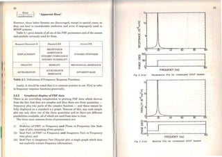
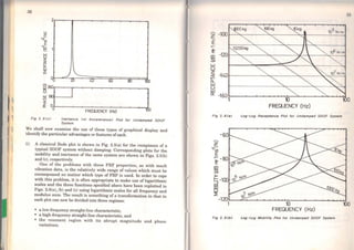
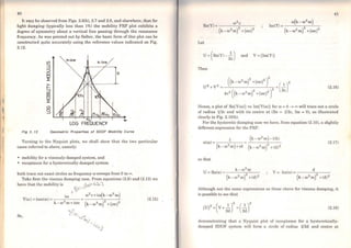
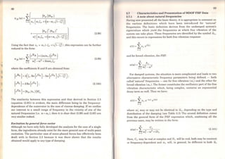
and they constitutc the basis of all our studies. Before leaving thc SDOF
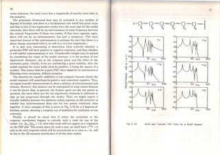
model, it is appropriate to consider Lhe forro which a ploL ofthe mobiliLy (of
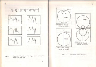
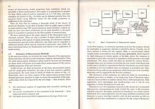
other type offrequency response function) takes. Three alternative ways of
plotting this information are shown in Fig. 1.1 and, as will be discussed
later, it is always helpful to select the format which is best suited to the
particular applicaLion to hand.
Ncxt we consider Lhe more general class of systems with more than one
degree-of-freedom. For these, it is customary that the spatial properties -
the values of the mass, stiffuess and damper elements which make up the
model - be expressed as matrices. Those used throughout this work are
[M], the mass maLrix, (K], the stiffness matrix, (C), lhe viscous damping
(a}
(b)
Fig , • 1
..!
1
1 o
...
1
~r--__
JO .., 00
'° 100
1 _]
~
g
1
i
1
~
f
>O 40 64 10 100
Pre:qu.tAC)' (HJ:•
10""'
10-J
10-~
~
V
10-• ~
""'10· • ~10 10 so 100
] 1 Q 1 1
10 lO
'º 100
ftlfqHncy Obl
Afternatlve Formets for Dlspfsy of Frequency
Functlon oi s Slngle-Degree-ol-Free·dom System
<s> Linear
<b> Logarfthmíc
9
Response](https://image.slidesharecdn.com/133501854-d-j-ewins-modal-testing-theory-and-practice-150524151503-lva1-app6891/85/133501854-d-j-ewins-modal-testing-theory-and-practice-13-320.jpg)
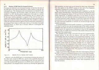
![1
}
lO
/m ( a/( ,./H l
Cl.0001
14.J ttr
- 0.0001
...."'
- 0.001
t•.J H.z •• ) ttr
FIQ 1. t <e> Nyqulst Plot
matrix, and [D), the structural or hysteretic damping matrix. The first
phase (of three) in the vibration ana1ysis of such systems is that of setting
up the governing equations of motion which, in effect, means determining
the elements of the above matrices. (This is a process which does exist for
the SDOF system but is often trivial.) The second phase is that of
performing a free vibration analysis using the equations of motion. This
analysis produces first a set of N natural frequencies and damping factors
(N being the number of degrees of freedom, or equations of motion) and
secondly a matching set of 'shape' vectors, each one of these bcing
associated with a specific natural frequency and damping factor. The
complete free vibration solution is conveniently contained in two matrices,
rÀ.2Jand [<l>], which are again referred to as the "modal prope:iies" or,
sometimcs, as the eigenva1ue (natural frequency and dampmg) and
eigenvector (mode shape) matrices. One element from the diagonal matrix
(Ã.2) contains both the natural frequency an d the damping factor for the
rth normal mode of vibration of the system whi1e the corresponding
column, {<>}r, from the full eigenvector matrix, [<I>], describes the shape
(the relative displacements of al1 parts of the system) of that sarne mode of
vibration. There are many detailed variations to this general picture,
depending upon the type and distribution of damping, but all cases can be
described in the sarne general way.
11
Tho third and fmal phase of theoretical analysis is the forced response ·
analysis, and in particular that for harmonic Cor sinusoidal) excitation. By
solving the equations of motion when harmonic forcing is app1ied, we are
able to describe the complete solution by a single matrix, known as the
"frequency response matrix" (H(co)], although unlike the previous two
matrix descriptions, the elements of this matrix are not constants but are
frequency-dependent, each element being itself a frequency response (or
mobility) function. Thus, element H jk (co) represents the harmonic
response in one of the coordinates, x j• caused by a single harmonic force
applied ata different coordinate, fk. Both these harmonic quantities are
described using complex algebra to accommodate the magnitude and
phase information, as also is H jk(e.o). Each such quantity is referred to as
a frequency response function, or FRF for short.
The particular relevance of these specific response characteristics is the
fact that they are the quantities which we are most likely to be able to
measure in practice. It is, of course, possible to describe each individual
frequency response function in terms of the various mass, stiffness and
damping elements of the system but the relevant expressioos are
extremely complex. However, it transpires that the sarne exprcssions can
be drastically simplified if we use the modal properties instead of the
spatial properties and it is possible to write a general expression for any
FRF, H jk (ro) as:
(1.1)
where À~ is the cigenvalue of the rth mode (its natural frequency and
damping factor combined;
~jr is the jth element of the rth eigenvector {~}r (i.e. the relative
displacement at that point during vibration in the rth mode);
N is the number ofdegrees offreedom (or modes)
This single expression is the foundation of modal testing: it shows a direct
connection between the modal properties of a system and its response
characteristics. From a purely theoretical viewpoint it provides an efficient
means ofpredicting response (by performing a free vibration analysis first)
while from a more practical standpoint, it suggests that there may be](https://image.slidesharecdn.com/133501854-d-j-ewins-modal-testing-theory-and-practice-150524151503-lva1-app6891/85/133501854-d-j-ewins-modal-testing-theory-and-practice-14-320.jpg)
![und ompliludc of lhe lcsl. lncorrecl transduccr sclcct1on cun ~ivc riso to
vory largc crrors in thc mcasured data upon which all thc subscqucnt
ana1ysis is based.
Tbe mobility parameters to be measured can be obtained directly by
applying a harmonic excitation and then measuring the resulting harmonic
response. This type of test is often referred to as 'sinewave testing' and it
requires the attachment to the structure of a shaker. The frequency range
is covered either by stepping from one frequency to the next, or by slowly
sweeping the frequency continuously, in both cases allowing quasi-steady
conditions to be attained. Alternative excitation procedures are now widely
used. Periodic, pseudo-random or random excitation signals often replace
the sine-wave approach and are made practical by the existence of cornplex
signal processing analysers which are capable of resolving the frequency
content of both input and response signals, using Fourier analysis, and
thereby deducing the mobi1ity pararneters required. A further extension of
this development is possible using impulsive or transient excitations which
may be applied without connecting a shaker to the structure. AH of these
latter possibilities offer shorter testing times but great care must be
exercised in their use as there are many steps at which errors may be
incurred by incorrect application. Once again, a sound understanding of
the theoretical basis - this time of signal processing - is necessary to
ensure successful use of these advanced techniques.
As was the case with the theoretical review, the measurement process
also contains many dctailed features which will be described below. Here,
we have just outlined the central and most important topics to
0
be
considered. One final observation which must be made is that in modal
testing applications of vibration measurements, perhaps more than many
others, accuracy of the measured data is of paramount importance. This is
so because these data are generally to be submitted to a range of analysis
procedures, outlined in the next section, in order to extract the resulta
eventually sought. Some of these analysis processes are themselves quite
complex and can seldom be regarded as insensitive to the accuracy of the
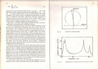
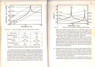
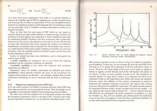
input data. By way of a note of caution, Fig. 1.4 shows the extent of
variations which may be obtained by using different measurement
techniques on a particular test strucl.ure [6].
1.6 Summary ofAnalysis
'l'he thírd skill rcquired for modal testing is concemed with the analysis of
the measured mobility data. This is quite separate from the signal
17
..... - - - - - - -1- - , - - . -T- 'f-,..-,
·-·-....
·-!
i
...
>000. 1o' ...000 • .o• "°°º.10• 6'000 110• .000 • 10
1 1-000 •IO'
,.,.,......c,11111
Fig t. 4 varlous Measurements on Standard Testplece
processing which may be necessary to convert raw measurem~~~s into
frequency responses. It is a procedure whereby the measured mob1hties are
analysed in such a way as to find a theoretical mod~l which m~st closely
resembles the behaviour of the actual testpicce. Th1s process itself falls
into two stages: first, to identify the appropriate type of model and second,
to determine the appropriate parameters of the chosen model. Most of the
effort goes into this second stage, which is widely referred to as
'experimental modal analysis'. .
We have seen from our review of the theoretical aspects that we ca~
'predict' or better 'anticipate' the form of the mobility plots for a multi-
degree-of-ft:eedom ~ystem and we have also seen that these ma~ b~ directly
related to the modal properties of that system. The great maJor1ty of ~he
modal analysis effort involves the matching or curve-fi.tting an express1on
such as equation (1.1) above to the measured FRFs and thereby finding the
appropriate modal parameters. . .
A completely general curve-fi.tting approach 1s poss1ble but generally
inefficient. Mathematically, we can take an equation of the form](https://image.slidesharecdn.com/133501854-d-j-ewins-modal-testing-theory-and-practice-150524151503-lva1-app6891/85/133501854-d-j-ewins-modal-testing-theory-and-practice-17-320.jpg)
![1
,, .
f
l
20
fiiLing - a set of modal propertios which bost match Lhe rot:!ponse
characteristics of the Lested structure. Some of thc more detuilcd
considerations include: compensating for slightly non-linear behaviour;
simultaneously analysing more then one mobility function and curve-
fitting to actual time histories (rather than the processed frequency
response functions).
1.7 Review ofTest Procedure
Having now outJined the major features ofthe three necessary ingredients
for modal testing, it is appropriate to end this introduction with a brief
review of just how these facilities are drawn together to conduct a modal
test.
The overall objective of the test is to determine a set of modal properties
for a structure. These consist of natural frequencies, damping factors and
mode shapes. The procedure consists ofthree steps:
(i) measure an appropriate set ofmobilities;
(ii) analyse these using appropriate curve-fitting procedures; and
(iii) combine the results ofthe curve-fits to construct the required model.
Using our knowledge of the theoretical relationship between mobility
functions and modal properties, it is possible to show that an 'appropriate'
set of mobilities to measure consists of just one row or one column in the
FRF matrix, (H(co)]. ln practice, this either means exciting the structure at
one point and measuring responses at ali points or measuring the response
at one point while the excitation is appJied separately at each point in tum.
(Tbis last option is most conveniently achieved using a hammer or other
non-contacting excitation device.)
In practice, this relatively simple procedure' will be embellished by
various detailed additions, but the general method is always as described
here.
..
21
CIIAPTER 2
Theoretical Basis
2.0 Introduction
It has already been emphasised that the theoretical foundations of modal
testing are of paramount importance to its successful implementation.
Thus it is appropriate that this first cbapter deals with the various aspects
of theory which are used at the different stages of modal analysis and
testing.
The majority of this chapter (Sections 2.1 to 2.8) deals with an analysis
of the basic vibration properties of the general linear structure, as these
form the basis of experimental modal analysis. Later sections extend the
theory somewhat to take account of the different ways in which such
properties can be measured (2.9) and some of the more complex features
which may be encountered (2.10). There are some topics of which
knowledge is assumed in the main text but for which a review is providcd
in the Appendices in case the current usage is unfamiliar.
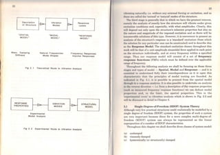
Before embarking on the detailed analysis, it is appropriate to put the
diíferent stages into context and this can be done by showing what will be
called the 'theorP.tical route' for vibration analysis (Fig. 2.1). This
illustrates the three phases through which a typical vibration analysis
progresses. Generally, we start with a description of the structure's
physical characte1;stics, usually in terms of its mass, stiffness and
damping properties, and this is referred to as the Spatial Model.
Then it is customary to perform an analytical modal analysis of the
spatial model which leads to a description of the structure's behaviour as a
set of vibration modes; the Modal Model. This model is defined as a set of
natural frequencies with corresponding vibration mode shapes and
modal damping factors. It is important to remember that this solution
always describes the various ways in which the structure is capable of](https://image.slidesharecdn.com/133501854-d-j-ewins-modal-testing-theory-and-practice-150524151503-lva1-app6891/85/133501854-d-j-ewins-modal-testing-theory-and-practice-19-320.jpg)

![42
(0, -1/2d) as illustrated in Fig. 2.ll(a).
2.3 Undamped Multi-Degree-of-Freedom (MDOF) System
Throughout much of the next six sections, we shall be discussing the
general multi-degree-of-freedom (MDOF) system, which might have two
degrees of freedom, or 20 or 200, and in doing so we shall be referring t.o
'matrices' and 'vectors' of data in a rather abstract and general way. ln
order to help visualise what some of these generalities mean, a specific
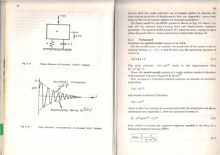
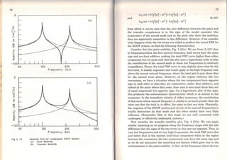
2DOF system, shown in Fig. 2.13, will be used although the general
expressions and solutions will apply to the whole range ofMDOF systems.
For an undamped MDOF system, with N degrees of freedom, the
governing equations ofmotion can be written in matrix formas
(M]{i(t)}+ (K]{x(t)} ={/(t)} (2.19)
where [M] and fK] are N x N mass and stiffness matrices respectively and
{x(t)} and {/(t)} are N x 1 vectors of time-varying displacements and
forces.
or
For our 2DOF example, the equations become
m 1i 1 +(k1 +k2)x1 -(k2)x2 =/1
m2i2 +(k2 +k3)x2 -(k2)x1 = !2
t-+X1 ....X2
k1 k2 ~
~),~,',,QFig 2. t 3 System wlth 2DOF Used as Example
m1 = t l<g m2 = t l<g l<t =1<3 =O. 4 MN/m
1<2 =O. 8 MN/m
or, using the data given in Fig. 2.13:
K =[ 1.2 - 0.8](MN/m)
-0.8 1.2
43
Wc shall consider first the free vibration solution (in order to determine
the normal or natural modal properties) by taking
{/(t)} ={O}
ln this case we shall assume that a solution exists of the forro
{x(t)} ={x}eiwt
where {x} is an N x 1 vector of time-independent amplitudes for which
case it is clear that {x} =- c.o2 {x}eimt.
(NOTE that this assumes that the whole system is capable of vibrating
ata single frequency, e.o.)
Substitution of this condition and trial solution into the equation of
motion (2.19), leads to
(2.20)
for which the only non-trivial solution is
(2.21)
or
from which condition can be found N values of c.o2
: (ro~, w~, ..., w;, ...,
w~), the undamped system's natural frequencies.
Substituting any one of these back into (2.20) yields a corresponding set
of relative values for {x}, i.e. {'l'}r, the so-called mode shape
corresponding to that natural frequency.
The complete solution can be expressed in two N x N matrices - th e
eigenmatrices - as
where (i)~ is the rth eigenvalue, or natural frequency squared, and {'I'}r is
a description of the corresponding mode shape.
Various numerical procedures are available which take the system](https://image.slidesharecdn.com/133501854-d-j-ewins-modal-testing-theory-and-practice-150524151503-lva1-app6891/85/133501854-d-j-ewins-modal-testing-theory-and-practice-30-320.jpg)
![44
matrices (M) and [K) (lhe Spatial Model), and convert them to the two
eigenmatrices rwn and ('1'] (which constitute the Modal Model).
It is very important to realise at this stage that one of these two
matrices - the eigenvalue matrix - is unique, while the other - the
eigenvector matrix - is not. Whereas the natural frequencies are fixed
quantities, the mode shapes are subject to an indeterminate scaling factor
which does not afTect the sbape of the vibration mode, only its amplitude.
Thus, a mode shape vector of
1
2
1
o
describcs exactJy the sarne vibration mode as
and so on.
3
6
3
o
What determines how the eigenvectors are scaled, or "normalised" is
largely governed by the numerical procedures followed by the
eigensolution. This topic will be discussed in more detail below.
For our 2DOF example, we find that equation (2.21) becomes
=ro4
(m 1m2)- ro2((m 1 +m2)k2+m 1k 3 +m2k 1)+(k1k 2+k1k3 +k2k3 )=O
Numerically
This condition leads to (i) ~ = 4 x 10⁵
(rad/s)2
and (i)~ = 2x 10⁶
(rad/s)2.
Substituting eit.hcr value ofinto the equation ofmotion, gives
or
45
Numerically, we have a solution
Before proceeding with the next phase - the response analysis - it is
worthwhile to examine some of the properties of the modal model as these
greatly influence the subsequent analysis.
The modal model possesses some very important properties - known as
the Ortbogonality properties - which, concisely stated, are as follows:
['P]T [M]('I'] = ['mrJ
('I')T (K]('I'] =('"krJ
(2.22)
from which: roo;J =l"mrJ-
1
['krJ where mr and kr are often referred to
as the modal or generalised mass and stiffness ofmode r. Now, because
the eigenvector matrix is subject to an arbitrary scaling factor, the values
of mr and kr are not unique and so it is inadvisable to refer to "the"
generalised mass or stiffness of a particular mode. Many eigenvalue
extraction routines scale each vector so that its largest element has unit
magnitude (1.0), but this is not universal. ln any event, what is found is
that the ratio of (k r/mr) is unique and is equal to the eigenvalue, (ron.
Among the many scaling or normalisation processes, there is one which
has most relevance to modal testing and that is mass-normalisation. The
mass-normalised eigenvectors are writ.ten as (Cl>) and have the particular
property that
and thus (2.23)
(Cl>f [K)[<I>]= ['ro;j
The relationship between the mass-normalised mode shape for mode r,](https://image.slidesharecdn.com/133501854-d-j-ewins-modal-testing-theory-and-practice-150524151503-lva1-app6891/85/133501854-d-j-ewins-modal-testing-theory-and-practice-31-320.jpg)
![1
46
{+}r' and its more general forro, fo/}r' is, simply:
(2.24)
or
A proof of the orthogonality properties is as follows. The equation ofmotion
may be written
(2.25)
For a particular modc, we have
(2.26)
Premultiply by a different. eigenvector, transposed:
(2.27)
We can also write
(2.28)
which we can transpose, and postmultiply by {'l'}'r, to give
(2.29)
But, since [M] and [K] are symmetric, they are identical t.o their
transposes and equat.ions (2.27) and (2.29) can be combined to give
(2.30)
which, if Wr -t:: @8 , can only be satisfied if
(2.31)
"7
Togcthcr wit.h cithcr (2.27) or (2.29), t.his mcans also that
(2.32)
For the special cases where r =s, equations (2.31) and (2.32) do not apply,
but it is clear from (2.27) that
({'li}; [K]{'li}r ) =w; ({'V}; (M]{'I'}r ) (2.33)
so that
and
Puttirlg together all the possible combinations of r and s leads to the full
matrix equation (2.22) abovc.
For our 2DOF example, the numerical results give eigenvectors which
are clearly plausible. Ifwe use them to calculate the generalised mass and
stiffness, we obtain
clearly
f-mrJ-11'-krJ =[ºo.4 o]06 r 2jL l 2.0 1 = Wr
To obtain the mass nonnalised version of these eigenvectors, we must
calcu]ate
[<J>]=[l l]r- j - 1/2 = [0.707 0.707]
1 - 1 IDr 0.707 --0.707](https://image.slidesharecdn.com/133501854-d-j-ewins-modal-testing-theory-and-practice-150524151503-lva1-app6891/85/133501854-d-j-ewins-modal-testing-theory-and-practice-32-320.jpg)
![1
1
48
Tuming now to a response analysis, we shall consider the case where
t.he structure is excited sinusoidally by a set of forces all at the sarne
frequency, Có, but with various amplitudes and phases. Then
a.nd, as before, we shall assume a solution exists of the form
{x(t)}= {x}ei(l)t
where {f} and {x} are N x 1 vectors of time-independent complex
amplitudes.
The equation of motion then becomes
([K]-ro2 [Ml){x} ei(l)l = {f} ei(l)t (2.34)
...
or, rearranging to solve for the unknown responses,
{x} =([K]-ro2
[MJr
1
{r} (2.35a)
which may be writtcn
{x} =[a(ro)]{f} (2.35b)
where [a(ro)] is the N x N receptance matrix for the system and constitutes
its Response Model. The general element in the receptance FRF matrix,
a jk (ro), is defincd as follows:
fm =O, m =1, N; i: k (2.36)
and as such represents an individual receptance expression very similar to
that defined earlier for the SDOF system.
It is clearly possible for us to determine values for the elements of[cx(ro)]
at any frequency of interest simply by substituting the appropriate va1ues
into (2.35). However, this involves the inversion of a system matrix at each
frequency and this has several disadvantages, namely:
• it becomes costly for large-order systems Oarge N);
49
• it i" i1uifTil'it11t 1f only u fow of tho individual FRF expressions are
r1'<1uirc•d;
• rt. prnvrdcs no insight into the fonn of the various FRF properties.
f"hr Lhcsc, and othcr, reasons an alternative means of deriving the various
Ji' U' pnramctcrs is used which makes use of the modal properties for the
''Yiilcm.
ltctuming to (2.35) we can write
(1 K]- ro2 [Ml) = (cxCro)r1 (2.37)
Prcmultiply both sides by [<t>]T and postmultiply both sides by [<l>] to
ohtain
or
,- '
(2.38)
It is clear from this equation that the receptance matrix [cx(ro)] is
symmetric and this will be recognised as the principie of reciprocity which
applies to many structural characteristics. lts implications in this situation
are that:
Equation (2.39) permita us to compute any individual FRF parameter,
ajk (ro}, using the following formula
(2.40)
..,
J](https://image.slidesharecdn.com/133501854-d-j-ewins-modal-testing-theory-and-practice-150524151503-lva1-app6891/85/133501854-d-j-ewins-modal-testing-theory-and-practice-33-320.jpg)
![50
or
which is very much simpler and more informative than by means of the
direct inverse, equation (2.35a). Here we introduce a new parameter, rAjk,
which we shall refor to as a Modal Constant: in this case, that for mode r
for this specific receptance linking coordinates j and k. (Note that other
presentations of the theory sometimes refor to the modal constant as a
'Residue' together with the use of'Pole' instead ofour natural frequency.)
The above is a most important result and is in fact the central relationship
upon which the whole subject is based. From the general equation (2.35a),
the typical individuaii FRF element a jk (ro), defined in (2.36), would be
expected to have the ~orm ofa ratio of two polynomials:
( )
- bo +b1co2 +b2co4 +... +bN- 1co2N-2
a jk (1) - 2 4 2N
a 0 +a1co +a2co +... +aNro
(2.41)
and in such a format it would be difficult to visualise the nature of the
function, a jk (co). However, it is clear that an expression such as (2.41) can
also be rewritten as
(2.42)
and by inspection of the form of (2.35a) it is also clear that the factors in
the denominator, (i)~, w~, etc. are indeed the natural frequencies of the
system, w; (this is because the denominator is necessarily formed by the
detI[K]- co2[MJI).
All this means that a forbidding expression such as (2.41) can be
expected to be reducible to a partial fractions series form, such as
(2.43)
Thus, the solution we obtain through equations (2.37) to (2.40) is not
51
unexpected, but ite eignifi.cance liee in the very simple and convenient
formula it provides for the coefficients, rAJ1t, in the series forro.
We can observe some of the above relationships through our 2DOF
example. The forced vibration equations ofmotion give
(k1 +k 2 -ro2m 1)x1 +·(- k2)x2 =f1
(-k2 )x 1+ (k2 + k s- ro2m2)x2 =f2
which,'in turn, give (for example):
(x1) k2 +ks - (1)2m2
Ti r2
=o =ro4
m1m2 - ro2((m1 +m2)k2 +m1ks +m2k1)
+(k1k2 + k2ks + k1ks)
or, nui:perically,
::
(o.sx 1012 - 2.4 x 10⁶ co2 + (1)4)
Now, if we use the modal summation formula (2.40) together with the
1results obtained earlier, we can write
2 2
(X, 11 =(~) = (l 4>1 ) + ( 2 $1 )
f1 w~ - 002 ro~ -(1)2
or, numerically,
0.5 0.5
= +~~~~~
0.4x 10⁶ -(1)2 2 x l 06 - co2
which is equal to (1.2 x 10⁶
-co2
)/(o.8x 10 12 -2.4 x 10⁶
(1)2 +ro4), as
above. •
The above characteristics of both the modal and response models of an
undam.ped MDOF system form the basis of the corresponding data for the
more general, damped, cases.
The following sections will examine the effects on these models of adding](https://image.slidesharecdn.com/133501854-d-j-ewins-modal-testing-theory-and-practice-150524151503-lva1-app6891/85/133501854-d-j-ewins-modal-testing-theory-and-practice-34-320.jpg)
![52
various types of damping, while a discussion of the presentation MDOF
frequency response data is given in Section 2.7.
2.4 Proportional Damping
ln approaching the more general case of damped systems, it is convenient
to consider first a special type of damping which has the advantage of
being particularly easy to analyse. This type ofdamping is usually referred
to as 'proportional' damping (for reasons which will be clear later) although
this is a soniewhat restrictive title. The particular advantage of using a
proportional damping model in the analysis of structures is that the modes
of such a structure are almost identical to those of the undamped version of
the model. Specifically, the mode shapes are identical and the nr.tural
frequencies are very similar to those of the simpler system also. ln effect, it
is possible to derive the modal properties of a proportionally damped
system by analysing in full the undamped version and then making a
· correction for the presence of the damping. While this procedure is often
used in the theoretical analysis of structures, it should be noted t~.~t it is
only valid in the case of this special type or distribution of damping, wº1'1ch
may not generally apply to the real structures studied in modal tests.
If we return to the general equation of motion for a MDOF system,
equation (2.19) and add a viscous damping matrix [C)we obtain:
[M){i} +[C){i}+[K]{x} ={!} (2.44)
which is not so amenable to the type of solution followed in Section 2.3. A
general solution will be presented in the next sectiop, but here we shall
examine the properties of this equation for the case where the darnping
matrix is directly proportional to the stiffness matrix; i.e.
[C) = P[K] (2.45)
(NOTE - It is important. to note that this is not the only type of
proport.ional damping - see below.)
ln this case, it is clear that if we pre- and post-multiply the damping
matrix by the eigenvector matrix for the undamped system ['1']' in just the
same way as was done in equation (2.22) for the mass and stiffness
matrices, then we shall find:
(2.46)
wl" 11i tlw daagonol clemcnts Cr reprcscnt the generalised damping of U1c
111 1111118 modcs of thc system. The fact that this matrix is also diagonal
111 " " " thut the undamped system mode shapes ar e also those of the
(11111111•d systcm, and this is a particular feature of tbis type of damping.
l l11MHlulcmcnt can easily be demonstrated by taking the general equation
111 111111to n above (2.44) and, for the case of no excitation, pre- and post-
1111111 aplying tbe whole equation by the eigenvector matrix, ['P]. We shall
1111•11 llnd:
{P}=pvr 1{x} (2.47)
1111111which the rth individual equation is:
(2.48)
ltit-h is clearly that of a single degree of freedom system, or of a single
11111tlo of the system. This mode bas a complex natural frequency with an
t• 111lntory part of
111111 11 dccay part of
(11•11 11g lhe notation introduced above for the SDOF analysis).
'l'hcse characteristics ca1Ty over to the forced response analysis in which
11 1mple extension ·or the steps detailed between equations (2.34) and (2.40)
11 (lcl~ to the definition for the general receplance FRF as:
I li
(2.49)](https://image.slidesharecdn.com/133501854-d-j-ewins-modal-testing-theory-and-practice-150524151503-lva1-app6891/85/133501854-d-j-ewins-modal-testing-theory-and-practice-35-320.jpg)
![54
which has a very similar form to that for the undamped system except that
now it becomes complex in the denominator as a result of the inclusion of
damping.
Gem?ral forms ofproportional damping
lt may be seen from the above that other distributions of damping will
bring about the sarne type of result and these are collectively included in
the classification 'proportional damping'. ln particular, if the damping
matrix is proportional to the mass matrix, then exactly the sarne type of
result ensues and, indeed, the usual definition of proportional damping is
that the damping matrix [C] should be ofthe forro:
[CJ =~(K)+ y(MJ (2.50)
ln this case, the damped system will have eigenvalues and eigenvectors as
follows:
' - - r:-r-2ror - Wr 'V 1- C.r
and
['f'damped ] =['f'undamped ]
Distributions of damping ofthe type described above are generally found
to be plausible from a practical standpoint: the actual damping
mechanisms are usually to be found in parallel with stiffness elements (for
internal material or hysteresis damping) or with mass elements (for
friction damping). There is a more general definition of the condition
required for the damped system to possess the sarne mode shapes as its
undamped counterpart, and that is:
(2.51)
although it is more difficult to make a direct physical interpretation of its
forro.
Finally, it can bc noted that an identical treatment can be made of a
MDOF system with hysterctic damping, producing the sarne essential
results. Ifthe general system equations ofmotion are expressed as:
55
IMl!d 1{IK1 iOJ){x} ={f} (2.52)
fiaul tht• hyslcrclic daroping matrix [D] is 'proportional', typically;
l'>J • MK)+y[M) (2.53)
t111, 11 we find that the mode shapes for the damped sy~tem are again
11 1, nlical to those of the undamped system and that the e1genvalues take
t li complex forro:
).,~ =ro; (l+ÍTlr) (2.54)
AIRo, the general FRF expression is written:
(2.55)
z.~ Hysteretic Damping - General Case
'l'hc analysis in the previous section for proportionally-damped sy~te~s
· · · ht m·to the characleristics of this more general descnptionit•vcs some ms1g
of practical structures. However, as was stated there, t~e c_ase ~f
proportional damping is a particular one which, although often JUStified m
11 theoretical analysis because it is realistic and also because º.f a lack ~f
uny more accurate model, does not apply to all cases. In our ~tudies here, 1t
ill very important that we consider the most general case if we are to be
uble to interpret and analyse correctly the data _we ?bserve on r~al
ttl ructures. These, after all, know nothing of our predil~ction for assum1~g
proportionality. Thus, we consider in the next two sections th~ properties
of systems with general damping elements, first ofthe hysteretic type, then
VIRCOUS.
W t rt by writing the general equation of motion for a MDOF system
e s a . h' h t
with hysteretic damping and harmonic excitation (as it is t is t a we are
working towards):
1M]{x}+[K]{x} +i[D] {x} ={f} eiwt (2.56)
Now, consider first the case where thet·e is no excitation and assume a
HOluLion ofthe forro:](https://image.slidesharecdn.com/133501854-d-j-ewins-modal-testing-theory-and-practice-150524151503-lva1-app6891/85/133501854-d-j-ewins-modal-testing-theory-and-practice-36-320.jpg)
![56
{x}={x}e1Ãt (2.57)
Substituted into (2.56), this trial solution leads to a complex eigenproblem
whose solution is in the form of two matrices (as for the earlier undamped
case), containing the eigenvalues and eigenvectors. ln this case, howevcr,
these matrices are both complex, meaning that each natural frequency and
each mode shape is described in ~rms of complex quantities, We choose to
write the rth eigenvalue as
(2.58)
where Wr is the natural frequency and llr is the damping loss factor for
that mode. It is important to note that the natural frequency Wr is not
(necessarily) equal to lhe natural frequcncy of the undamped system, Wri
as was the case for proportional damping, although the two values will
generally bc very close in practice.
The complex mode shapcs are at firsl more difficult to interpret but in
fact what we find is that the amplitude of each coordinate has both a
magnitude anda phase angle. This is only very slightly different from the
undamped case as lhere we eífectively have a magnitude at each point plus
a phase angle which is either Oº or 180°, both of which can be completely
dcscribed using real numbcrs. What the inclusion of general damping
eífects does is to gcneralise this particular feature of the mode shape data.
This eigensolution can be seen to possess the sarne type of ortbogonality
properties as those demonstrated earlier for the undamped system and
may bc defi.ned by lhe cquations:
(2.59)
Again, the generalised mass and stiífness parameters (now complex)
depend upon the normalisation of the mode shapc vectors for their
magnitudes but always obey the relationship:
(2.60)
and here again we may define a set ofmass-normalised eigenvcctors as:
(2.61)
57
N111111•1·l""' 4•xample11 willi Btr uclural damping
t 11
11
lurthor numorical cxamples are included to illustrate the
t11
1
11111
rtc1rieticll of rnoro general dampcd systems, based on the following
li ll li" modcl:
Mcufol l
1111 0.5 kg
m 2 1.0 kg
m3 =1.5 kg
k 1 =k2 =k 3 =k 4 =k 5 =k6 =1.0xl0
3
N/m
C'UAO l(a) - Undamped
o
3352
o
[
0.464
[<1>] = 0.536
0.635
-0.218
-0.782
0.493
-1.318]
0.318
0.142
('u~c l(b)- Proportional structural damping (d j = 0.05k j•j = 1.6)
[
950(1+0.05i)
IÀ~J = o
o o ]3352(1+0.05i) o
o 6698(1+0.05i)o
[
0.464(0º) 0.218(180º)
!<1>) = 0.536(0º) 0.782(180º)
0.635 (Oº) 0.493 (Oº)
1.318(180º)]
0.318(0º)
0.142(0º)
<'nt1e l(c) - Non-proportional structural damping (d1=0.3k1,d2-s =O,
1,c. o. single damper between m 1 and ground)
[
957 (1+0.067i)
r1..~J = ºo
o o ]3354(l+0.042i) o
o 6690(1+0.078i)
[
0.463 (...{).5°)
1<I>) :: 0.537 (Oº)
0.636 (1.0º)
0.217(173º) 1.321(181º) l0.784(181°) 0.316(-6.7°)
0.492(-1.3º) 0.142(-3.1º)](https://image.slidesharecdn.com/133501854-d-j-ewins-modal-testing-theory-and-practice-150524151503-lva1-app6891/85/133501854-d-j-ewins-modal-testing-theory-and-practice-37-320.jpg)
![58
NOTES:
(i) Each mode has a di!rerent damping factor.
(ii) Ali eigenvector arguments within 10° of0° or 180º (i.e. the modes are
almost 'real').
Model 2
ms =1.05 kgm 1 =1.0 kg
m2 =0.95 kg k 1 =k2 = ks =k4 =k5 =k6 =l.Ox103 N/m
Case 2(a)---'- Undamped
[
999
[ro;j = ~
o
3892
o [
0.577
[<1>] = 0.567
0.587
--0.602
--0.215
0.752
NOTE: This system has two close natural frequencies.
Case 2(b) - Proportional structural damping (di =0.05kj)
['À~J = o[
999 (1+0.05i)
3892(1+0.05i) oo o lo
[
0.577 (Oº) 0.602 (180°)
[<l>]= 0.567(0°) 0.215(180°)
0.587(0º) 0.752(0°)
o 4124{1+0.05i)
0.552 (Oº) l0.827 (180°)
0.207 (Oº)
0.552]
--0.827
0.207
Case 2(c) -Non-proportional structural damping (d1 =0.3ki.d2_6 =O)
lÀ~j = o[
1006(1+ O.lOi)
3942(1+0.031i) oo o lo
[
0.578 (-4°)
[<l>] = 0.569(2°)
0.588(2º)
0.851(162º}
0.570 (101°)
0.848 (12°)
o 4067(1+0.019i)
0.685 (40°) l1.019(176°)
0.560 (-50°)
59
/•111 ,.,.,/ n•s1>01uw analysis
W, 111rn noxt to tho anulysis of forced vibration for the particular case of
111111111111ic cxcitution and response, for which the governing equation of
111111 ion is:
(2.62)
A" 1J11foro, a direct solution to this problem may be obtained by using the
t •111.1hons ofmotion to give:
{x} {[KJ+i[D]-(J)2(MJr
1
{f} = [a<(J))]{f} (2.63)
t.11 t ugain this is very inefficient for numerical application and we shall
111.1ko use of the sarne procedure as before by multiplying both sides ofthe
1·ci11ation by the eigenvectors. Starting with (2.63), and following the sarne
prnccdure as between equations (2.37) and (2.39), we can write:
(2.64)
.md from this full matrix equation we can extract any one FRF element,
Kuch as a jk ((J)) and express it explicitly in a series form:
I
N (ti>jr) (<hr )
(l 11. ((J)) = . 2
J" (J)2-(J)2+111(J)
r=l r r r
(2.65)
which may also be rewritten in various alternative ways, such as:
111•
111 these expressions, the numerator (as well as the denominator) is now
romplex as a result of the complexity of the eigenvectors. It is in this](https://image.slidesharecdn.com/133501854-d-j-ewins-modal-testing-theory-and-practice-150524151503-lva1-app6891/85/133501854-d-j-ewins-modal-testing-theory-and-practice-38-320.jpg)
![!l
'I
60
respe~t that the general damping case differs from that for proportional
dampmg.
Excitation by a general force vector
Having derive~ an expression for the general term in the frequency
response funct1on matrix exjk (ro), it is appropriate to consider next the
analysis o~ a situation where the system is excited simultaneously at
several pomts (rather than at just one, as is the case for the individual
FRF expressions).
The general behaviour for this case is governed by equation (2.62) and
the solution in (2.63). However, a more explicit (and perhaps useful) form
of this solution may be derived from (2.63) - although not very easily! _
as:
(2.66)
This equ~tio~ pcrmits the caJculation of one or more individual responscs
to an exc1tat1on ofsevera) simultaneous harmonic forces (ali ofwhich must
have the sarne frequency but may vary in magnitude and phase) and it
may be seen that the special case ofone single response to a single force (a
frequency response function) is clearly that quoted in (2.65).
Before leaving this section, it is worth mentioning another special case
of some interest, namely that where the excitation is a vector of mono-
phased forces. Here, the complete generality admitted in the previous
paragraph is restricted somewhat by insisting that ali forces have the sarne
frequency and phase, although their magnitudes may vary. What is of
interest in this case is to see whether there exi~t any conditions under
which it is possible to obtain a similarly mono-phased response (the whole
syste.m respond~ng with a single phase angle). This is not generally the
casem the solut1on to equation (2.66) above.
Thus, let the force and response vectors be represented by
{x} = {x} ei(Olt-e)
(2.67)
where both {F} and {x} are vectors of real quantities, and substitute these
61
11110 tho l'ctuntion ofmotion (2.62). 'I'his lcads lo a complex equation which
1 r111 Ili' eplit into real and imaginary parts lo give:
((-<1)2
(M) +(KJ)cose +(D)sin a){x} ={F}
((-w2(M] +[K])sin 0-(D] cosa){x} ={O}
(2.68)
'l'he second of this pair of equations can be treated as an eigenvalue
111 nblcm which has 'roots' 08 and corresponding 'vectors' {K}8
• These may
hu inserted back into the :first of the pair of equations (2.68) in order to
1• tublish the form of the (mono-phased) force vector necessary to bring
ubout the (mono-phased) response vector described by {K}8
• Thus we find
thnt. there exist a set of N mono-phased force vectors each of which, when
upplied as excitation to the system, results in a mono-phased response
rharacteristic.
lt must be notcd that t.his analysis is even more complicated than it
nppears at first, mainly because the equations used to obtain the above
rncntioned solution are functions of frequency. Thus, each solution
oblained as described above applies only at one specific frequency, ro8 •
However, it is particularly interesting to determine what frequencies must
be considered in order that the characteristic phase lag (0) between (ali)
the forces and (all) the responses is exactly 90 degrees. Inspection of
C'quation (2.68b) shows that if0 is to be 90°, then that equation reduces to:
(-ro2
(M)+(KJ){x} =O (2.69)
which is clearly the equation to be solved to find the undamped system
natural frequencies and mode shapes. Thus, we have the important result
that it is always possible to find a set of mono-phased forces which will
cause a mono-phased set of responses and, moreover, if these two sets of
mono-phased parameters are separated by exactly 90°, then the frequency
at which the system is vibrating is identical to one ofits undamped natural
frequencies and the displacement 'shape' is the corresponding undamped
mode shape.
This most important result is the basis for many ofthe multi-shaker test
procedures used (particularly in tbe aircraft industry) to isolate the
undamped modes ofstructures for comparison with theoretical predictions.
It is also noteworthy that this is one of the few methods for obtaining](https://image.slidesharecdn.com/133501854-d-j-ewins-modal-testing-theory-and-practice-150524151503-lva1-app6891/85/133501854-d-j-ewins-modal-testing-theory-and-practice-39-320.jpg)
![62
directly the undamped modes as almost all other methods extract the
actual damped modes of the system under test. The physics of the
technique are quite simple: the force vector is chosen so that it exactly
balances all the damping forces, whatever these may be, and so the
principle applies equally to other types ofdamping.
Postscript
It is often observed that the analysis for hysteretic damping is less than
rigorous when applied to the free vibration situation, as we have done
above. However, it is an admissible model of damping for describing
harmonic forced vibration and this is the objective of most of our studies.
Moreover, it is always possible to express each of the receptance (or other
FRF) expressions either as a ratio of two polynomials (as explained in
Section 2.3) or as a series of simple terms such as those we have used
above. Each of the terms in the series may be identified with one of the
'modes' we have defined in the earlier free vibration analysis for the
system. Thus, whether or not the solution is st.rictly valid for a free
vibration analysis, we can usefully and confidently consider each of the
uncoupled terms or modes as being a genuine characteristic of the system.
As will be seen in the next section, the analysis required for the general
case of viscous damping - which is more rigorous - is considerably more
complicated than that used here which is, in effect, a very simple extension
ofthe undamped case.
2.6 Viscous Damping - General Case
We tum now to a corresponding treatment for the case of general viscous
damping. Exactly the sarne introductory comments apply in this case as
were made at the beginning of Section 2.5 and the only difference is in the
specific model chosen to represent the damping behaviour.
The general equation of motion for a MDOF system with viscous
damping and harmonic excitation is:
(M]{x}+(C){i} +(K) {x} ={/} (2.70)
As before, we consider first the case where there is zero excitation in order
to determine the natural modes of the system and to this end we assume a
solution to the equations ofmotion which has the·form
{x}={x}eªt (2.71)
1
63
H11h1:1htuting this into the appropriatc cquation ofmotion givcs:
(s21M]+s[C) t-(K]){x} ={O} (2.72)
lho solution of which constitutes a complex eigenproblem, although one
with a somewhat different solution to that of the corresponding stage for
thc previous case with hysteretic damping. ln this case, there are 2N
f'igenvalues, sr (as opposed to N values of Â.~ before) but these now occur
in complex conjugate pairs. (This is an inevitable result of the fact that all
the coefficients in the matrices are real and thus any characteristic values,
or roots, must either be real or occur in complex conjugate pairs.) As
bcfore, there is an eigenvector corresponding to each of these eigenvalues,
but these also occur as complex conjugates. Hence, we can describe the
cigensolution as:
o.nd
(2.73)
It is customary to express each eigenvalue Sr in the form:
where C.t>r is the 'natural frequency' and Çr is the critical damping ratio for
that mode. Sometimes, the quantity C.t>r is referred to as the 'undamped
natural frequency' but this is not strictly correct except in the case of
proportional damping (or, ofcourse, of a single degree of freedom system).
The eigensolution possesses orthogonality properties although these,
also, are different to those of the earlier cases. ln order to examine these,
we first note that any eigenvalue/eigenvector pair satisfies the equation
(s~[M)+sr(C)+[KJ}{'l'}r ={O} (2.74)
and then we pre-multiply this equation by {'I'}! so that we have:
(2.75)
A similar expression to (2.74) can be produced by using À.q and {'!'}q:](https://image.slidesharecdn.com/133501854-d-j-ewins-modal-testing-theory-and-practice-150524151503-lva1-app6891/85/133501854-d-j-ewins-modal-testing-theory-and-practice-40-320.jpg)
![64
(s~(M]+sq(C]+(KJ){'l'}q ={O} (2.76)
which can be transposed, taking account of the symmetry of the system
matrices, to give:
(2.77)
If we now postmultiply this expression by {'V}r and subtract the result
from that in equation (2.75), we obtain:
(2.78)
and, provided sr and Sq are different, this leads to the first of a pair of
orthogonality equations:
(2.79a)
A second equation can be derived from the above expressions as follows:
Multiply (2.75) by Sq and (2.77) by sr and subtract one from the other to
obtain:
(2.79b)
These two equations - (2.79a) and (2.79b)- constitute the orthogonality
conditions of the system and it is immediately clear that they are far less
simple than those we have encountered previously. However, it is
interesting to examine the form they take when tpe modes r and q are a
complex conjugate pair. ln this case, we have that
sq =ror (-çr -i~1-çn (2.80)
and also that
(2.81)
Inserting these into equation (2.79a) gives
65
(2.82)
whcre { }H denotes the complex conjuge (Hermitian) transpose, from
which we obtain:
(2.83)
Similarly, inserting (2.80) and (2.81) into (2.79b) gives
(()~ {'V}~ [M]{'V}r + {'V}~ [K]{'V}r =O (2.84)
from which
(2.85)
ln these expressions, mr, kr and Cr may be described as modal I.°ªs~,
stiffness and damping parameters respectively although the meanmg is
slightly different to that used in the other systems.
Forced response analysis . .
ln this stage of the analysis, this case of general viscous dampmg agam
presents a more complex task. Returning to the basic equation, (2.70), and
assuming a harmonic response:
{x(t)} ={x}ei<Ot (2.86)
we can write the forced response solution directly as
{x} = ([K]-ro2[M]+iro[Cl)-l {f} (2.87)
but as in previous cases, this expression is not particularly con~enient for
numerical application. We shall seek a similar series expans1on .to that
which has been used in the earlier cases of undamped, proport1onally-
damped and hysteretically-damped systems but now we find that the](https://image.slidesharecdn.com/133501854-d-j-ewins-modal-testing-theory-and-practice-150524151503-lva1-app6891/85/133501854-d-j-ewins-modal-testing-theory-and-practice-41-320.jpg)
![111
66
eigenvalue solution presented in the above equations is not directly
amenable to this task. ln fact, it is necessary to recast the equations in
order to achieve our aim.
Define a new coordinate vector {y} which is of order 2N and which
contains both the displacements {x} and the velocities {x}:
{y} = .{X}
X (2Nxl)
(2.88)
Equation (2.70) can then be written as:
[C: M)Nx2N {YJiNxl +(K: O]{y} = {O}Nxl (2.89)
However, in this form we have N equations and 2N unknowns and so we
add an identity equation of the type:
(M: O]{.Y}+[O : - M]{y} = {O} (2.90)
which can be combined to forma set of2N equations
(2.91a)
which can be simplified to:
(A]{.Y}+(B]{y} = {O} (2.91b)
These equations are now in a standard eigenvalue form and by assuming a
trial solution of the forro {y} ={y}est, we can obtain the 2N eigenvalues
and eigenvectors of the system, Â.r and {0}r, which together satisfy the
general equation:
(Â.r [A]+(B]){0}r ={O} r= 1, 2N (2.92)
These eigenproperties will, in géneral, be complex although for the same
reasons as previously they will always occur in conjugate pairs. They
possess orthogonality properties which are simply stated as
(e)T [A](0J = ['arJ
(0]T (B](0] =[ôrJ
and which have the usual characteristic that
r =1, 2N
67
(2.93)
(2.94)
Now we may express the forcing vector in terms of the new coordinate
system as:
{P}2Nxl ={~} (2.95)
and, assuming a similarly harmonic response and making use of the
previous development of a series forro expression of the response
(equations (2.34) to (2.40)), we may write:
l.~.} =2N {e};.{P}{e}r
.· L a (1co- s )
ICOX 2Nxl r =l T r
(2.96)
However, because the eigenvalues and vectors occur in complex conjugate
pairs, this last equation may be rewritten as:
l.~.}=±({e};.{P}{e}r +{e}: ~PJ{e:Ll·co 1 ªr (1co - sr) a (1co- s )1 x ~ r r
(2.97)
At tlris stage, it is convenient to extract a single response parameter, say
x j• resulting from a single force such as fk - the receptance frequency
response function exjk, and in this case, equation (2.97) leads to:](https://image.slidesharecdn.com/133501854-d-j-ewins-modal-testing-theory-and-practice-150524151503-lva1-app6891/85/133501854-d-j-ewins-modal-testing-theory-and-practice-42-320.jpg)
![lj
70
and ro;, except in some special cases. Table 2.3 summarises ali the
different cases which have been included.
7 •
Eqn. ~ Natural Frequency
Case for e D Free Forced
FRF (I)~ ro.
UNDAMPED 2.40 REAL, CONST. o - iii.ro.
PROP. HYST. 2.55 REAL, CONST. REAL, CONST. ro,. iii.
PROP. VISC. 2.49 REAL, CONST. REAL(ro) ro,.~1-Ç~ ro.
GEN. HYST. 2.65 COMPLEX, CONST. REAL, CONST. ro. ro,.
GEN. VISC. 2.99 COMPLEX(w) REAL(ro) w.~1- Ç~ Wr
-
Table 2.3 FRF Formulae and Natural Frequencies
2.7.2 Mobility and impedance parameters
In every case, the most important feature of the general expression in
(2.101) is its close relationship with the FRF expression for the much
simpler SDOF system, studied in detail in Section 2.1. We shall now
consider the properties of this type of function and then examine the
various means used to display the information it contains. It should be
emphasised that a thorough understanding of the forrn of the different
plots of FRF data is invaluable to an understanding of the modal analysis
processes which are described in Chapter 4.
First, we consider the various forms of FRF. As before, there are three
main alternatives, using displacement, velocity or acceleration response to
produce respectively receptance, mobility or inertance (or acceler~nce).
These three forros are interrelated in just the sarne way as described
earlier, so that we may write:
(Y(ro)] = iro[cx(ro)]
[A(ro)] = iro[Y(ro)]
= - ro2
[cx(ro)]
(2.102)
71
Howcvcr, thc FRF data of multi-degree-of-frcedom systems have a more
complex form than their SDOF counterparts and this may be seen from the
strict definition ofthe general receptance cljk which is:
fm = O, m = 1, N; m ~ k (2.103)
and it is the footnote qualification which is particularly important.
We saw in Sections 2.1 and 2.2 that there exista further three formats
for FRF data, these bcing the inverses ofthe standard receptance, mobility
and inertance and generally known as 'dynamic stiffness', 'mechanical
impedance' and 'apparent mass' respectively. Whereas with a SDOF
system there is no difficulty in using either one or its inverse, the sarne
cannot be said in the case of MDOF systems. It is true to say that for
MDOF systems we can define a complete set of dynamic stiffness or
irnpedance data (and indeed such data are used in some types of analysis),
but it is not a simple matter to derive these inverse properties from the
standard mobility typc as the following explanation demonstrates.
In general, we can determine the response ofa structure to an excitation
using the equation:
{x} = {v} = [Y(ro)]{f} (2.104a)
Equally, we can write the inverse equation using impedances instead of
mobilities, as:
{f}=[Z(ro)]{v} (2.104b)
The problem arises because the general element in the mobility matrix
( Yjk (ro)) is not simply related to its counterpart in the impedance matrix
(ZJ1c (ro)) as was the case for a SDOF system. Stated simply:
1
Y.ik (ro) =YJrj (ro) ~ - -
Z jk (ro)
(2.105)
and the reason for this unfortunate fact derives from the respective
definitions, which are:
..](https://image.slidesharecdn.com/133501854-d-j-ewins-modal-testing-theory-and-practice-150524151503-lva1-app6891/85/133501854-d-j-ewins-modal-testing-theory-and-practice-44-320.jpg)
![82
Summary
The purpose of this section has been to predict the forro which will be
taken by plots of FRF data using the different display formats which are in
current use. Although we may have a working familiarity with measured
FRF plots, the results shown above have been derived entirely from
consideration of the theoretical basis of structural vibration theory and the
exercise in so doing proves to be invaluable when trying to understand and
interpret actual measured data.
2.8 Complete and Incomplete Models
All the preceding theory has been concerned with complete models; that is,
the analysis has been presented for an N degree of freedom system with
the implicit assumption that all the mass, stiffness and damping properties
are known and that ali the elements in the eigenmatrices and the FRF
matrix are available. While this is a valid approach for a theoretical study,
it is less generally applicable for experimentally-based investigations
where it is not usually possible to measurc all the coordinates, or to
examine all the modes possessed by a structure. Because ofthis limitation,
it is necessary to extend our analysis to examine the implications of having
access to something less than a complete set of data, or model, and this
leads us to the concept ofa 'reduced' or incomplete type ofmodel.
As intimated, there are two ways in which a model can be incomplete -
by the omission of some modes, or by the omission of some coordinates (or
both) - and we shall examine these individually, paying particular
attention to the implications for the response model (in the form of the FRF
matrix). Consider frrst the complete FRF matrix, which is N x N:
and then suppose that we decide to limit our description of the system to
include certain coordinates only (and thus to ignore what happens at the
others, which is not the sarne as supposing they do not exist). Our reduced
response model is now of order n x n, and is written as:
Now, it is clear that as we have not altered the basic system, and it still
has the sarne number of degrees of freedom even though we have foregone
our ability to describe ali of them, the elements which remain in the
H:I
reduced mobility matrix are identical to the corresponding elemcnts in thc
full N x N matrix. ln other words, the reduced matrix is formcd simply by
extracting the elements ofinterest and leaving behind those to be ignored.
At this point, it is appropriate to mention the consequences of this type
of reduction on the impedance type of FRF data. The impedance matrix
which corresponds to the reduced model defined by [HR) will be denoted as
[ZR ] and it is clear that
(2.108)
It is also clear that the element.s in the reduced impedance matrix such as
Z~ are not the sarne quantities as the corresponding elemente in the full
impedance matrix and, indeed, a completely different impedance matrix
applies to each spccific reduction.
We can also consider the implications of this form of reduction on thc
other types of model, narnely the modal model and the spatial modeJ. For
the modal model, elimination of the data pertaining to some of the
coordinates results in a smaller eigenvecoor matrix, which then becornes
rectangular or order n x N. This matrix still retains N columns, and the
corresponding eigenvalue matrix is still N x N becausc we still have all N
modes included.
For the spatial model it is more difficult to cifcct a reduction of this type.
It is clearly not realistic simply to remove the rows and columns
corresponding to the eliminated coordinates from the mass and stiffness
matrices as this would represent a drastic change to the system. It is
possible, however, to reduce these spatial matrices by a number ofmethods
which have the effect of redistributing the mass and stiffness (and
damping) properties which relate to the redundant coordinates amongst
those which are retained. ln this way, the total mass of the structure, and
its correct stiffness properties can be largely retained. The Guyan
reduction procedure is perhaps the best known of this type although there
are several modelling techniques. Such reduccd spatial properties will be
denoted as:
Next, we shall consider the other form of reduction in which not ali the N
modes ofthe system are included. Frequently, this is a necessary approach](https://image.slidesharecdn.com/133501854-d-j-ewins-modal-testing-theory-and-practice-150524151503-lva1-app6891/85/133501854-d-j-ewins-modal-testing-theory-and-practice-50-320.jpg)
![84
in that many of the high frequency modes will be of little interest and
almost certainly very diffi.cult to measure. Considcr first the FRF matrix
and include initially all the coordinates but suppose that each element in
the matrix is computed using not all the N terms in the summation, i.e.:
(2.109)
ln full, we can thus write the FRF matrix as:
r( 2 2),r
1
T[Hfo>)]NxN =(<l>]Nxm Â.r -ü> ~mxm [<l>JmxN (2.110)
Of course, botb types of reduction can be combined when the resulting
matrix would be denoted:
[HR (ü>)]
nxn
Sometimes, it is convenient to attempt to provide an approximate
correction to the FRF data to compensate for the errors introduced by
leaving out some of the terms. This is usually effccted by adding a constant
or 'residual' term to each FRF, as shown in the following equation:
(2.111)
The consequence of neglecting some of the modes on the modal model is
evident in that the eigenvalue matrix becomes of order m x m and the
eigenvector matrix is again rectangular, althougli in the other sense, and
we have:
There is no immediate implication for the spatial type ofmodel ofomitting
some of the modes.
Fig. 2.23 shows the relationship between different forms ofcomplete and
inoomplete models.
~1·-· C
...
"'
li
85
~
<D
Ci.
E
o
()](https://image.slidesharecdn.com/133501854-d-j-ewins-modal-testing-theory-and-practice-150524151503-lva1-app6891/85/133501854-d-j-ewins-modal-testing-theory-and-practice-51-320.jpg)
![86
2.9 Non-Sinusoidal Vibration and FRF Properties
With receptance and other FRF data we have a means of computing the
response of a MDOF system to an excitation which consists of a set of
harmonic forces of diffcrent amplitudes and phases but all of the sarne
frequency. In the general case, we can simply write
{x}ei0>t = [o:(ro)]{f}eiwt (2.112)
We shall now turn our attention to a range of other excitation/response
situations which exist in practice and which can be analysed using the
sarne frequency response functions. Also, we shall indicate how the FRF
properties can be obtained from measurements made during non-
sinusoidal vibration tests.
2.9.1 Periodic vibration
The first ofthese cases is that ofpcriodic vibration, in which the excitation
(and thus the response) is not simply sinusoidal although it does retain the
property of periodicity. Such a case is illustrated in the sketch of Fig.
2.24(a) which shows a sawtooth type of excitation and two of the responses
it produces from a system. Clearly, in this case there is no longer a simple
relationship between the input and the outputs, such as exists for
harmonic vibration where we simply need to define the amplitude and
phase of each parameter. As a result, any function relating input and
output in this case will necessarily be quite complex.
It transpires that the easiest way of computing the responses in such a
case as this is by means of Fourier Series. The basic principie of the
Fourier Analysis is that any periodic function (such as f0 (t), x 1(t) or
x2 ( t) in Fig. 2.24(a)) can be represented by a series of sinusoids of suitable
frequencies, amplitudes and phases, as illustrated in Fig. 2.24(b). (A more
detailed discussion of Fourier Series is given in Appendix 3). So
..
fo(t)= L oFn é»nt
n=l
21tn
(1) =--
n T (2.113)
Once a frequency decomposition of the forcing function has been obtained,
we may use the corresponding FRF data, computed at the specific
frequencies present in the forcing spectrum, in prder to compute the
corresponding frequency components ofthe responses ofinterest:
87
X1(t) ~ X2(t)N-.,'
,~, '
T T
lal
-
~· -~""
+
~A!vv•. -+
(b)
2TI'
'UJ= -, T
'UJí= l.1T'
T
VJ.=6lr
J T
r-=r--~ / ·,
)~ -+
+ +
Fig 2. 24 Perlodlc Slgnals and thelr Sinusoida/ Components
..Xj(t)= 2,o:jo<ron) oFn eiroot
n=l
21tn
(l)n =--
T
(2.114)
What must be notcd here is that although the response contains exactly
the sarne frequencies in its spectrum as does the forcing, the relative
magnitudes of the various components are different in the two cas~s
because the FRF data vary considerably with frequency. Thus, wc obtain
rcsponse time histories which are periodic with th.e sam~ p~riod as the
excitation but which have a quite different shape to it and, mcidentally, to
each other (see Fig. 2.24).
To derive FRF from periodic vibration
It is possible to determine a system's FRF properties from excitati.on .ª~d
response measurements when the vibration is periodic. To do th1s'. 1t 1s
necessary to determine the Fourier Series components of both the mput
force signal and of the relevant output response sign.al(s). Both of th~se
series will contain components at the sarne set of d1screte frequenc1es;
these being integer multiples of 2n/T, where Tis the fundamental ~riod.
Once these two series are available, the frequcncy rcsponse funcbon can](https://image.slidesharecdn.com/133501854-d-j-ewins-modal-testing-theory-and-practice-150524151503-lva1-app6891/85/133501854-d-j-ewins-modal-testing-theory-and-practice-52-320.jpg)
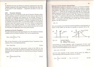
![90
This input/output relationship appears somewhat different to that
obtained via the Fourier Transform method, equation (2.117), but we shall
find that there is in fact a very dose relationship between them. This we
can do by using the Fourier Transform approach to compute the response
of a system to a unit impulse. Thus, let f(t) = ô(O) and determine its
Fourier Transform F(ro). ln this case, application of equation (2.115) is
relatively easy and yields:
F(ro) = 1/2n
If we now insert this expression into the general response equation,
(2.117), and note that, by definition, this must be identical to the impulse
response function, we obtain:
..
x(t) = h(t) = (1/2n) JH(ro) eirot dro (2.120)
Thus we arrive at a most important result in finding the Impulse and
Frequency Response Functions to constitute a Fourier Transform pair.
Following from this derivation, we can also see that the IRF can also be
expressed as a modal series, just as is possible for the FRF. Thus, if we
write
H(ro) = LHr (ro)
where Hr (ro) is the contribution for a single mode, we can likewise write:
where, for a viscously-damped system, hr (t) =Ar es,t.
To derive FRF. from transient vibration
As before, we are able to prescribe a formula for obtaining a structure's
FRF properties from measurements made during a transient vibration
test. What is required is the cakulation of the Fourier Transforms of both
the excitation and the response signals. The ratio of these two functions
(both of frequency) can be computed in order to obtain an expression for
the corresponding frequency response function:
1l(ro) =X(ro)
F(ro)
91
(2.121)
"ln practice, it is much more common to compute a Discrete Fourier
'l'ransform (DFT) or Series and thus to perform the sarne set ofcalculations
11s described in the previous section for periodic vibration. Indeed, such an
npproach using a DFT assumes that the complete transient event is
pcriodic.
Alternatively, the spectrum analyser may be used to compute the FRF
in the sarne way as it would for random vibration (see below), namely by
taking the ratio of the spectra. This is only useful if a succession of
repeated transients are applied - nominally, the sarne as each other - in
which case any noise on individual measurements will be averaged out.
2.9.3 Random vibration
We come now to the most complex type of vibration - where both
oxcitation .and response are described by random processes. Although it
might be thought that this case could be treated in much the sarne way as
the previous one - by considering the random signals to be periodic with
infinite period - this is not possible because the inherent properties of
random signals cause them to violate the Dirichlet condition. As a result,
neither excitation nor response signals can be subjected to a valid Fourier
Transform calculation and another approach must be found.
It will be necessary to introduce and define two sets ofparameters which
are used to describe random signals: one based in the time domain - the
Correlation Functions - and the other in the frequency domain - the
Spectral Densities. We shall attempt here to provide some insight into
these quantities without necessarily detailing all the background theory.
Considera typical random vibration parameter, f(t), illustrated in Fig.
2.26(a), which will be assumed to be ergodic. We shall introduce and define
the Autocorrelation Function Rtr (-t) as the 'expected' (or average) value of
the product (f(t).f(t+-t)), computed along the time axis.'This will always
be a real and even function oftime, is written:
Rff('t) = E [f(t).f(t+-t)] (2.122)
and will generally take the form illustrated in the sketch of Fig. 2.26(b).
This correlation function, unlike the original quantity f(t), does satisfy the
requirements for Fourier transformation and thus we can obtain its](https://image.slidesharecdn.com/133501854-d-j-ewins-modal-testing-theory-and-practice-150524151503-lva1-app6891/85/133501854-d-j-ewins-modal-testing-theory-and-practice-54-320.jpg)
![92
(o)
(b)
lc l
Fig 2. 26
f (t)
r
Ak.'LAJ
Baslc lngredlents oi Random S/gna/ Descrlptlon
<aJ Time Hlstory
<bJ Autocorrelatlon Functlon
<cJ Power Spectrel Denslty
Fourier Transform by the usual equation. The resulting parameter we
shall_ call a Spectral Density, in this case the Auto- or Power Spectral
Dens1ty (PSD), which is defined as:
..
Srr (w) = (1/27t) JRff (t) e-iM dt (2.123)
The ~uto-Spectral Density is a real and even function of frequency, and
does m .fact pro~de a frequency description of the original function f(t). It
has umts of (f /w) and would generally appear as in the plot of Fig. ,
2.26(c).
A similar concept can be applied to a pair of functions such as f(t) and
x(t) to produce cross correlation and cross spectral density functions. The
cross correlation function Rxr ('t) is defined as:
Rxf ('t) =E[x(t) .f(t+t)] (2.124)
93
und tho cross spcdral density (CSD) is defined as its Fourier Transform:
..
Sxr (w) = (1/27t) JRxr (t) e - im dt (2.125)
Cross correlation functions are real, but not always even, functions of time
and cross spectral densities, unlike auto spectral densities, are generally
complex functions of frequency with the particular conjugate property that:
S xr (w) =Srx (w) (2.126)
Now that we have established the necessary parameters to describe
random processes in general, we are in a position to define the
inputloutput relationships for systems undergoing random vibration. ln
deriving the final equations which permit the calculation of response from
known excitations, we shall not present a full analysis; rather, we shall
indicate the main path followed without detailing all the algebra. ln this
way, we hope to demonstrate the basis of the analysis and the origins of
the final expressions, which are the only ones required in normal modal
testing practice.
The analysis is based on the general excitation/response relationship in
the time domain, quoted above in equation (2.119) and repeated here:
..
x(t) = Jh(t - t')f(t')dt' (2.127)
Using this property, it is possible to derive an expression for x(t) and
another for x(t + t) and thus to caJcuJate the response autocorrelation,
Rxx ('t):
Rxx ('t) =E[x(t). x(t +t)] (2.128)
This equation can be manipulated to describe the response autocorrelation
in terms of the corresponding property of the excitation, Rff (t), but the
result is a complicated and unusable tripie integral. However, this sarne
equation can be transformed to the frequency domain to emerge with the
very simple form:](https://image.slidesharecdn.com/133501854-d-j-ewins-modal-testing-theory-and-practice-150524151503-lva1-app6891/85/133501854-d-j-ewins-modal-testing-theory-and-practice-55-320.jpg)
![li
11
,~I"
94
Sxx (ffi) = 1H(ro)j2 Srr ((1)) (2.129)
Although apparently very convenient, equation (2.129) does not provide a
complete description ofthe random vibration conditions. Further, it is clear
that it could not be used to determine the FRF from measurements of
excitation and response because it contains only the modulus of H((l)), the
phase information being omitted from this formula. A second equation is
required and this may be obtained by a similar analysis based on the cross
correlation between the excitation and the response, the frequency domain
form ofwhich is:
or, alternatively:
Srx ((1)) =H(ro)Sff ((1))
Sxx (ro) = H((l)) Sxr ((1))
(2.130)
So far, all the analysis in this section has been confined to the case of a
single excitation parameter, although it is clear that several responses can
be considered by repeated application of the equations (2.129) and (2.130).
In fact, the analysis can be extended to situations where severa!
excitations are applied simultaneously, whether or not these are correlated
with each other. This analysis involves not only the autospectra of all the
individual excitations, but also the cross spectra which link one with the
others. The general input/output equation for this case is:
[Srx ((l))] =[Srr (ro)] [H(ro)] (2.131)
To derive FRF from random vibration
The pair of equations (2.130) provides us with the basis for a method of
determining a system's FRF properties from the measurement and
analysis ofa random vibration test. Using either ofthem, we have a simple
formula for determining the FRF from estimates of the relevant spectral
densities:
or
H((l)) = Srx (ro)
Str (ro)
H(ro) = Sxx (ro)
Sxr (ro)
(2.132)
95
ln fact, the existcnce of two equations (and a third, if we include (2.129))
presente an opportunity to check the quality of calculations made using
measured (and therefore imperfect) data, as will be discussed in more
detail in Chapter 3.
2.10 Analysis Of Weakly Nonlinear Structures
2.10.1 General
Before concluding our review of the theoretical basis of the subject, it is
appropriate to include a consideration of the possibility that not ali the
systems or structures encountered in practice will be linear. All the
preceding analysis and, indeed, the whole basis of the subject, assumes
linearity, an assumption which has two main implications in the present
context:
(i) that doubling the magnitude of the excitation force would simply
result in a doubling of the response, and so on (response linearity
related to excitation), and
(ii) that if two or more excitation patterns are applied simultaneously
then the response thus produced will be equal to the sum of the
responses caused by each excitation individually (i.e. the principie of
linear superposition applies).
We shall now introduce some of the characteristics exhibited by weakly
(i.e. slightly) nonlinear systems, not in order to provide detailed analysis
but so that such structural behaviour can be recognjsed and identified if
encountered during a modal test. Thus we shall seek to derive and
illustrate the frequency response characteristics of such a system.
The equation of motion for a single degree of freedom system with
displacement and/or velocity dependant nonlinearity is:
m (x+2Ç ro0 i +w~ x +µ(x,x)) =/(t) (2.133)
This equation can be expressed as
m(x+~i+&~x) = f(t) (2.134)
where ~ and w~ depend on the amplitude (a) and frequency (ro) of
vibration, according to:](https://image.slidesharecdn.com/133501854-d-j-ewins-modal-testing-theory-and-practice-150524151503-lva1-app6891/85/133501854-d-j-ewins-modal-testing-theory-and-practice-56-320.jpg)
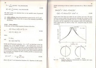
![Ili
li
~'
~I
li
98
2.10.3 Coulomb friction
In this case, we have a basic equation ofmotion ofthe type:
or
m(.x+2Çw0 i+wõ x)+ ~f =/(t)
m(x +ix+&Õ x}=/(t)=mF(t)
where
- 4R
À= 2Çw0 + ( )
,7,2 - ,.,2
""O - "'O
xaw0 m
(2.140)
(2.141)
Once again, a harmonic excitation will produce a more complex, though
periodic, response whose fundamenta] component is given by
x(t) .. a ei(J)t
where a is obtained from
((wÕ - w2
)
2
+(2Çw0 w)2
)a2 +(8Çw2 R/x)a
+((4Rw/x w0 )
2
- {f/m)2
) =O (2.142)
Further analysis of this expression shows that only a single value of a
applies. Plots of (a/f) for various values offand/or R are illustrated in Fig.
2.28.
~
'"'E
-
.D
o
:E
Fig 2. 28
o
20
Frequency !Hzl
99
Frequency Responso Characterlstlcs of System wlth Coulomb
Frlctlon](https://image.slidesharecdn.com/133501854-d-j-ewins-modal-testing-theory-and-practice-150524151503-lva1-app6891/85/133501854-d-j-ewins-modal-testing-theory-and-practice-58-320.jpg)
![,,
1
f
1
100
CHAPTER3
Mobility Measurement Techniques
3.0 Introduction
ln this chapter we shall be concerned with the measuremcnt techniques
which are used for modal testing. First, it is appropriate to consider
vibration measurcmcnt methods in general in order to view the context of
those used for our particular interest here. Basically, there are two types of
vibration mcasurcmcnt:
(i) those in whi.ch just one parameter is measured (usually a response
leve]), and
(ii) those in which both input and response output are measured.
Recalling the basic relationship:
1RESPONSE 1 = 1PROPERTIES 1 x 1INPUT 1
we can see lhat only when two of the three terms in this equation have
been measured can ,we define completely what is going on in the vibralion
of the test object. Ifwe measure only the response, then we are unable to
say whether a parLicularly large response leve! is dueto a strong excitati.on
or to a resonance of the structure. Nevertheless, both types of
measurement have their applications and much of the equipment and
instrumentation used is the sarne in both cases.
We shaJl be concerned here with the second type ofmeasurement, whcre
both excitation and rcsponse are measured simultaneously so that the
basic equation can be used to deduce the system properties directly from
the measured data. Within this category there are a number of different
approaches which can be adopted but we shall concentrate heavily on one
101
which we refer to as the 'single-point excitation' method. All the othcrs
involve simultaneous excitation at severa! points on the structure and
although we shall discuss these brieíly at the end of this chapter, our
interest will be focused on the more straightforward approach (at least
from the viewpoint of the experimenter) where the excitation is applied at
a single point (although in the course of a test, this point may be varied
around the structure). This type of measurement is often referred to as
'mobility measurement', and that is lhe name we shall use throughout this
work.
3.1 Basic Measurement System
The experimental set-up used for mobility measurement is basically quite
simple although there exista great many different variants on it, in terms
of the specific items used. There are three major items:
(i) an excitation mechanism,
(ii) a transduction syst,em (to measure the various parameters ofinterest,
and
(iii) an analyser, to extract the desired information (in the presence of the
inevitable imperfections which will accumulate on the measured
signals).
.--------.. Command
S.pal
Gtntrator
8 1
Allalyscr
Powtr
Amphíier
Sh~ker
Response
Transducers
Fig 3. 1 General Loyout oi Moblllty Meosurement System
Fig. 3.1 shows a typical layouL for the measurement system, detailing
some of the 'standard' items which are usually found. An additional
component has becn included in this illustration in the forro of a](https://image.slidesharecdn.com/133501854-d-j-ewins-modal-testing-theory-and-practice-150524151503-lva1-app6891/85/133501854-d-j-ewins-modal-testing-theory-and-practice-59-320.jpg)


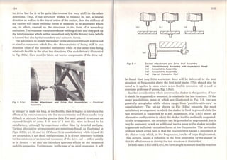
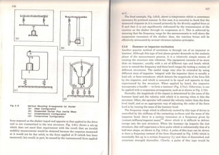
![118
Fig 3. l
f (t)
(a)
Fig 3. 8
Impactar snd Hsmmer Detalls
F(v..>)
t
(b)
100 Hz 1000
Typlcal lmpact Force Pulse and Spectrum
<a> Time Hlstory
(b) Frequency Spectrum
10 000
119
rnlutivoly inofioctivo ut cxciting vibrations in thc frcquency range above fc
1111d so we need to have some control over this parameter. It can be shown
lhnt thcro is a clirect relationship between the first cut-offfrequency fc and
lho duration of the pulse, Te, and that in order to raise the frequency
range it is necessary to induce a shorter pulse length. This in tum, can be
11con to be related to the stiffness (not the hardness) of the contacting
tiurfaces and the mass of the impactor head. The stiffer the materiais, the
shorter will be the duration of the pulse and the higher wiU be the
frequency range covered by the impact. Similarly, the lighter the impactor
mass the higher the effective frequency range. It is for this purpose that a
sct ofclifferent hammer tips and heads are used to permit the regulation of
the frequency range to be encompassed. Generally, as soft a tip as possible
will be used in order to inject all the input energy into the frequency range
of interest: using a stiffer tip than necessary will resu]t in energy being
input to vibrations outside the range of interest at the expense of those
inside that range.
On a different aspect, one of the difficulties of applying excitation using
a hammer is ensuring that each impact is essentially the sarne as the
previous ones, not so much in magnitude (as that is accommodated in the
force and response measurement process) as in position and orientation
relative to the normal to the surface. At the sarne time, multiple impacts or
'hammer bounce' must be avoided as these create difficulties in the signal
processing stage.
Yet another problem to be considered when using the hammer type of
excitation derives from the essentially transient nature of the vibrations
under which the measurements are being made. We shall return to this
characteristic later but here it is appropriate to mention the possibility of
inflicting an overload during the excitation pulse, forcing the structure
outside its elastic or linear range.
3.4 Transducers and Amplifiers
3.4.l General
The piezoelectric type of transducer is by far the most popular and widely-
used means of measuring the parameters of interest in modal tests. Only
in special circumstances are alternative types used and thus we shall
confine our discussion of transducers to these piezoelectric devices.
Three types of piezoelectric transducer are available for mobility
measurements - force gauges, accelerometers and impedance heads
(although these last are simply a combination of force- and acceleration-](https://image.slidesharecdn.com/133501854-d-j-ewins-modal-testing-theory-and-practice-150524151503-lva1-app6891/85/133501854-d-j-ewins-modal-testing-theory-and-practice-68-320.jpg)
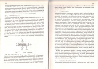
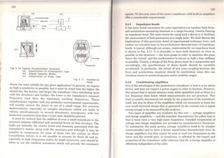
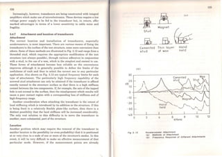
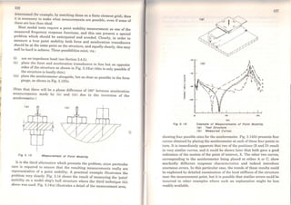

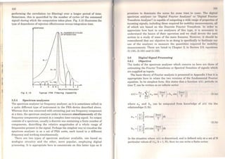
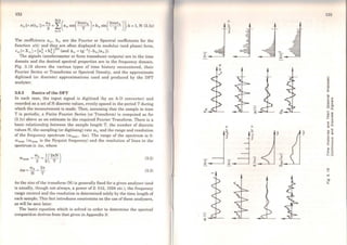
![134
X1 0.5 cos(27t/T)...
ªºxz 0.5 cos (47t/T)... ª1
X3 = 0.5 cos{6rt/T)... h1 or {xk} = [C]{a 0 } (3.4)
XN 0.5 cos(2N7t/T)
Thus, we use {a0 } =(Cr
1
{xk} to determine the unknown spectral or
Fourier coefficients contained in {an } • Much ofthe effort in optimising the
calculation of spectral analysis is effectively devoted to equation (3.4) and
the most widely uscd algorithm is the 'Fast Fourier Transform' developed
by Cooley and Tukey in the 1960s (Reference [7]). That rnethod requires N
to be an integral power of 2 and the va]ue usually taken is between 256
and 4096.
There are a number of features of digital Fourier analysis which, if not
properly treated, can give rise to erroneous results. These are generally the
result of the discrctisation approximation and of the need to limit the
length of the time history and in the following sections we shall discuss the
specific features of aliasing, leakage, windowing, zooming and
averaging.
3.6.3 Aliasing
There is a problem associated with digital spectral analysis known as
'aliasing' and this results from the discretisation of thc originally
continuous time history (Fig. 3.16). With this discretisation process, the
existence of vcry high frequencies in the original signal may well be
misinterpreted if the sampling rate is too slow. ln fact, such high
frequencies will appear as Jow frequencies or, rather, will be
indistinguishable from genuine low frequency cornponents. In Fig. 3.17, it
can be seen that digilising a 'low' frequency signal (Fig. 3.17(a)) produces
exactly the sarne set of discrete values as result frorn the sarne process
applied to a higher frequency signal, (Fig. 3.17(b)).
Tbus, a signal of frequcncy and one of (ro8 - ro) are indistinguishable
when rcpresented as a discretised time history and this fact causes a
distortion of the spectrum measured via the OFT, even when that is
cornputed exactly.
A signal which has a true frequency content shown in Fig. 3.18(a) will
appear in the DFT as the distorted form shown in Fig. 3.18(b). Note frorn
Section 3.6.2 that the highest frequency which can be included in the
spectrum (or transforrn) is (ro8 /2) and so the indicated spcclrurn should
(a)
(b)
Fig 3. , 7
(a)
( b)
Fig 3. 18
135
The Phenomenon of Aliasslng
u.is/2
Afias Olstortlon of Spectrum by Flnlte Fourier Translorm
(a) Actus/ Spectrum oi Slgnal
<bJ Spectrum lndlcated by Flnlte Trsnslorm](https://image.slidesharecdn.com/133501854-d-j-ewins-modal-testing-theory-and-practice-150524151503-lva1-app6891/85/133501854-d-j-ewins-modal-testing-theory-and-practice-77-320.jpg)
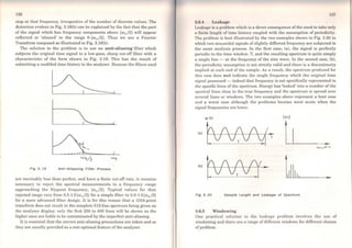
![138
w(t)
lolfJAP-•!.____~....._. ~ •
l•lfAA?·~. ~· ·
,,h ( ( ~ ~ I" ( ( ""' .., fV TV .. ..___li---~-- vVV
'"rvvv-~Fíg3.2t Dlfferent Types oi Wlndow
:X: (t)
~]'-
IXnl
UJn or n
Fig 3. 22 Effect ot Hannlna Wlndow on Finita Fourier Transform
Windowing involves the imposition of a prescribed profile on the time
signal prior to performing the Fourier transform and the profiles or
'windows' are generally depicted as a time function, w(t), as shown in Fig.
3.21. The analysed signal is x'(t) = x(t). w(t). The result of using a
Hanning or Cosine Taper window is seen in the third column of Fig. 3.21
and this in turn produces the improved spectrum shown in Fig. 3.22. The
Hanning (b) or Cosine Taper (e) windows are typically used for continuous
signals, such as produced by steady periodic or random vibration, while the
1:m
gxponential window (d) is used for transiont vibration applicationR wlwro
much of the import.ant information is conccntrated in thc initiol pnrt of tlw
time record and would thus be suppressed by either ofthe abovo choiccs.
3.6.6 Zoom
So far, we have been concemed with the basic DFT which is oftcn found to
have limitations ofinadequate frequency resolution, especially ai thc lowor
end ofthe frequency range and especially for lightly-damped systcms. This
problem arises because ofthe constraints imposed by the limitcd numbcr of
discrete points available (N), the maximum frequency range to be covcrcd
and/or the length of time sample available or necessary to provido good
data. An immediate solution to this problem would bc to use a largor
transform but, although giving finer frequency resolution around tho
regions of interest, this carries the penalty of providing more infonnation
than is required and, anyway, the size oftransform is seldom solectable.
The common solution is to 'zoom' in on the frequcncy range of intercsL
and to concentrate all the spectral lines (256 or 400 etc.) into a narrow
band between (J)min and Cl>max (instead of between o and (1) mnx. 08
hitherto). There are various ways of achieving this rcsult but porhaps tho
one which is easiest to understand physically is that which uAos 11
controlled aliasing effect. Suppose a signal x(t) has a spcclrum of lho ty1x-
shown in Fig. 3.23(a) and that we are intcrested in a dctoilNI {zoom)
analysis around the second peak - betwccn w1 and Cl)z.
ln ali cases, a rescaling is required to componsoto for tho 0Ut1nunlion of
the signals by the application of the window. How1.1
v<'r, if both rc.•sponsc and
excitation signals are subjected to the some window, und thc rcsulls are
used only to compensate a FRF ratio, thon lho rcHcnling is not nccessnry.
Care should be taken in some casos, cspcciolly wiLh transient testa, as tho
two signals may be treated differcntly.
Ifwe apply a band-pass filter to the sit,rnnl, as shown in Fig. 3.23(b), and
perform a DFT between O and (w2 - ooi), then bocause of lhe aliasing
phenomenon described earlier, thc frequcncy componcnts between ro1 and
w2 will appear aliased in the analysis range O-(w2 - ro1) (see Fig. 3.24)
with the advantage ofa finer resolution - in the example shown here, four
times finer resolution than in the original, baseband analysis.
When using zoom to measure FRF in a narrow frequency range, it is
important to ensure that there is as little vibration energy as possible
outside the frequency range of interest. This means that whercvcr
possible the excitation supplied to drive the structure should bo bund](https://image.slidesharecdn.com/133501854-d-j-ewins-modal-testing-theory-and-practice-150524151503-lva1-app6891/85/133501854-d-j-ewins-modal-testing-theory-and-practice-79-320.jpg)
![140
o
1
o
Fig 3. 23
o
Fig 3. 24
Ca>
eb>
Controfled Aflasslng for Frequency Zoom
<aJ Slgnal Spectrum
<bJ Band- Pass Fflter
'
r, ,' , ' V
Effectlve Frequency Translatlon for Zoom
limited to the analysis range; a feature not provided automatically on some
analysers.
As mentioned above, this is not the only way of achieving a zoom
measurement, but it serves to illustrate the concept. Other methods are
based on effectively shifting the frequency origin of the spectrum by
multiplying the original time history by a cos ro1 t function and then
filtering out the higher of the two components thus produced. For example,
suppose the signal to be analysed is:
14 1
x(t) = Asinwt
Multiplying this by cos ro 1 t yields
x '(t) =Asin rot cos w1 t =~ (sin (ro - ro 1 ) t +sin (ro +w1 ) t) (3.5)
and ifwe then filter out the second component we are left with the original
signal translated down the frcquency range by w1. The modified signal is
then analysed in the range O to (002 - wi) yielding a zoom measurement
between ro 1 and w2 ofthe original signal.
3.6.7 Averaging
We now turn our attention to another feature of digital spectral analysis
that concerns the particular rcquirements for processing random signals.
(So far, we have dealt with detcrministic data). When analysing random
vibration, it is not sufficient to compute Fourier transforms - strictly,
these do not exist for a random process - and we must instead obtain
estimates for the spcctral dcnsities and correlation functions which are
used to characterise this type of signal. Although these properties are
computed from the Fourier transforma, there are additional considerations
concerning their accuracy and statistical reliability which must be given
due attention. Generally, it is necessary to perform an averaging process,
involving several individual time rccords, or samples, before a result is
obtained which can be uscd with confidcnce. The two major considerations
which determine the number of averages rcquired are the statistical
reliability and the remova) of spu~us random noise from the signals.
Detailed guidance on the use of thcsc nnalyscrs for valid random signal
processing may be obtaincd from spccialist texts, such as Newland
(Reference [8]) and Bendat and Picrsol (Rcference [9)). However, an
indication of the requiremcnts from a statistical standpoint may be
provided by the 'statistical dcgrccs offrcedom' (11'.) which is provided by
lC =2BTt
where B =frequency bandwidth
Tt =total time encompassing ali data
(= mT for m samplcs cach ofT duration)
As a guide, this quantity K should be a minimum of 10 (in which case there](https://image.slidesharecdn.com/133501854-d-j-ewins-modal-testing-theory-and-practice-150524151503-lva1-app6891/85/133501854-d-j-ewins-modal-testing-theory-and-practice-80-320.jpg)
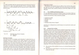
![146
curve results in the two cases, thcn there is a probability (though not an
assurance) that the sweep rate is not excessive.
It is possible to prescribe a 'correct' or optimum sweep rate for a given
structure, taking due account of its prevailing damping levels. ln theory,
any sweep rate is too fast to guarantee that the full steady state response
level will be attained, but in practice we can approach very dose to this
desired condition by using a logarithmic or similar type of sweep rate as
indicated by the graphs in Figs. 3.27(b), (c) and {d). Alternatively, the ISO
Standard (Refcrence (10]) prescribes maximum linear and logarithmic
sweep rates through a resonancc as follows:
Linear sweep
or
Smnx < 54 (fr )
2
(11r )
2
< 216 (fr )
2
(Çr )2
Hz/min
Logarithmic sweep
or
Smnx < 78 {fr )(rh )2
< 310{fr )(Çr )
2
octaves/min
Fig 3. 27
True Curve
"'•Oecreaslng t
Sweep l 1 .'
! .
;
:"-·',,...
lncreasing Sweep Rate
Freq.
FRF M9SSUr9m9nt by Sln9 SW99P Test
<sJ DlstortlnQ Effect of Sweep Rst9
.....
"O
..w
w
~li)
o
9
w
w!
ot-
< ..Ow
Ww
o~
-111
u
..w
w
~
li)
z
:i
w
w!
ot-
~ ..wW
o~
-111
147
N
=atzw
:::>
ow
a:...
o ...
- a:<...Ili
ã ti)
Q)
N <; Q) ~
=
Q) o
1- e: ~
> ~ cu Q)
a~
C> e: Q)
Q) o ~
:::> ~ ~ (/)
o (/) a: ~w
a:... ~2~... - e:~a: (/) ~ Q)
<... :.... =>E.,
~~ E
- - oe: - oQ) ::, Q)
E~ a:
Q) o
.... -g
~ Q)
s cu E ..._
Q) - ~
~ 1--...
la. ....... ..;
a: ~ o
14..-...-...
..... ã.o
......
.. (j
:I:
e?
~ >- OIu
z iÃ:
ªcr:
~ ~
i..
~j:!
92
iil~
o~
~g§
iii
~~ - u
~](https://image.slidesharecdn.com/133501854-d-j-ewins-modal-testing-theory-and-practice-150524151503-lva1-app6891/85/133501854-d-j-ewins-modal-testing-theory-and-practice-83-320.jpg)
![152
Ca>
eb>
Fia 3, 28
"'V
e
"'...
"'..e
o
u
...~
...
o
E- 20
"'..li)
"O
-; · l.0
g
o
...
"'e
- ·60
IM
o
I H,1
"H
os
100
Frequency IHzl
l'
,''~1 ~H1 .s.O
'"
"'JJ,""-.. ' s/'I •1
/li ~
li,' s/'1•10
''P11,
",I'
I I
' '
' ''! ,'
',
I
I
I
''
200
Cc)
0.1 ,-;-~--;:~:--=--~~---L--L.....l...--1_ _L_J
o1 0.2 o.s 1 2 s 10 20
fn'l/AI
50 100 200 soo 1000
FRF Messurement by Rsndom Excltstlon
<s> Modulus snd Coherence Plots
<b> Nyqulst Plots of Both FRF Estlmstes
<e) Msxlmum Error ln Resonsnce Pesk Estlmstes <l30])
153
(und thus data acquisit.ion time) is linked to the overall frequency
bandwidth.
Exactly how fine a frequency increment is required in order to reduce
this source of error to a minimum depends on severa! factors, including the
damping ofthe structure and the shaker/structure interaction discussed in
Section 3.3. Fig. 3.28(c) indicates the maximum error which might be
incurred in assuming that the true peak value of FRF is indicated by the
maximum value on the measured spectrum.
As a parting comment in this section on random excitation, we should
mention the need to make severa} successive measurements and to
accumulate a running average of the corresponding FRF estimates and
coherence. It is sometimes thought that a poor coherence can be eliminated
by taking a great many averages but this is only possible if the reason for
the low coherence is random noise which can be averaged out over a period
oftime. Ifthe reason is more systematic than that, such as the second and
third possibilities mentioned above, then averaging will not help. A
sequence of plots shown in Fig. 3.30(a) help to reinforce this point.
However, for these cases or frequency ranges where the coherence
genuinely reflects a statistical variation, then some guidance as to the
required number of averages for a given level ofconfidence can be obtained
from Fig. 3.31, based on the ISO Standard (Reference [10)).
Lastly, mention should be made here of a type of excitation referred to
as 'Periodic Random' which is, in fact, a combination of Pseudo Random
(Section 3.7.3) and 'Troe' Random. ln this process, a pseudo random (or
periodic) excitation is generated and after a few cycles, a measurement of
the input and the now steady-state response is made. Then, a different
pseudo random sequence is generated, the procedure repeated and the
result treated as the second sample in what will develop to be an ensemble
of random samples. The advantage over the simple random excitation is
that due to the essential periodic nature of each of the periodic random
samples, there are no leakage or bias crrors in any of the measurements.
However, the cost is an increase in the measurement time since %or %of
the data available is unused while steady response conditions are awaited
for each new sample.
3.7.5 Transient excitation
There are three types of excitation to be included in this section and they
are (i) the rapid sine sweep (or 'chirp', after the sound made by the input
signal), (ii) the 'burst' - a short section of signal (random or sine), and](https://image.slidesharecdn.com/133501854-d-j-ewins-modal-testing-theory-and-practice-150524151503-lva1-app6891/85/133501854-d-j-ewins-modal-testing-theory-and-practice-86-320.jpg)
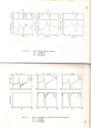
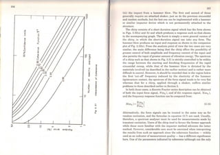
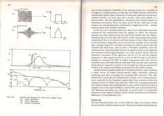
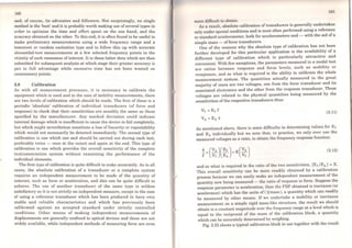
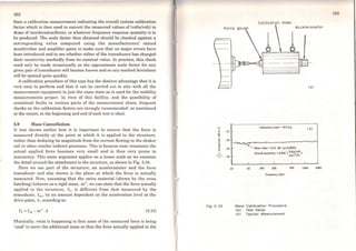
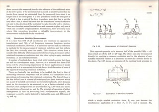
![168
(= -F1 .i1). A second test with the sarne excitation device applied at
position 2 gives a simultaneous excitation force Fo (= F2) and moment M0
(= F2 .i2). By adding and differencing the responses produced by these two
separate excitation conditions, we can deduce the translational and
rotational responses to the translational force and the rotational moment
separately, thus enabling the measurement ofall four types ofFRF:
X
F
e x e- and -
F' M M
The sarne principle can be extended to more directions by the use of a
multidimensional excitation fixture until the full 6 x 6 mobility matrix at
any given point can be measured. However, it must be noted that the
procedures involved are quite demanding, not least because they require
the acquisition of subsequent processing of many different measurements
made at different times.
Other methods for measuring rotational effects include specially
developed rotational accelerometers and shakers but in all cases, there is a
major problem that is encountered, which derives from the fact that the
prevailing levels of output signa] generated by the translational
components of the structure's movement tend to overshadow those due to
the rotational motions, a fact which makes the differencing operations
above liable to serious errors. For example, the magnitude of the difference
in equation (3.13) is often of the order to 1-2% of either of the two
individual values. When the transducers have a transverse sensitivity of
the order of 1-2%, the potential errors in the rotations are enormous.
Nevertheless, several applications of these methods have been quite
successful.
3.11 Measurements on Nonlinear Structures
Most of the theory upon which modal testing and mobility measurement is
founded relies heavily on the assumption that the test structure's
behaviour is linear. By this is meant that (i) if a given loading is doubled,
the resulting deflections are doubled and (ii) the deflection due to two
simultaneously applied loads is equal to the summation of the deflections
caused when the loads are applied one at a time. ln practice, real
structures are seldom compJetely linear although for practical purposes
many will closely approximate this state. However, there are many
complex structures which do behave in a nonlinear way and these can give
169
riso to concerns and problema when they are being tested.
Signs ofnonlinear behaviour include:
• natural frequencies varying with position and strength ofexcitation;
• distorted frequency response plots;
• unstable or unrepeatable data.
Perhaps the most obvious way of checking for nonlinearity is to repeat a
particular mobility measurement a number of times using different leveis
of excitation (and hence response) each time. If the resulting curves differ
from one such measurement to the next, especially around the resonances,
as illustrated in Fig. 3.38, then there is a strong possibility of nonlinearity,
and this is a check which will work with most types ofexcitation signal.
Fig 3. 38
z
~
E
41....
ll'.l
~
>..
·-
:ã
o
:!:
{ai
. .·.... ....
..;.
... ..
( b)
':.....
Example of Non-llnear System Response for Dlfferent
Excltatlon Leveis
<aJ Moblllty Modulus Plot
<bJ Receptance Nyqulst Plot](https://image.slidesharecdn.com/133501854-d-j-ewins-modal-testing-theory-and-practice-150524151503-lva1-app6891/85/133501854-d-j-ewins-modal-testing-theory-and-practice-94-320.jpg)
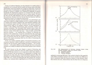
![172
responso function is related to the corresponding Imaginary Part by a
direct Hilbert transform.
Thus, ifwe have measurements ofboth parts (as is usually the case), we
can perform a check on the data by using the measured Real Part to
compute an estimate for the Imaginary Part and then comparing this with
the actual measured values. A similar comparison can also be made in the
other direction using the measured Imaginary Part to estimate the Real
Part. Differences between estimated and measured curves are then taken
as an indication of nonlinearity and the nature of the differences used to
identify which type. An example ofthe procedure is shown in Fig. 3.40 and
further details may be found in Reference [13). It must be noted that this
procedure will only work effectively if thc FRF data have been measured
using a sinusoidal excitation and care must be taken to avoid misleading
results which may arise if the data relate only to a limited frequency
range, thereby restricting the effectiveness ofthe Hilbert transform.
( bl-16.....J
~12o::
<a>
~8
;:;;! t.
~~~~--+,,.---~~
8
Fig 3. 40
3.12
_ 12
(!)
~ 8
=1.
~ Oi--~~---;.-t--~~~~~.....J
~ -1.
~-8.____........_,,.~~~....._~....__..
)J l.O 50 00 70 80
ffiEQJEflCY (RAOS/S)
Use of Hilbert Transform to Detect Non-llnearlty
<a> Effectlvely Linear System
<b> Non-llnear System
Multi·Point Excitation Methods
Although the great majority of modal tests are performed using a single-
point excitation procedure, it should be noted that there are other
approaches possible which make use of several simultaneously-applied
excitations. A detailed description of these alternative methods lies outside
t,hc scopc of this work although it is rccognised that they may be highly
suitable for certain specific applications, such as large aerospace type
structures. The theory upon which such multi-point excitation methods are
based has been presented in Chapter 2 and we shall briefly discuss here
the pracLical implementation of two rather different methods. A more
detailed account of these methods, and others of the sarne type, may be
found in Reference [29).
Il was shown earlier (equations (2.67) to (2.69)) that it is theoretically
possible to generate a monophased response vector by a multi-point,
monophased harmonic force vector, and furthermore that these two vectors
would be exactly 90° out of phase when the excitation frequency is equal to
one of the undamped system's natural frequencies. If we satisfy the
conditions posed in equations (2.67) to (2.69) where the force and response
vectors are exactly in quadrature with each other, then (2.63) may be
written as:
i{x} = (HRe(ro)+iHrm (ro)]{f} (3.16)
lt follows that this equation is valid only if det!Hne(ro)I =O and this
condition provides the basis of a method to locate the undamped system
natural frequencies from measured FRF data. A second stage - to find the
appropriate force vector - then follows by substitution of the specific
frequencies back into equation (3.16).
ln the case of the multi-point random approach, the purpose of the
method is to obtain the FRF data required for modal analysis but in a more
optimal way. Specifically, the aim of using severa} exciters simultaneously
is to reduce the probability of introducing systematic errors to the FRF
measurements, such as can arise when using conventional single shaker
methods. Once again, the underlying theory is presented in Chapter 2, this
time in equation (2.131). We shall consider the simplest form of a multiple
excitation as that of a system excited by two simultancous forces, f1 and
f2 , where t,he response Xi is ofparticular interest. Assuming that we have
measured the various auto and cross spectral densities of and between the
(three) parameters of interest, we can derive expression for the required
FRF parameters, Hn and Hi2:
(3.l7a)](https://image.slidesharecdn.com/133501854-d-j-ewins-modal-testing-theory-and-practice-150524151503-lva1-app6891/85/133501854-d-j-ewins-modal-testing-theory-and-practice-96-320.jpg)
![174
(3.17b)
These expressions can be used provided that 8 11 822 ~ IS12 l2
, a condition
which is more readily described by the requirement that the two excitation
forces must not be fully correlated. Care must be taken in practice to
ensure satisfaction of this condition, noting that it is the applied forces,
and not the signal sources, which must meet the requirement.
CHAPTER4
Modal Parameter Extraction
Methods
4.0 lntroduction
175
Having dealt with the first phase of any moda] test - that of measuring
the raw data from which the desircd mathematical model is to be derived
- we now turn our attention to the various stages of analysis which must
be undertaken in order to achieve the objectives. A major part of this
analysis consists of curve-fitting a theoretical expression for an individual
FRF (as developed in Chapter 2) to the actua] measured data obtained by
one of the methods discussed in Chapter 3. The present chapter dcscribes
some of the many procedures which are availablc for this task and
attempts to explain their various advantages and limitations: as with all
other aspects of the subject, no single method is 'best' for all cases.
ln increasing complexity, the methods discussed involve the analysis, or
curve-fitting, first of part of a single FRF curve, then of a complete curve
encompassing severa} resonances and, finally, of a set of many FRF plots
all on the same structure. ln every case, however, the task undertaken is
basically thc sarne: to find the coefficients in a theoretical expression for
the frequency response function which then most closely matches the
measured data. This task is most readily tackled by using the series form
for the FRF, as developed in Sections 2.3 to 2.6 for different types of
system. The particular advantage of this approach is that the coefficients
thus determined are directly related to the modal properties of the system
under test, and these are generally the very parameters that are sought.
This phase of the modal test procedure is often referred to as 'modal
analysis', or 'experimental modal analysis' because it is the corresponding
stage in an experimental study to that called modal analysis in a
theoretical study. ln both cases, modal analysis leads to a derivation of the](https://image.slidesharecdn.com/133501854-d-j-ewins-modal-testing-theory-and-practice-150524151503-lva1-app6891/85/133501854-d-j-ewins-modal-testing-theory-and-practice-97-320.jpg)
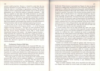
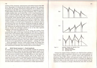
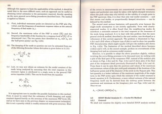
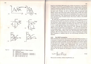
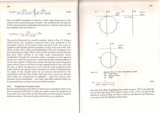
![186
lm(cr;) lm(oc)
Re (cr;) Re (oc)
Fig 4. 4 Propertles of Modal Clrcle
tany = llr
1-(w/wr)
2 (4.6a)
(ª) 1-(w/w )
2
tan (90° -y) = tan - = r
2 llr
(4.6b)
from which we obtain:
(4.6c)
Ifwe differentiate equation (4.6c) with respect to 0, we obtain:
f1f 2 21
dw2 -w; llr (1-(w/wr) ) _J
- = / (4.7)
d0 2 ll;
The reciproca] of this quantity - which is a measure of the rate at which
the locus sweeps around the circular are - may be seen to reach a
maximum value (maximum sweep rate) when w = Wri the natural
frequency of the oscillator. This is shown by further differentiation, this
time with respect to frequency:
~(dro
2
) =O when (w;-w2
) =O
dro da
187
(4.8)
It may also be seen from this analysis that an estimate of the damping is
provided by the sweep rate parameter since:
(
de ) 2
dro2 (l):(J)r = - w; llr
(4.9)
The above property proves useful in analysing MDOF system data since,
in general, it is not known exactly where is the natural frequency, but ifwe
can examine the relative spacing of the measured data points around the
circular are near each resonance, then we should be able to determine its
value.
Another valuable result can be obtained by further inspection of this
basic modal circle. Suppose we bave two specific points on the circle, one
corresponding to a frequency (rob) below the natural frequency, and the
other to one (roa) above the natural frequency. Referring to Fig. 4.4, we can
write:
tan(~) = 1-(rob/ror )2
2 llr
(4.10)
2
tan (~) = (roa /wr) - 1
2 llr
and from these two equations we can obtain an expression for the damping
ofthe mode:
w! - w~
llr =-------'----
w; (tan(0a/2) + tan(0b /2))
(4.11)
This is an exact expression, and applies for all levels of damping. Ifwe are
concerned with light damping (say, loss factors of less than 2-3%), the
expression above simplifies to:
(4.12)](https://image.slidesharecdn.com/133501854-d-j-ewins-modal-testing-theory-and-practice-150524151503-lva1-app6891/85/133501854-d-j-ewins-modal-testing-theory-and-practice-103-320.jpg)

![190
resonance, it is a relatively straightforward matter to devise an analysis
procedure to extract the necessary coefficients in equation (4.3a), and
thence the modal parameters themselves. Basing the following comments
on the case for structural damping, the sequence is:
(i) sclcct points to be used;
(ii) fit circle, calculate quality of fit;
(iii) locate natural frequency, obtain damping estimate;
(iv) calculate multiple damping estimates, and scatter;
(v) determine modal constant.
Step (i) can be made automatic by selecting a fixed number of points on
either side ofany identified maximum in the response modulus or it can be
effected by the operator whose judgement may be better able to discern
true modes from spurious perturbations on the plot and to reject certain
suspcct data points. The points choscn should not be iníluenced to any
great extcnt by the neighbouring modos and, whenever possible without
violating t.hat first ruie, should encompass some 270° of the circle. This is
oft.en not. possible and a span of lcss t.han 180º is more usual, although care
should be taken not to limit the range excessively as this becomes highly
sensitive to the accuracy of the few points used. Not less than six points
should be used.
The second step, (ii), can be performed by one ofnumerous curve-fitting
rout.ines and consists simply offmding a circle which gives a least-squares
deviation for the points included. Note that there are two possible criteria
which can be applied here: one is that which minimises t.he deviations of
points from the nearest point on the circle and the other, which is more
accurate, minimises the deviations of the measured points from where they
ought. to be on the circle. This latter condition is more difficult to apply and
so it is the former which is more common. At the end of this process, we
have specified the centre and radius of the circle and have produced a
quality factor which is the mean square deviation ofthe chosen points from
the circle. 'Errors' of the order to 1-2% are commonplace and an example of
the process is shown in Fig. 4.5(a).
Step (iii) can be implemented by constructing (here used metaphorically
as the whole process is performed numerically) radial lines from the circle
centre to a succession of points around the resonance and by noting the
angles they subtend with each other. Then, the rate of sweep through the
region can be estimated and the frequency at which it.reaches a maximum
Hll
can be deduccd. If, as is usually the case, the frcqucncies of the poinls uscd
in this analysis are spaced at regular intervals (i.e. a linear frequency
increment), then this process can be effected using a finite difference
method. Such a procedure enables one to pinpoint the natural frequency
with a precision of about 10% of the frequency increments between the
points. At the sarne time, an estimate for the daroping is derived although
this will be somewhat less accurate than that for the natural frequency.
Fig. 4.5(b) shows the results from a typical calculation.
It is interesting to note at this point that other definitions of the natural
frequency are sometimes used. Including:
(a) the frequency ofmaximum response:
(b) the frequency ofmaximum imaginary receptance;
(c) the frequency ofzero real receptance.
These are all indicated on the figure and while they seldom make a
significant difference to the va]ue of the natural frequency itself, selecting
the wrong one can have implications for the values found for the damping
factor and for the modal constant (and thus the mode shapes).
Next, for step (iv), we are able to compute a set of damping estimates
using every possible combination from our selected data points of one point
below resonance with one above resonance using equation (4.11). With all
these estimatcs we can either compute the mean value or we can choose to
examine thero individually to see whether thcre are any particular trends.
Ideally, they should all be identical and so an indication not only of the
mean but also of the deviation of the estimatcs is useful. Ifthe deviation is
less than 4-5%, thcn we have gcnerally succcedcd in making a good
analysis. If, however, the scatler is 20 or 30%, there is something
unsatisfactory. If the variations in damping estiroate are random, then the
scatter is probably due to measurement errors but if it is systematic, then
it could be caused by various effects (such as poor experimental set-up,
interference from neighbouring modes, nonlinear behaviour, etc.), none of
which should, strictly, be averaged out. Thus, if a large scatter of damping
estimates is indicated, a plot of their valucs such as that shown in Fig. 4.6
should be exaroincd.
Lastly, step (v) is a relatively simple one in that it remains to determine
the magnitude and argument of the modal constant from the diaroeter of
the circle, and from its orientation relative to the Real and Imaginary axcs.
This calculation is straightforward once the natural frequency has been](https://image.slidesharecdn.com/133501854-d-j-ewins-modal-testing-theory-and-practice-150524151503-lva1-app6891/85/133501854-d-j-ewins-modal-testing-theory-and-practice-105-320.jpg)
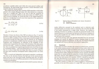
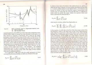
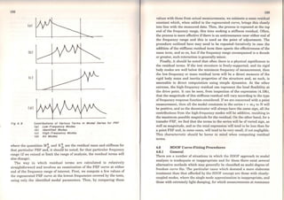
![202
[
m
2
A·k 1 1 ]m ( ) S J
o. (J) = +---
JK L w2 -w2 +iTt w2 KR w2 M~a=m 1 a a a jk Jk
..r
=-------(J)2 _ (J)2 +in (J)2
r •1r r
(4.22)
and we can use the sarne technique as before to obtain better estimates to
the modal parameters for mode r. This procedure can be repeated
iteratively for ali the modes in the range of interest as many times as is
necessary to obtain convergence to acceptable answers. It is often found
that on 'normal' FRF data, where most of the modes are relatively weakly
coupled, the improvement in the modal parameters is quite small - see
Fig. 4.10 for an example - but in cases where there is stronger coupling,
the enhancement can be significant.
4.6.3 Method 2: General curve-fit approach
The previous method was presented as it forms a natural development of
the earlier SDOF analysis method but it paves the way for more general
methods of MDOF curve-fitting. Many of the longer-established modal
analysis techniques were devised in the days of less powerful computation
facilities, and may, as a result, seem somewhat pedestrian by current
numerical analysis standards. However, they often have the advantage
than they permit the user to retain rather more direct contact with the
processes being used than would be the case in a more powerful, and
automatic algorithm. The secret is to maintain a balance between
computational sophistication on the one hand (-which might just be
thwarted by the relatively poor quality of the input data), and the lengthy
and often tedious practices which involve the user in many ofthe decisions.
However, we can describe the basics of a general MDOF curve-fit
philosophy, detailed implementation of which has been perfected by rnany
workers and made widely available. We shall denote the individual FRF
measured data as:
(4.23a)
while the corresponding 'theoretical' values are denoted by
z
~
'""E
Cll
....
Fig 4. 10
100
Frequency (Hz)
Comparlson of SDOF and MDOF Curve-Flts
300
(4.23b)
h th ffi . A ·k A ·k Rw ere e coe cients 1 J , 2 J , .. ., Wi. w2, ..., 111> Tt2 , .. ., K .k and
M~ are ali to be determined. We can define an individual erro/as et
where:
(4.24)
and express this as a scalar quantity:
(4.25)
if we further increase the generality by attaching a weighting factor wt to
each frequency point of interest, then the curve-fit process has to
determine the values of the unknown coefficients in (4.23) such that the
total error:](https://image.slidesharecdn.com/133501854-d-j-ewins-modal-testing-theory-and-practice-150524151503-lva1-app6891/85/133501854-d-j-ewins-modal-testing-theory-and-practice-111-320.jpg)
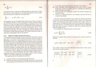
![206
{ajk (Q)} = (R]{Ajk } (4.30b)
from which a solution for the unknown modal constants r Ajk ir. terms v~
the measured FRF data points <Xjk (nt) and the previously identified
natural frequencies ror may·be obtained:
{Ajk } = (R)-1
{ajk (n)} (4.31)
An example of the application of the method is shown in Fig. 4.11 for an
-10
-120'--- ----L-----'----'---L----L- L--Jl,..._l-..L_ _ _ ___,
10 10 lo •o so 'º 10 ao 90 100 100
Frequency (Ht l
Fig 4. 11 MDOF Curve- Fft for L/ghtly Damped Structure
aerospace structure while further details ofits finer points are presented in
Reference (16). The performance of the method is found to depend upon the
points chosen for the individual FRF measuremeºnts, and these should
generally be distributed throughout the frequency range and, wherever
possible, should include as many antiresonances as are available. This last
feature has the particular advantage that at an antiresonance, the
theoretical model will exhibit a zero response: hence it is possible to supply
such a nil value for the appropriate data in equation (4.31). ln the limit,
this means that only one FRF data point may be required from the
measurements, all the others being set to be identically zero, even though
from the measurements on a real structure their values would be
extremely small, but finite.
207
4.7 MDOF Curve-Fitting in the Time Domain
4.7.1 Complex exponential method
As mentioned earlier in this chapter, there are a number of alternative
modal analysis methods which work on measured data in a time-domain
fonnat, rather than the more familiar frequency-domain versions. Most of
the available methods derive from a technique known as the 'complex
exponential' method, although there are several variants and refinements
which have been introduced in order to make the numerical procedures
more efficient and suitable for small computers. The basis of the method,
whose principal advantage is that it does not rely on initial estimates of
the modal parameters, is outlined below.
As the method uses the time-domain version ofsystem response data, in
the form of the Impulse Response Function, its present application is
limited to models incorporating viscous damping only. (It will be recalled
that the hysteretic damping model presents difficulties for a time-domain
analysis.) Our starting point is the expression for the receptance FRF of a
general MDOF system with viscous damping, which may be written as:
or
2N A
L
r jk
a. (ro) =Jk (l) y +i(ú> - ú), )
r=l r'>r r
(4.32b)
From dassical theory, we can obtain the corresponding Impulse Response
Function (IRF) by taking the Inverse Fourier Transform of the receptance:
2N
hjk(t)= IrAjk esrt (4.33)
r=l
If the original FRF has been measured, or obtained, in a digital form, and
is thus described at each of a number of equally-spaced frequencies, the
resulting IRF (found via thc Invcrse Fourier Transform of the FRF) will
similarly be described at a corresponding number of equally-spaced time](https://image.slidesharecdn.com/133501854-d-j-ewins-modal-testing-theory-and-practice-150524151503-lva1-app6891/85/133501854-d-j-ewins-modal-testing-theory-and-practice-113-320.jpg)

![210
2N- 1
:L~i hi =-h2N by setting ~2N = 1 (4.43)
i=O
and this may be written as
(4.44)
Now, we may repeat the entire process from equation (4.34) to equation
(4.44) using a different set of IRF data points and, further, we may chose
the new data set to overlap considerably with the first set - in fact, for all
but one item - as follows
(4.45)
Successive applications of this procedure lead to a.full set of 2N equations:
or
~o
~l
h4N-2 ~2N-l
from which we can obtain the unknown coefficients:
(4.46a)
(4.46b)
With these coefficients, we can now use (4.40) to determine the values Vi.
V2, ..., V2N from which we obtain the system natural frequencies, using
the relationship
211
Vr o•róL
We may now complete the solution by deriving the corresponding modal
constants, A1, A2, ..., A2N using equation (4.37). This may be written as
1 1 1 Ai ho
V1 V2 V2N A2 h 1
y2
1
y2
2 ViN Aa = h2
y2N- l
1
y2N-1
2
V2N- l
2N A2N h2N-l
or
[V]{A} = {h} (4.47)
Use ofcomplex exponential method
The foregoing method is generally employed in the following way. An
initial estimate is made for the number of degrees of freedom and the
above mentioned analysis is made. When completed, the modal properties
thus found are used in (4.32) to compute a regenerated FRF curve which is
then compared with the original measured data. At this stage, the
deviation or error between the two curves can be computed.
The whole procedure is then repeated using a different number of
assumed degrees of freedom (2N) and this error again computed. A plot of
error vs number of DOF will generally produce a result of the form shown
in Fig. 4.12 in which there should be a clearly-defined reduction in the
error as the 'correct' number of degrees of freedom is attained. The
inclusion ofa larger number than this critica} value will cause the creation
of a number of 'computational' modes in addition to the genuine 'physical'
modes which are ofinterest. Such additional modes serve to account for the
slight imperfection inevitably present in measured data and are generally
easily identified from the complete list of Vr and Ar modal properties by
their unusually high damping factors and/or small modal constants.
4.7.2 lbrahim Time-Domain method
Directly following the previous section on the complex exponential method,](https://image.slidesharecdn.com/133501854-d-j-ewins-modal-testing-theory-and-practice-150524151503-lva1-app6891/85/133501854-d-j-ewins-modal-testing-theory-and-practice-115-320.jpg)
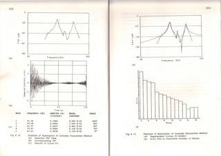
![214
it is appropriate now to introduce t.he lbrahim Time-Domain (ITD)
technique. Although the ITD method is not strictly a curve-fitting
procedure in the sense that all the preceding ones are and, indeed, it would
fü more readily into the next section, we shall present it here as a logical
extension ofthe complex exponential idea.
The basic concept of the ITD method is to obtain a unique set of modal
parameters - natural frequencies, damping factors and mode shapes -
from a set of free vibration measurements in a single analysis. ln other
words, we shall not be curve-fitting or analysing a single FRF (or
equivalent) at a time, as has been the case hitherto, but we shall be
processing ali the measured data at once. Another feature of the method is
that it can be used with any measured free vibration data, whether or not.
the excitation forces are available. ln the event that these data are known,
then it is possible to derive fully scaled eigenvector properties, otherwise
only the unscaled mode shapes will be available along with the modal
frequency and damping parameters. Perhaps the most likely way in which
the method will be applied in a modal testing context is by measuring a set
of FRF properties - based on a selection as prescribed in the next chapter
- and then by using these to obtain a corresponding set of Impulse
Response Functions. These may then be used as the free response data
required by the ITD method with the knowledge that the magnitude of the
excitation which produced them (a unit impulse) is implicit.
The theory of the method is as follows. As before, it is based on the free
vibration solution of a viscously-damped MDOF system and takes as its
starting point the assumption that we may write any individual response
as:
2m
Xj ( tj) = L('l'ir )esrt; (4.48)
r=l
where i represents the coordinate and j the specific time increment at
which the response is measured; Sr is the rth root or complex eigenvalue of
the system's characteristic equation (see equation (2.73)) and {'I'}r is the
corresponding eigenvector, with ('l'ir) being the jth element in that vector.
At this point, the eigenvectors are unscaled. Also, we are assuming that
the total number of degrees of freedom available in our model is m. ln fact,
this is not necessarily the sarne as the number ofdegrees of freedom of the
system (N): m is the number of degrees of freedom which are necessary to
represent the measured data and this may be possible with many less than
i tCí
the full set if, for example, the response is conílned to a limited frcqucncy
range, as will usually be the case in practice.
Now, if we measure the response at several points on the structure -
i =1, n - and at severa} instants in time - i =1, q - then we can
construct a matrix equation of the forro:
x1(ti) X1(t2) X 1 ( tq)
x2(ti) x2(t2) x2(tq)
=
Xn (t1) Xn (t2) Xn(tq)
11111 21111 2m111• 0 •1t1 eª•tq
11112 211'2 2m1112 eª2t1 e•2tq
(4.49a)
1vn 2"'" 2m'lln eª2mt1 eª2mtq
or, in simpler form:
(x] = ('I'](A)
(4.49b)
Here,
[x] is an n x q matrix of free response measurements from the structure,
and is known;
['I'] is an n x 2m matrix of unknown eigcnvcctor elcm~nts; and
[A] is a 2m x q matrix depending on the complex e1genvalues (as yet
unknown) and the response measurement times (which are known).
A second similar, equation is then formed by using a second set of
measured r~sponse data, each item of which relates to a time which is
exactly ~t later than for the first set. Thus we have:
2m
Xi(tt+ôt)= L('l'ir)esr(t,+ót} (4.50a)
r=l
or](https://image.slidesharecdn.com/133501854-d-j-ewins-modal-testing-theory-and-practice-150524151503-lva1-app6891/85/133501854-d-j-ewins-modal-testing-theory-and-practice-117-320.jpg)
![216
Xj(t,)= LN'ir)eªr(t,) (4.50b)
which leads to a second set ofequations:
(4.51)
Next, remembering that the number of assumed modes (m) is a variable
(we do not yet know how many modes are required to describe the observed
motion), we can arrange that n =2m, so that th~ matrices ['l'J and ["'l are
square. It may be seen that these two matrices are closely related ana we
can define a matrix [A]. often referrcd to as the 'system matrix', as:
(4.52)
From (4.49b) and (4.51). we find
[A][x] =[x] (4.53)
and this provides us with a means of obtaining [AJ from the measured
data contained in [xJ and [X.]. If we have selected the number of time
samples (q) to be identical to thc number of measurement points (n)
(~hich we have no~ set to be equal to 2m), then [AJ can be obtained
d1rectly from equation (4.53). However, it is customary to use more data
than the minimum required by sctting q to a value greater than 2m. In
~his case, use of equation (4.53) to determine [AJ will be via the pseudo-
mverse process which yields a least..squares solution for the matrix, using
all the data available. In this case, an expression for [A] is:
(4.54)
Returning now to equation (4.50). we can see that individual columns in
{'V}r are simply related to the corresponding ones in {jr} by the
relationship: r
(4.55)
Thus, using (4.52) we can write:
217
(4.56)
which will be rccognised as a standard forro of a sct of equations whose
solution is obtained by determining the eigenvalucs of the matrix [A]. It
must be noted immediately that these eigenvalues are not the same as
those of the original equations of motion (since equation (4.56) is not an
equation of motion) but they are closely related and we shall see that it is a
straightforward process to extract the system's natural frequencies,
damping factors and mode shapes from the solution to equation (4.56). The
cigenvalues of [A) are the particular values of (ea,Lt) and so ifwe have À.r
as one of thcse eigenvalues, thcn we can determine the corresponding
complex natural frequency ofthe system (sr) from:
(4.57a)
from which we can derive the natural frequency (ro1 ) and viscous damping
factor (Ç1 ) using
r =- ln(ª;+b;)(!)r ':>r 2ót
(4.57b)
ro' =ro ~1-r2 =tan-1 (br/ar)r r ':>r ót
Corresponding to each eigenvalue thcre is an eigenvector and this can be
seen to be ident.ica] to the modc shape vector for that mode. No further
processing is required in this case. It should, however, be noted that the
mode shapes thus obtained are generally unscaled and, as such, are
inadequate for regenerating FRF curves. Only if the original free vibration
response data were derived from a FRF-ffiF procedure can scaled (mass-
normalised) eigenvectors be obtained.
Use ofthe ITD method
As with other similar procedures, the ITD method requires the uscr to
make some decisions and judgements concerning which of his
measurements to use for the calculation (there will generally be an excess
of measured data). For example, there will often be more response points](https://image.slidesharecdn.com/133501854-d-j-ewins-modal-testing-theory-and-practice-150524151503-lva1-app6891/85/133501854-d-j-ewins-modal-testing-theory-and-practice-118-320.jpg)
![218
than there are genuine modes to be identified, but the method will always
produce one mode per two response points. Examination ofthe set ofmodal
properties, and especially the modal damping factors, will generally
indicate which are genuine structural modes and which are 'fictitious'
modes caused by noise or other irregularities in the measured data.
Various techniques are proposed for a systematic examination of the
results as the number of assumed degrees of freedom is increased.
Gcnerally, these methods look for a 'settling down' of the dominant modes
of vibration, or for a marked reduction in the least-squares error between
the original measured data and that regenerated on the basis of the
identified modal properties. Further details of the method, and its
sensitivity to various parameters are provided in reference [18).
4.8 Multi-Curve Fits (Global Curve-Fitting)
ln the next chapter we shall be discussing how results from the modal
analysis of several FRF plots for a given structure may be further
processed in order to yield the full modal model. At the present time,
having performed modal analysis on each of the individual frequency
responses, we have found the natural frequencies and damping factors but
wc do not yct have the mode shapes explicitly - only combinations of the
individual eigenvector elements as modal constants. A further stage of
processing is required - here referred to as 'modelling' - in order to
combine the various individual results obtained thus far. However, that
phase is somewhat anticipated by some of the more recent curve-fitting
procedures which are not confined to working with individual curves but
which are capable of performing a multi-curve fit. ln other words, they fit
severa! FRF curves simultaneously, taking due account of the fact that the
properties of all the individual curves are related by being from the sarne
structure. ln simple terms, all FRF plots on a given testpiece should
indicate the sarne values for natural frequency and damping factor ofeach
mode. ln practice, this does not happen exactly, unless they are
constrained to be identical, and in the next chapter we discuss ways of
dealing with this apparently unsatisfactory result. However, in a multi-
curve fü, thc constraints are imposed ab initio and such methods have the
advantage of producing a unique and consistent model as direct output.
One of the first published methods was that by Goyder [19], using an
extension of the frequency-domain method. Other methods, such as the
Ibrahim Time-Domain and one referred to as 'Polyreference' [20) are also
available.
iw
Anothcr way in which a set of measured FRF curves may bc utwd
collectively, rather than singly, is by the construction of a singlc composito
Response Function. We recall that
I
n rAjk
a (ro) =
J"k ro2 -ro2 +iro2T1
r=l r r r
(4.58)
and note that ifwe simply add several such FRFs, thus:
(4.59)
The resulting function HH(ro) will have the frequency and damping
characteristics of the structure appearing explicitly, just as does any
individual FRF, although the coefficients :I;1 (which replace the modal
constants) are now very complicated combinations of the mode shape
elements which depend heavily upon which FRFs have been used for the
summation. Nevertheless, the composite function HH(ro) can provide a
useful means of determining a single (average) value for the natural
frequency and damping factor for each mode where the individual
functions would each inclicate slightly diffcrent valucs.
As an example, a sct of mobilitics mcasured in a practical structure are
shown individually in Fig. 4.13(a) and thcir summation shown as a single
composite curve in Fig. 4.13(b). The results from nnalysis of the separate
curves produce estimates for the natural frcqucncy ond damping factor for
each mode, and these can be used to derive a menn value for each modal
parameter Also available are the uniquo vulucs for each parameter
produced by analysis ofthe single compositt> curve.
A similar property applies to the impulRe reRponse functions for use with
time-domain, rather than frequcncy clonwin, unalysis methods.
Both frequency-domain and time clomnin methods are amenable to the
expansion to multi-curve analyRiK. 'l'ho t.cchniques are simply quantitative
extensions of their single curv<' counterparts and have as disadvantages
first, the computation powor n•quirNl is unlikely to be available in an on-
line mini computer, and sccondly thnt there may be valid reasons why the
various FRF curves exhibit Kliuht diffcrences in their characteristics and it
may not always bc oppropriutc to average out all the variations.
Throughout the whoh• proccdurc of mobility measurements and modal](https://image.slidesharecdn.com/133501854-d-j-ewins-modal-testing-theory-and-practice-150524151503-lva1-app6891/85/133501854-d-j-ewins-modal-testing-theory-and-practice-119-320.jpg)
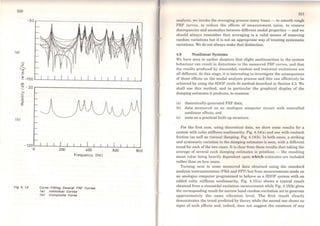
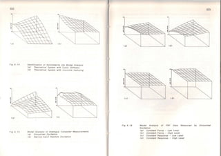


![228
which is formed from the mode shape data. ln order to extract the
'individual' elements of the mode shape matrix, [<l>], it is necessary to
made a series of measurements of specific frequency response functions
including, especially, the point mobility at the excitation position. If we
measure Hkk• then using (5.1) we see that analysis ofthis curve will yield
not onJy the natural frequency properties, but also the specific elements in
the mode shape matrix corresponding to the excitation point via:
r= l,m (5.2)
If we then measure any transfer FRF using the sarne excitation position,
such as Hjk• we are able to deduce the mode shape element corresponding
to the new response point using thc fact that the relevant modal constants
may be combined with those from the point measurement:
(5.3)
Hence we find that in order to derive a modal model referred to a
particular set of n coordinates, we need to measure and analyse a set of n
FRF curves, all sharing the sarne excitation point (or the same response
point, in the event that it is the excitation which is varicd) and thus
constituting one point and (n- 1) transfer FRFs. ln terms of the complete
FRF matrix, this corresponds to a requirement to measurc one column (or
one row, since the FRF matrix is gencrally symmetric), see Fig. 5.l(a). ln
practice, however, this requirement is the barest minimum of data which
will provide the necessary model and it is prudent to measure rather more
than a single column. Often, several additional elements from the FRF
matrix would be measured to provide a check, or to replace poor data, and
sometimes a complete second column or row might be advised in arder to
ensure that one or more modes have not been completely missed by an
unfortunate choice ofexciter location, see Fig. 5.l(b).
Once all the selected FRF curves have been measured and individually
analysed, using the most appropriate methods from Chapters 3 and 4,
there remains a further stage of processing to be done. Using any of the
singlc-curve modal analysis methods outlined in Chapter 4, we shall find
ourselves in possession of a set of tables of modal properties containing
rather more data than we are seeking. ln particular, we shall have
determined many separate estimates for the natural frequency and
Hu H12 Hli H1j HlN
H21 H22 H2i H2j H2N
Hi1 Hi2 Hii Hu HiN
Hj1 Hj2 Hji Hjj HjN
HN1 HN2 HNi HNj HNN
(a) Minimum Data Requirement
~ H12 H1i H1j H1N
H21
~ H2i R2j H2N
Hil Hi2 Ilii Hu HiN
Hj1 Hj2 HJI Hjj HjN
HN1 HN2 HN1 HNj IHNNI
(b) Typical Data Selcction
Fig 5. 1 Frequency Response Functlon Matrlx](https://image.slidesharecdn.com/133501854-d-j-ewins-modal-testing-theory-and-practice-150524151503-lva1-app6891/85/133501854-d-j-ewins-modal-testing-theory-and-practice-124-320.jpg)
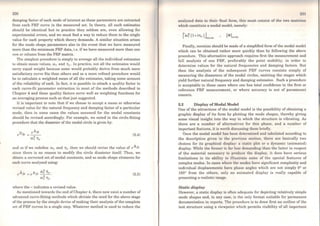
![232
points on the structure. Usually, this drawing is formed of a frame linking
the various coorclinates inc]uded in the modal survey, such as that shown
in Fig. 5.2(a) for a stiffened plate, and often this datum grid is drawn in
faint or broken lines. Then, the grid of measured coordinate points is
redrawn on the sarne plot but this time displaced in each direction (x, y
and z) by an amount proportional to the corresponding element in the
mode shape matrix. The elements in the matrix are scaled according to the
normalisation process used - and are usually mass-normalised - and
their absolute magnitudes have no particular significance in the present
process. It is customary to select the largest eigenvector element and to
scale the whole vector by an amount that makes that displacement on the
plot a viable amount. It is not possible to dictate how large a defiect.ion is
'viable' as this depends on the particular mode shape as well as on the
complexity of the st.ructural form itself. Itis necessacy to be able to sec how
the whole struct.urc deforma but t.he clisplacements drawn on the plot must
not be so Jarge that the basic geometry of the structure appears to be
violated. Fig. 5.2(b) shows a suitable plot for a mode ofthe plate previously
illustrated in 5.2(a).
ln this process, it. will be necessary to assign a positive or negative phase
to each element in the mode shape vector. Only phase angles which are
effectively Oº or 180° with respect to the norm can be accommodated on
this type of plot even though the results from the modal test may indicai.e
marked deviations from such a pattern. Thus, it is often necessary to
perform a 'whitewashing' exercise on the modal data and sometimes this
requires making difficult judgements and decisions, such as how t.o
incorporate an eigenvector element whose phase angle is closer to 90º than
to Oº or 180°. Fortunately, this dilemma is most often encountered on
modal deflections which are relatively small so that they do not influence
the overall shape of t.he plot very much. However, the selection ofpositive
or negative phase for such a point usually has the effect of determining t.he
location ofa nodal point or line, and this in itselfmay be important.
Dynamic display
The above-mentioned difficulties are avoided by the alternative display,
that of the animated mode shape. Using a suitable VDU and computation
facilities, it is possible to display on the screen a plot of the type just
described, and to update this picture at regular and frequent intervala of
time so that a simu]ation of the vibration is displayed in slow motion.
Usually what is done is that the coordinates for the basic picturc are
Fig 5. 2 Mode Shspe Plots
<sJ Bsslc Grld
<bJ Deformed Mode Shspe
<cJ Freeze- Frsme of Anlmsted Mode Shspe](https://image.slidesharecdn.com/133501854-d-j-ewins-modal-testing-theory-and-practice-150524151503-lva1-app6891/85/133501854-d-j-ewins-modal-testing-theory-and-practice-126-320.jpg)
![234
computed and stored, as are a corrcsponding set for a fraction of a
vibration cycle later, and then for a further fraction of a cycle later, and so
on. Each of these sets of data constitutes one 'frame' and some 10-20
frames are used for a complete cycle, i.e. at intervals of some 20º to 40° in
angular frequency. Once this data set has been constructed, successive
frames are displayed with an update rate which is suitable to give a clear
picture of the distortion of the structure during vibration; a rate which can
be adjusted to accommodate the varying phase angles of complex modes.
Another advantage of most animated mode shape displays is the additional
facility of changing the viewpoint from which the picture is drawn, often
necessary as different modes can be best viewed form different
orientations.
A static plot can be obtained from a dynamic display simply by 'freezing'
the animation (i.e. by requesting a zero update rate).
5.3 Response Models
There are two main requirements in the forro of a response model, the first
being that of regenerating 'theoretical' curves for the frequency response
functions actually measured and analysed and the second being that of
synthesising the other functions which were not measured. ln general, the
form of response model with which we are concerned is a FRF matrix
whose order is dictated by the number of coordinates included in the test.
(Note that this is not necessarily equal to the number of modes studied.)
Also, as explained in Section 5.1, it is not normal practice to measure and
analyse ali the elements in the FRF matrix but rather to select a small
fraction ofthese, usually based on one column or row with a few additional
elements included as a backup. Thus, if we are to construct an acceptable
response model it will be necessary to synthesise those elements which
have not been directly measured. However, in principle this need present
no major problem as it is always possible to compute the FRF matrix from
a modal model using:
~ fl( r 1
T
[H]nxn =[<f>]nxml 1À~ -ro
2
.l..Jmxm [<f>Jmxn (5.6)
Regenerated FRF curves
It is usual practice to regenerate a FRF curve using the resulta from lhe
modal analysis as a means of checking the success of that analysis, as
described in Chapter 4. However, if the collected results from severa! FRF
curves are subjected to an averaging process, such as that described in
Section 5.1, then a new regenerated curve should be produced and, if
necessary, a new set ofresiduals computed (see Section 4.4.). It should be
noted at this stage that in order to construct an acceptable response model,
it is essential that all the modes in the frequency range of interest be
included, as also are suitable residual terms to take account ofout-of-range
modes. ln this respect, the demands of the response model are more
stringent than those of the modal model.
Synthesis ofFRF curves
One of the implications of equation (5.6) is that it is possible to synthesise
the FRF curves which were not measured. ln simple terms, this arises
because if we measure three individual FRF curves such as Hik (ro),
H jk (ro) and Hkk (ro). then modal analysis of these yields the modal
parameters from which it is possible to generate. or 'synthesise' the FRF
Hij (ro), H ií(ro) etc. Indeed, application of this principie is sometimes
suggested as a means of checking the overall performance of a modal
analysis exercise.
However, it must be noted that there is an important limitation to this
procedure which can sometimes jeopardise the success of the whole
exercise. This limitation derives from the fact that only that part of the
relevant FRF which is due to the modes whose properties are available can
be computed. The remaining part, due to the out-of-range modes - the
residual part - is not available by this method of synthesis and, as a
result, a response model thus formed is liable to error unless values for the
relevant residual terms are available.
As an example, the result of applying this synthesis procedure to
measurements made on a turbine rotor are shown in Fig. 5.3. FRF data
H 11 and H 21> at and between the ends of the rotor, were measured and
analysed and the resulting modal parameters used to predict or
'synthesise' the other FRF H 22, initially unmeasured. This predicted curve
was then compared with measurements producing the result shown in Fig.
5.3(a). Clearly, the agreement is poor and would tend to indicate that the
measurement/analysis process had not been successful. However, the
'predicted' curve contained only those terms (in the complete modal series)
relating to the modes which had actually been studied from H 11 and H21
and this set ofmodes (as is oft.en the case) did not include all the modes of
the structure. Thus our predicted curve, H 22, omitted the influence of out-](https://image.slidesharecdn.com/133501854-d-j-ewins-modal-testing-theory-and-practice-150524151503-lva1-app6891/85/133501854-d-j-ewins-modal-testing-theory-and-practice-127-320.jpg)
![236
· 20
o
z,.....
~ -20
~
w
'O
-w - 40
u
z
~
Q:
w
~
-60
100
o
~ ·20
..-
""E
.,
~ - 40
(J)
'O
w
u
.z
<t
- -60Q:
w
.z
'ºº
Fig 5. 3
ea>
EXPERIMENTAL
CURVE
'•,
•
• I
~
( b)
..
'1
PREDICTED ~CURVE
,J
F REQUENCY (HZ)
PREDICTED
CURVE
•T
'
•
!" r1
I i 1
! , '
11 q
1f •
w
Ir
FREQU l: NCY {Hz)
Syntheslsed FRF Plot
1
1
•
•
o
<a> Uslng Measured Modal Data Only
<bJ Alter Addltlon oi Residual Terms
1 00
000
of-range modes or, in other words, lacked the residual terms. Thc inclusion
of these two additional terms (obtained here only after measuring and
analysing H 22 itself) resulted in the greatly improved predicted vs
measured comparison shown in Fig. 5.3(b).
The appropriate expression for a 'correct' response model, derived via a
set ofmodal properties is thus:
(5.7)
In order to obtain all the data necessary to form such a model, we must
first derive the modal model on which it is based (as described in Section
5.1) and then find some means of determining or estimating the elements
in the resid ual matrix, [R). This latter task may be most accurately
achieved by measuring all (or at least something over half) ofthe elements
in the FRF matrix, but this would constitute a major escalation in the
quantity of data to be measurcd and analysed. A second possibility, and a
reasonably practical one, is to extend the frequency range ofthe modal test
beyond that over which the model is eventually required. ln this way,
much of the contents of the residual terms is included in separate modes
and their actual magnitudes are reduced to relatively unimportant
dimensions. The main problem with this approach is that one does not
generally know when this last condition has been achieved althougb a
detailed examination of the regenerated curves using all the modes
obtained and then again less the highest one(s) will give some indications
in this direction.
A third possibility is to try to assess which ofthe many FRF elements are
liable to need large residual terms and to make sure that these are included
in the list of those which are measured and analysed. Wc noted earlier that
it is the point mobilities which are expected to have the highest-valued
residuais and the remote transfers which will have the smallest. Thus, the
significant terms in the [R] matrix will generally be grouped close to the
leading diagonal, and this suggests making measurements of most of the
point mobility parameters. Such a procedure would seldom be practical
unless analysis indicates that thc rcsponse model is ineffective without
such data, in which case it may be the only option.
Direct measurement
Finally on this topic, it should be noted that it is quite possible to develop a
response model by measuring and analysing all thc elements in one half of](https://image.slidesharecdn.com/133501854-d-j-ewins-modal-testing-theory-and-practice-150524151503-lva1-app6891/85/133501854-d-j-ewins-modal-testing-theory-and-practice-128-320.jpg)
![238
the FRF matrix (this being symmetric, only one half is essential) and by
storing the results of this process without constructing a modal model, or
'modal data base' as this is sometimes called. Such a procedure clearly
solves the residual problem discussed above but it is likely to present
another one by introducing inconsistencies into the model. Unless the
structural behaviour, the measurements and the analysis are ali of a
remarkable calibre, the small differences described in Section 5.1 will be
locked into the response model thus formed and will undoubtedly cause
serious difficulties when that model is put to use. At the very least, the
natural frequencies and damping factors of the individual modes should be
rationalised throughout the model but even that is insufficient to ensure a
satisfactory model.
Many of the sarne comments apply to the very crude method of obtaining
a response model by simply storing the raw measurements made of each of
the elements in the FRF matrix, a technique which bypasses the data
reduction and smoothing facilities afforded by modal analysis. Although
there are some instances where this is a viable procedure, they are rare
and rather special.
5.4 Spatial Models
It would appear from the basic orthogonality p'roperties ofthe modal model
that there exists a simple means of constructing a spatial model from the
modal model, but this is not so. From Section 2.3 we have that:
[<t>]T [M](<t>] =PJ
(<t>)T (K](<t>) =['1..~j
from which it would appear that we can write:
[MJ = [<t>rT [<t>rl
[KJ =[<t>rT [1..~Jr<t>rl
(5.8)
(5.9)
Indeed, we can, but this latter equation is only applicable when we have
available the complete N x N modal model. This is seldom the case and it is
much more usual to have an incomplete model in which the eigenvector
matrix is rectangular and, as such, is non-invertible. Even if we constrain
the number of modes to be the sarne as the number of coordinates (an
i:m
artificial and o~en impractical restriction) so that the matrix is squur<l, Uw
mass and stiffness matrices produced by equation (5.9) are mathcmatical
abstractions only and carry very little physical significance, unlcss n is
almost equal to N.
One step which can be made using the incomplete data is the
construction of 'pseudo' fiexibility and inverse-mass matrices. This is
accomplished using the above equations in the forro:
[K]-1 _(<t>) Í'I..2j-1 (<t>)Tnxn - nxm l r mxm mxn (5.10)
It is clear that a pair of pseudo matrices can be computed using the
properties of just a single mode. Further, it can be seen that the
corresponding matrices are simply the arithmetic sums of those for each
mode individually. Because the rank of each pseudo matrix is less that its
order, it cannot be inverted and so we are unable to construct stiffness or
mass matrices from this approach.
Further discussion on the construction of spatial models may be found in
the section concerned with the correlation of theory and experiment,
Section 6.2.
5.5 Mobility Skeletons and System Models
We have seen earlier how mobility and other FRF plots tcnd towards mass-
like or stiffness-like behaviour at frequencies well away from resonance
(and antiresonance). We have also suggested (in Scction 4.1), that a
'skeleton' of mass and stiffness lines can be constructed based on the FRF
curve and that this can be used to chcck the overall quality of the
measured curve. We shall now examine these skeletons in rather more
detail and show how they may be used to construct simple spatial models
ofa test structure.
We shall establish the basic features of thc skeleton using a very simple
mass-spring-mass 2DOF system, shown in Fig. 5.4(a) and for which the
point mobility Y11 has the forro shown in Fig. 5.4(b).
Certain basic features of this plot may bc predicted from knowledge of
the system, without necessarily computing the FRF in detail. These
features are that:](https://image.slidesharecdn.com/133501854-d-j-ewins-modal-testing-theory-and-practice-150524151503-lva1-app6891/85/133501854-d-j-ewins-modal-testing-theory-and-practice-129-320.jpg)
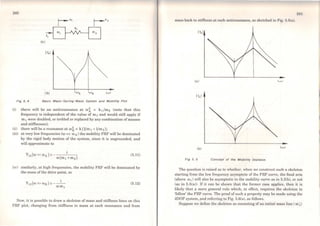
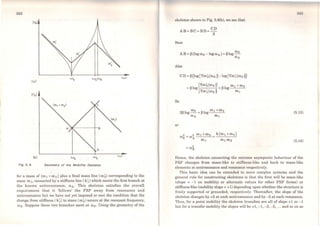
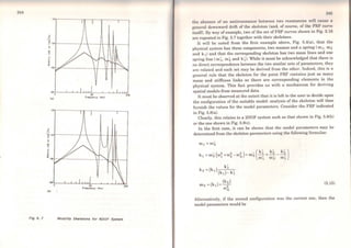
![246
(a)
(b)
Fig 5. 8
t,
m,
{e)
Moblllty Skeleton ot a 2DOF System
(a> Mobl/lty Curve and Skeleton
<b> Posslble System Conflguratlon
<e> Posslble System Conflguratlon
f1
m,
247
(5.16)
Hence the solution obtained is not unique and additional data would be
required in the example above in order to establish which of the two
configurations was the more representative. The additional data could be
provided by other FRF plots. ln his book, Salter [3] develops the skeleton
idea in greater detail, presenting a useful additional tool to the modal
analyst.](https://image.slidesharecdn.com/133501854-d-j-ewins-modal-testing-theory-and-practice-150524151503-lva1-app6891/85/133501854-d-j-ewins-modal-testing-theory-and-practice-133-320.jpg)

![250
6.1.2 Comparison ofresponse properties
If we start with the experimental model, we find that the raw data
available in this case are those describing the response properties of the
test structure since these are the only parameters we are able to measure
directly. For the predicted model, the response properties are those most
removed from the basic description of the structure and thus that require
the most efTort to produce. However, there are fewer uncertainties
introduced in the process of computing the frequency response properties
from the basic spatial model than arise in the alternative process (of
deriving a spatial model of the structure from test data) and so this is the
most appropriate form ofcomparison to be made in the first instance.
ln Fig. 6. l(a) we show the comparison between direct measurement and
prediction (via a finite element model) of a point FRF for a simple beam-
like structure. The plot clearly shows a systematic discrepancy between the
two scts of data (resulting in a steady frequency shift between the two
curves) while at the sarne time indicating a high dcgree of correlation in
the amplitude axis. Also of intercst are the relative values of the
frequcncies of resonance and of antiresonance, dose examination of which
can indicate whether the discrepancies are due to localised errors (loss of
stiffness at joints etc.) or to more general factors (such as incorrect values
ofelastic modulus or material density etc.).
A second example is shown in Fig. 6.l(b) where a transfer mobility for a
different structure is illustrated, again for both experimental and predicted
data. However, in this case the location of the response point used in the
modal test does not coincide exactly with any of the mcsh of grid points
used in the analytical model, thereby making a direct comparison
impossible. In order to proceed, the prcdicted curves relating the two grid
points closest to the tcst position (and these were only a few mm away, on
a plate-like structure of some lm x 2m) are used and are displayed in Fig.
6. l(b). ln this example, it is clear that not only are there marked
differences between the two models (albeit of a different type to the
prcvious case), but also there are striking differences between the two
predicted curves which relate to two points very dose to each other on the
structure. This last observation is very useful when we consider how to
assess the degrce of correlation betwcen the experimental and predicted
models. Because the particular parameter being measured (a FRF) can be
very sensitive to the exact location of the response point (and, possibly, to
the excitation point, although that does not suffer from the sarne difficulty
as does the response in the example cited), major differences may be
-Z4
~
z.....
1
CI)
E -48
CI>
...
m
"'O
-72
~
.D
o
~
- 96
-120
100
-60
~
z.....
1 -80
CI)
E
CI>
...
(]) -100
"'O
.D
o
~ -120
-140
100
Fig 6. 1
251
,•
'•
a
KEY
........ ME4SUREO
- - PREOICTEO
soo soo 700 900 1100 1300 1500
Frequency CHzl
b
KEY
MEASURCO ····- · POltlT :57
{
- l'Olllf 2
PREOICTEO ·-· POltlT :5
fOlCIHG rolllT li
200 :500 400 soo 600 700
Frequency eHzl
comparlson Between Measured and Predlcted Moblllty Data
<a> Polnt Moblllty for Beam Structure
(b) Transfer Moblllty for Plate Structure](https://image.slidesharecdn.com/133501854-d-j-ewins-modal-testing-theory-and-practice-150524151503-lva1-app6891/85/133501854-d-j-ewins-modal-testing-theory-and-practice-135-320.jpg)
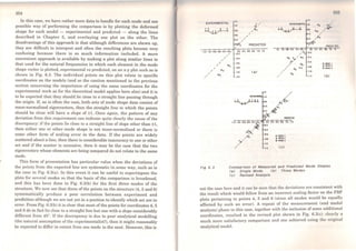
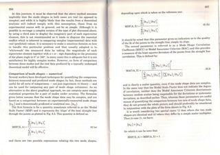
![r
258
and also that:
MAC(X,A)= 1
ln the second case, (ii), we have {~x} =r{~A} and we find that
MSF(X, A) = y while 1
MSF(A,X)=-
'Y
although, since the two modes are still almost perfectly correlated, we still
have:
MAC(X,A)= 1
In practice, typical data will be less ideal than this and what is expected is
that if the experimental and theoretical mode shapes used are in fact from
the sarne mode, then a value of the Assurance Criterion of close to 1.0 is
expected, whereas if they actually relate to two different modes, then a
value close to O.O should be obtained. Given a set of mx experimental
modes and a set of m A predicted modes, we can compute a matrix of mx x
mA Modal Assurance Criteria and present these in a matrix which should
indicate clearly which experimental mode relates to which predicted one. It
is difficult to provide precise values which the Assurance Criterion should
take in order to guarantee good results. However, it is generally found that
a value in excess of0.9 should be attained for correlated modes anda value
ofless than 0.05 for uncorrelated modes. However, the significance ofthese
quantities depends considerably on the subsequent use planned for the
model: some are much more demanding than others.
It is worth noting some of the causes of less-than-perfect results from
these calculations. Besides the obvious reason - that the model is
incorrect-values ofthe MAC ofless than unity can be caused by:
(i) nonlinearities in the test structure;
(ii) noise on the measured data; and
(iii) poor modal analysis of the measured data.
6.2 Correction or Adjustment ofModels
6.2.1 Rationale ofmodel adjustment
The next step to be considered is the possibility of extending any of the
comparison methods we now have available in order to correct or adjuat
one or other model. This procedure might set out to produce a re:fi.ned or
optimised set of measured properties (by making certain assumptions as to
which set are the more valid) or, alternatively, to adjust the theoretical
model in the light of the measurements.
The first step must be to make a rational decision as to which of the two
sets ofdata are to be taken as the reference (i.e. the more correct) set. This
decision will depend on several factors but will probably include
considerations based on the various comments above.
We shall describe four particular approaches which can be undertaken,
although the detailed procedures for each can vary. First, we shall examine
the possibility of assessing the validity of measured mode shapes by
checking their orthogonality through the theoretical mass matrix. The
second is a method for refining a measured set ofmode shapes, again using
the theoretical model mass matrix. The third (which is in effect a sequel to
the second) is a method for adjusting the theoretical model stiffness
matrix, once a refined set of mode shapes are available. The fourth
approach is for a method oflocating the regions in the mass and stiffness
matrices which harbour the greatest 'errors'. Although in theory these
methods could not only locate such errors but also quantify them, the
limitations imposed by the inevitable incompleteness of the measured data
mean that such an aspiration would be over-ambitious at present.
6.2.2 Orthogonality requirements
In this process, we extend the basic concept introduced above by
performing a calculation with the measured mode shapes and the
theoretical mass matrix. Ifwe compute:
(6.3)
We should obtain a unit matrix if the measured modes are indeed mass-
normalised and orthogonal with respect to the mass matrix. ln practice, it
would be necessary to have ensured the measurement of every coordinate
of the system and with a typical finite element model, this may well be
quite impractical. It is clear from the simple equation above that if even
only a few mode shape elements are omitted, the resulting o:thogonality
check is invalidated.
It is generally necessary, therefore, to obtain a reduced or condensed
mass matrix [M~] with which to perform the orthogonality check. The](https://image.slidesharecdn.com/133501854-d-j-ewins-modal-testing-theory-and-practice-150524151503-lva1-app6891/85/133501854-d-j-ewins-modal-testing-theory-and-practice-139-320.jpg)
![260
mass matrix must be condcnsed down l.o the sarno coordinat-0 set as has
been used in the modal test. Then, we can expect to find values of the
diagonal elements of the matrix produced by equation (6.3) in excess of 0.9
together with off-diagonal terms which are smaller than 0.05.
(NOTE: However, it should be noted that this procedure assumes that if
we take a condensed mass and stiffness matrix pair and compute their
eigenvalues and vectors, we shall find elements in the latter which are
identical to those for the corresponding coordinates in the eigenvectors for
the complete system model. lt is not obvious that this will indeed be the
case and so some caution should be used when drawing conclusions from
orthogonality checks of this type, especially where a significant
condensation or reduction has been carried out on the theoretical model
matrices.)
An altemative approach to the question of orthogonality check and one
which acknowledges the inevitable restriction on the number of elements
available in the measured eigenvector, involves both the theorctical mass
matrix and the corresponding stiffness matrix.
The basic equation:
is partitioned according to the measured elements (n) and the remainder
(s):
Mns]]{4>n} ={O}
Mas 4>a r
from which we have
so
{<l>s}Tsxl =-([Ksa]-ro;(Mss J)~~s ([Ksn ]- ro;(Msn l)sxn {4>n}Tnxl
=[Sr]sxn {4>n}r
(6.4)
(6.5)
Thus, the ort.hogonality check
{
= 1
=0
becomes
ifr= q
if r "# q
and can be computed from the theoretical mass matrix.
6.2.3 Adjustment of measured mode shapes
(6.6)
When we have made such a check on the measured modal properties, and
found them to be less than perfect, the question is raised as to what should
be done next. If it is decided that the measured data could be in error
(although not responsible for ali the discrepancies between experiment and
theory), then it is possible to derive an improved set of mode shapes by the
following procedure. It is necessary to assume that the adjustment to be
made is small and thus that the measured mode shapes are already good
estimates to the 'true' values. By this assumption we are justified in using
first-order terms (in the differences) only and it has been shown in
References [22) and [23) that an optimised set of measured mode shapes is
given by
(6.7)
where [<Dx) represents the measured modo shapes and (MA] the
theoretical mass matrix. ln this proceduro there aro two points to note.
First, we have not assumed that the predictod mode shapes are the correct
ones: we have only assumed that, tbe mass mal.rix part of the theoretical
model is correct and have not assigned any validity to the stiffness matrix.
The second point is that this procedure again requires us to have complete
data on each mode shape includcd. It is not strictly essential to include all
the modes but it is essential to incorporatc all the elements of those which
are included.
6.2.4 Adjustment of theoretical stiffness matrix
As a direct sequei to the previous method, we can now offer a rationale for](https://image.slidesharecdn.com/133501854-d-j-ewins-modal-testing-theory-and-practice-150524151503-lva1-app6891/85/133501854-d-j-ewins-modal-testing-theory-and-practice-140-320.jpg)
![262
adjusting the thcoretical model stiffness matrix (which, after all, is the
more likely one to contain errors). This is done on the basis of using the
refined measured mode shapes (see 6.2.3) together with the measured
natural frequencies, which will be taken as correct. The theory, which is
developed in References [22] and [23], is somewhat involved and derives
the only stiffness matrix which, together with the theoretical mass matrix,
will yield the measured eigenvalues and (adjusted) measured eigenvectors.
Thus we can define the adjusted stiffness matrix [Kft.] as:
[K'... J=[MA ][<I>x J['(l)ij[<I>x r
1
[MA J
+(ó](KA](ó)T -(KA](ó]T -(ó](KA]
+(KA)
([LlNxN = (MA][<I>x][<l>x ]T)
(6.8a)
where [ (l)i ] is the diagonal matrix ofmeasured natural frequencies. This
complex expression reduces in the case that all the modal data are known
to:
(6.8b)
6.2.5 System error matrices
This section presents another approach to the problem of correlating
measured and predicted vibration data in such a way as to produce an
improved dynarnic model. Here we shall be seeking ways of identifying
regions on a structure (specifically regions within the mass and stiffness
matrices) which can be shown to be responsible for the discrepancies
observed between the two sets of modal properties. Two versions of the
approach will be outlined, one which operates on the flexibility (or 'inverse
stiffness') and inverse mass matrices and the other which relates to the
stiffness and mass matrices directly.
Before describing the two methods, it should be noted that at a
theoretical lcvcl it is possible to derive a system's mass and stiffness
matrices from knowledge ofthe natural frequencies and mode shapes using
the inveried orthogonality equations:
263
fMJ=f<I>rT f<I>r
1
fKJ = f<I>rT ['(l)~Jr<l>rl
(6.9)
However, in practice we shall have less than all the modes in a data set
obtained by experiment (m < N) and, further, those modes which are
included will only be described at some of the many coordinates actually
possessed by the model (n < N). This limitation precludes direct use of
equation (6.9) in practical situations.
(a) Inverse Mass and Inverse Stiffness Matrices. The first attempt to
circumvent this difficulty is to examine the extent to which the properties
contained in equation (6.9) can be used. For example, it is clearly possible
to make the calculation:
(6.lOa)
although the rank of the n xn 'pseudo-inverse mass' matrix thus produced,
[Ur ], is only 1. Also, it is possible to derive a 'pseudo-inverse stiffness'
matrix [Vr J by a similar equation:
(6.lOb)
Both of these formulae may be extended to include more than one mode so
that an overall matrix for each property is given by:
(<I>Jnxm [<I>]~xn = [UJnxn =[Mr
1
[<I>Jnxm l(l)~j-l [<l>]T = [VJnxn ª [Kr
1
(6.11)
noting again that the rank of each is limited by the number of modes
included (m) and not by the numbcr ofcoordinates used (n).
The elemente in these two new matrices are not readily interpreted in a
physical context but they may be used in a comparative way by performing
a similar set of calculations for both the experimental and the theoretical
data sets. In the latter case, this involves use of less than the complete set
of modal properties which are in fact available, but this is necessary in](https://image.slidesharecdn.com/133501854-d-j-ewins-modal-testing-theory-and-practice-150524151503-lva1-app6891/85/133501854-d-j-ewins-modal-testing-theory-and-practice-141-320.jpg)
![264
order to ensure compatibility between the two sets of results prior to
combining them. Then we may derive error matrices of the form:
and
(ôU) = (Ux)-(UA)
(ôV) =(Vx)-(VA)
(6.12)
These may be displayed graphically as shown in Fig. 6.4 to give a pictorial
representation of those regions in the respective matrices where there is
found to be a source of discrepancy. The ideais that such information as
may be deduced in this way will be useful in directing efforts to review and
revise the thcoretical model (see Reference (24)).
(b) Mass and Stiffness Matrices. The main problem with the above
procedure is that the end product (inverse pseudo properties) is
particularly difficult to interpret and to apply. It would be much more
useful if we were able to derive error matrices for the mass and stiffness
properties directly, rather than for their inverses. This is not as easy as
might at first appear. Although we have derived n x n inverse mass and
stiffness matrices (equation (6.11)), we are unable to invert these because
they are singular, a characteristic which derives inevitably from their
inferior rank. Only ifwe have used the sarne number ofmodes as there are
coordinates can we safely extend the above analysis through the final step
of inversion to produce stiffness and mass matrices from a modal data set
produced by experiment.
An alternative procedure which can be considered for application in
cases where the corrections to be made (usually to the theoretical model)
are relatively small is outlined below. By defining a stiffness error matrix
as:
(õK) =(Kx )-(KA) (6.13)
and rearranging, we obtain:
(6.14a)
This can be cxpanded in the following series forro:
12
X
o:::
1-
c(
:E
-05
Fig 6. 4 Comparlson ot Measured
Pseudo-Flexlblllty Error Matrlx
[Kxr1
=[KAr
1
-[KAr
1
[õK][KAr
1
+([KArl [õKJ)2 [KArl +...
and Predlcted Data:
(6.14b)
In this form the third and higher terms can be ncglectcd under certain
conditions which, essentially, are satisficd if thc error matrix itself is
small. The analysis, given in dctail in Rcfcrcncc (25), leads to a final
equation:
(6.15)
where the difference calculotion iK madc on the basis of experimental and
predicted pseudo flexibility rnntnccs, as in the previ?us technique, but .are
then converted to stifTnc11R dntu by using a vers10n of the theoretical
stiffness matrix. 'l'hc mntrix which is used here is generally a reduced
version of the thcort'licol stifTncss matrix, condensed down to the sarne](https://image.slidesharecdn.com/133501854-d-j-ewins-modal-testing-theory-and-practice-150524151503-lva1-app6891/85/133501854-d-j-ewins-modal-testing-theory-and-practice-142-320.jpg)
![266
coordinatc set as is used in the experimcnts. A similar analysis may be
applied to the mass matrix although it is anticipated that most effort will
be devoted to the stiffness matrix.
Once again, the results from an error analysis of this type can be
presented in graphical form using the sarne format as before, as shown in
Fig. 6.5. Here there is an illustration of the identification of a part of the
structure where the stiffness properties are particularly poorly defined.
Fig 6. 5 Comparlson of Measured and Predlcted Data: Stlffness
Error Matrlx
ln both the methods outlined in this section we have the advantage that
the number of coordinates and modes required is not constrained by the
size of the theoretical model. It is generally true that the more complete
the description available from the test program, the more likely is the
correlation with theory to produce some useful results. However, in these
methods we are able to make some progress even with only a small fraction
of the total amount of modal data which exists, albeit inaccessible to many
test procedures.
267
G.3 StructuralModification
G.3.1 Basic method
The preceding sections were ali concemed with the task of validating, or
obtaining and refining, a mathematical model of a given structure. Once
this task is complete, we are in a position to use that model for some
further purpose (this is, after all, why it was desired to produce the model
in the first place) and the following sections will address a number of
applications to which such models may usefully be put.
The first such application we shall consider follows on directly from the
process of obtaining and verifying the hasic structure's model in that it
seeks to predict the effect of making modifications to the structure. These
modifications may be imposed by externai factors - e.g. design alterations
for operationaJ reasons - and in this case it will generally be necessary to
determine what changes in dynamic properties will ensue as these might
be detrimental, for example by moving closer to a resonance condition than
applied before the changes. Another possibility is that it may be required
to change the dynamic properties themselves, perhaps to avoid a resonance
or to add more damping, and then it is important to know how best to go
about modifying the structure so as to bring about the desired changes
without at the sarne time introducing some new unwanted effects. (All too
often in the past has a modification been made to move a natural frequency
'by trial and error' only to find that of a different mode moving into
prominence ata different frequency.)
ln both these cases, a technique which pcrmits the prediction of all thc
changes in dynamic properties resulting from a given structural
modification will be of considerable value. As with many of these
application areas, basic concepts such as the one outlincd below have been
extensively developed and refined and thc reader is referred to the
specialist literature for discussion of thcsc more advanced aspects.
However, we present below the basis of thc techniques generally referred
to as the 'structural modification method'. Wc have chosen to present the
principies using an undamped systcm as it is usually the location of the
resonance frequencies which are of greatest importance and the inclusion
of damping makes little difference in this respect. However, the sarne
approach can be made using the general damped case.
For the general NDOF system, we can write the equations of motion for
free vibration in the form:
(M]NxN {x} + (K]{x} ={O}](https://image.slidesharecdn.com/133501854-d-j-ewins-modal-testing-theory-and-practice-150524151503-lva1-app6891/85/133501854-d-j-ewins-modal-testing-theory-and-practice-143-320.jpg)
![268
or, using ihe standard transformation to modal coordinates, as:
(6.16)
where
{X} =[<l>]{p}
This full set ofequations can be reduced in the event that not ali the modal
data are known to:
PJmxm {p} + ('co;j{p} ={O}
Now suppose that we wish to analyse a modified system, whose differences
from t~e ~riginal system are contained in the matrices [óM) and [óK).
(Note: 1t 1s assumed ihat the sarno coordinates are used in both cases:
methods for analysing rather more substantial modifications such as
adding components will be discussed in the next section.) The equations of
motion for the modified system may be written as:
([M)+(óM)){x} + ([K)+[óK]) {x} ={O} (6.17a)
or, using the original system modal transformation (noting that the
eigenvectors and eigenvalues are NOT those ofthe new system), as:
(6.17b)
ln general, we shall have information aboui only m (~ N) modes and these
described at only n (< N) coordinates. However, using this equation we
have e~tablished ª.new ;quaiion of motion with a new mass matrix [M')
and stiffness matnx [K J, both of which can be defined using the modal
data available on the original system (such as might be provided by a
modal test) together with a description of the changes in mass and stiffness
which are to constitute the structural modification:
(M']mxm =f'IJmxm +[<l>)~xn (óMJnxn [<l>Jnxm
(K'] =['co~j+(<l>)T (óK)[<l>)
(6.18)
:.!li!)
The eigenvalues and eigenvectors of these new mass and siiffncss matriccs
can be determined in the usual way, thereby providing ihe natural
frequencies and mode shapes ofthe modified structure.
It is worth adding one or two comments concerning the implications of
using this technique on real engineering structures. These all stem from
the fact that it is much easier to specify changing individual elements in a
mass or stiffness matrix than it is to realise such changes in practice. For
example, if we wish to add a mass at some point on a structure, it is
inevitable that this will change the elements in the mass matrix which
relate to ihe x, y and z directions at ihe point in question and will also have
an effect on the rotational motions as well since any real mass is likely to
have rotatory inertia as well. This means that it is seldom possible or
realistic to consider changing elements individually, and also that it may
be necessary to include roiational coordinates in the original modal model.
This last consideration is seldom made, thanks to the difficulty of
measuring rotations, but should be if reliable modification predictions are
to be made. Similar comments apply to the stiffness matrix: the
attachment of any stiffener, such as a beam or strut, will infiuence the
siiffness in several directions simultaneously, including rotationa] ones.
Lastly, it must be noted that this method, in common with all which rely
on a modal data base that may not include a1l ihe structure's modes, is
vulnerable to errors incurred if the effects of the modes omitted from the
modal model are (a) not negligible and (b) ignored. This point will be
discussed further in the nexi section.
6.3.2 Sensitivity analysis
As suggested above, one of the reasons for using the structural
modification method is to bring aboui a desired cha.nge in the structure's
dynamic properiies, perhaps by moving ceriain criticai natural frequencies.
Even on a relatively simple structure, there will be a large number of
possible modifications which could bc made and it is necessary to
determine which of these would bc the most effective for ihe desired
change. One way of selecting ihe para.meter(s) to modify is to use a
sensitiviiy analysis based on the modal model of the original structure.
Using a form of perturbation theory, valid for small changes, it is possible
to determine the rate of change of each natural frequency of the original
siructure with each of the system parameters. Those with the greatest
'slope' are singled out as thc most, effective elements for bringing about
specific changes and the sarne information can also be used to assess the](https://image.slidesharecdn.com/133501854-d-j-ewins-modal-testing-theory-and-practice-150524151503-lva1-app6891/85/133501854-d-j-ewins-modal-testing-theory-and-practice-144-320.jpg)

![272
Xc
A = e
Fig 6. 6 Baste lmpedance Coupllng Process
~Jly described in the spatial sense. However, those coordinates which are
mcluded will.exhibit the full range ofresonances possessed by the system.
If w~ cons1der the dynamics of each component quite independently we
can .wnte the following equation for subsystem A when a harmon·c fi'
f l(l)t • . 1 orce
A e is applied at the connection coordinate:
or
and similarly for subsystcm B:
Now, if we consider the two components to be connected to form the
cou~~ed. syste~ C, and we apply the conditions of compatibility and
eqmhbnum which musi exist at the connection point, we find:
so
xc = xA = Xg
fc = fA + f8
1 1 1
-=--+--
Hc HA Ha
which can also be wriLten as:
(6.19)
Thus we obtain thc FRF properties of the combined system directly in
terms of those of the two components as independent or free subsysl<•mR.
The equation can be expressed either in terms of the receptance (or
mobility) type of FRF, as shown, or rather more conveniently in terms of
the inverse version, dynamic stiffness (or impedance). Although it mokcs
little difference in this instance, when we extend the analysis to thc mon•
general case where the coupling takes place at several coordinates, and
there are also coordinates included which are not involved in the coupling,
the impedance formulation is much more straightforward algebraically.
Fig 6. 7 General lmpedance Coupl/ng Process
The above simple analysis can be extended to the more general case
illustrated in Fig. 6.7. Here it is convenient to note that the receptancc
FRF properties for component A are contained in a matrix which can bc
partitioned as shown below, separating those elements which relate to thc
coupling coordinates (Xc) from those which do not ( x8 ):
(Hfo>))= A
[
Hoa
HcaA
This receptance FRF matrix can be used to determine the corresponding
impedance FRF matrix as foJlows:
Zoe]'A
z~](https://image.slidesharecdn.com/133501854-d-j-ewins-modal-testing-theory-and-practice-150524151503-lva1-app6891/85/133501854-d-j-ewins-modal-testing-theory-and-practice-146-320.jpg)
![274
Similarly, we can write a corresponding impedance FRF matrix for the
other component B as:
[
zbb
[ZB (ro)J =[aB(ro)r1
= B
zcb
B
zr]zccB
(NOTE: It should be re-emphasised here that these FRF properties relate
to the components when the connection points, or coordinates, are
completely unconnected from any other component or structure, and thus
refer to the properties of the component as observed when tested or
analysed in isolation.)
By an application of the sarne equilibrium and compatibility conditions
as used before, we can derive an impedance FRF matrix for the coupled
structure ofthe form:
z~ lzbc
zcc:zccA B
(6.20)
Then, it is a simple matter to obtain the (usually-required) receptance-type
FRF from:
This procedure is readily extended to the simultaneous coupling of more
than two components, and to cases where severGtl components may be
connected at the sarne coordinates, simply by the correct 'addition' of the
component impedance matrices as secn in the above example.
Derivation o(the component impedances
There are severa} ways of providing the FRF data used in this process to
analyse coupled structures, including:
(i)
(ii)
direct computation from mass and stiffness matrices (note that
[ZJ =([KJ- ro2
[MJ));
direct analysis of beam-like components for which analytic
expressions exist for the required impedance properties;
275
(iii) direct measurement of a receptance FRF matrix, and inversion of
sarne;
(iv) computation of receptance FRF data from a modal model, using the
formula:
(6.21)
ln both the third and fourth ofthese options, it is necessary to invert the
receptance FRF matrix originally supplied in order to obtain the
impedances necessary for the coupling process and care mus~ be taken ~
prevent this inversion from becoming ill-conditioned. ln the thir~ cas~, this
will be a possibility because ofthe inevitable small err~rs c~ntaíned m the
measured data. This can be a particular problem with hghtly-damped
structures when there is likely to be a 'breakthrough' of component
resonances in the coupled structure response characteristics: sometimes
there appear spurious spikes on the coupled structure FRF plots in the
immediate vicinity of the natural frequencies of one of the separate
c.omponents. This is less of a problem with less str.ongly .resonant
components, such as those with some damping and a relatively high modal
density. ln this latter case, the direct use of raw measured FRF data may
be a more attractive prospect than the alternative of deriving a modal
model by curve-fitting what might well be very complex FRF curves.
ln the fourth of the above approaches, there is a requirement that the
receptance matrix is not rank-deficient so that its inverse does exist. ln
order for this condition to be satisfied, it is necessary that the number of
modes included in the modal model is at least as great as the number of
coordinates used to describe that particular component. At the sarne time,
consideration must be given to the possibility that a matrix of residual
terms may be required in order to account for the effect of those out-of-
range modes not included in the modal model, as discussed ~ ~ction 5.3.
In many cases, the only way of avoiding the need f~r obta1mng such ~
residual matrix is by including many more modes m the components
modal models than are contained within the frequency range of interest;
e.g. where the final coupled structure properties are required bet~een, sa!,
40 and 400 Hz, it may be necessary to include all the components modes m
the wider frequency range Oto 1000 Hz (or even higher).](https://image.slidesharecdn.com/133501854-d-j-ewins-modal-testing-theory-and-practice-150524151503-lva1-app6891/85/133501854-d-j-ewins-modal-testing-theory-and-practice-147-320.jpg)
![276
& fined formulation
Bccause the required form for the results from this type of analysis is
usually receptance-type FRF data (and not impedances), it is customary to
work throughout with the receptances. This means constructing the
various subsystem receptance matrices, then inverting them, 'building'
these inverses to forro the impedance matrix of the assembly, and then
finally inverting that assembled matrix to yield the required receptance
matrix of the complete system. For the case ofjust two subsystems, A and
B, this means:
and if A has nA coordinates, of which nx are connection (coupling)
coordinates, B has nB coordinates and C has nc coordinates, then it
follows that nc = ºA +nB -nx. It also follows that the computation
requircments are for three matrix inverses, one of order nA xnA, one of
nB xns anda third one of nc xnc, all ofwhich adds up to a substantial
computation effort which has to be repeated at each frequency, e.o. An
altemative and much more efficient formulation is possible. Ifwe take the
above equation, we can see that it may be rewritten as follows:
[Hc(ro)r1 =[HA (c.o)r1 +[HB(c.o)r1
=[HA (c.o)r1 (rrJ+[HA(c.o)][Hs(c.o)rl)
=(HA(e.o)r1
([HB(e.o)) +(HA(e.o)])[HB(e.o}f1
so that:
Ali this means that only one matrix inversion is required, and not three,
and, although it cannot be seen from the simplified expression developed
above, it can be shown that the size of that one matrix to be inverted is
simply n x x n x, thereby representing a huge saving in computation time
over that required for the original fonnulation given earlier.
'1.77
~ed~ . .
An example of the application of this method to a practical structurc is
shown in Figs. 6.8 and 6.9. The problem called for a complete system mo~cl
of the helicopter/carrier/store assembly shown in Fig. 6.8(a)..The esse~tial
components or subsyetems are illustrated in Fig. 6.8(b) and 1t was decided
to study each by the roethod felt to be most appropriate in each case:
theoretical modele for the store and struts plue modal models froro modal
teste for the airframe (although a model confined to the points of interest
00 the side of the fuselage) and for the platform. Because of :he
construction of the system, it was necessary to include severa! rotation
coordinates at the connection points in order to create a truly
representative model and where these were required in the
experimentally-derived modele, the appropriate FRF data were measu.red
using the method described in Section 3.10. An example of a typ1cal
meaeured airfraroe mobility, together with ite regenerated curve based on
the SDOF curve-fit method of Section 4.3, is shown in Fig. 6.9(a). Also, a
corresponding result for the platform and store substructure, this ti~e
analysed using the lightly-damped structures MDOF modal analye1s
method of Section 4.6, is shown in Fig. 6.9(b). One of the set of final results
for the complete model, constructed by impedance coupling, is shown in
Fig. 6.10 together with measurements made on the complete a~sembled
structure - a result not untypical ofwhat can be expected for this type of
complex engineering structure [26]. . .
If it were required to determine the modal propertles of the combmed
assembly rather than the FRF properties shown here, then it would be
necessar; to subject these last to some form of modal analysis or to use a
different approach to the whole analysie, such as deecribed in the next
sections.
One final comment which should be made is to note or to recall that the
FRF properties used in this approach must be as accurate as possible.
This, in tum, requires that as many of the components' modes as poseible
should be included in any modal model or data base that is used to
regenerate the receptances used in the analysis. Where it is unfeasible to
include a near-complete set of modes, then it is necessary to eneure that
those excluded are represented by some forro of residual terms, as
described in Section 4.5, in order to ensure that the regenerated FRF data
are accurate away from the component resonances as well as dose to them.
The reader is referred back to Section 5.3 for a discussion on the
importance of this aspect.](https://image.slidesharecdn.com/133501854-d-j-ewins-modal-testing-theory-and-practice-150524151503-lva1-app6891/85/133501854-d-j-ewins-modal-testing-theory-and-practice-148-320.jpg)
![• • •• • Exper1meontal data
- Th..,..•to,ot modtl
FREOUENCY fht)
& e 9 io 20
.:·.... ....
Structural Assembly Moblllty Data: Measured and Predlcted
from Coupled Structure Analysls
6.4.3 Modal coupling - method 1
ln the case of a coupled structure analysis in which all the subsystems are
described by modal models (so that the necessary impedances are
computed from equation (6.21), it is possible to recast the above impedance
coupling equation in a form which leads directly to a solution for the modes
of the complete system. However, it must be observed at the outset that in
this formulation it is not easy to accommodate the need for residuals, to
account for substructure modes necessarily omitted. .
If we return to the basic equation linking the (receptance) FRF
properties and the modal model, we can write:
Thus,
where
281
(6.22)
and it is assumed that n s; m. Thus we are able to express the impedance
matrix in the forro
(6.23)
where
and
A similar expression may be derived for the second substructure:
[Zs] = ([Ds]-ro2
[Esl)
and when the impedance coupling cquation (6.20) is applicd, w~ obtain an
expression for the impedance matrix of lhe complete syslcm wh1ch has lhe
form:
or
(Zc] =([De]-ro2
[Ec1)
(6.24)
where (De] may be treated as a stiffness matrix and [Ec] as a mass
matrix for the coupled system. Although these matrices have limi~d val~c
as a means of describing the actual distribution of mass and stifTncse. 1n
the structure, they can be used in a standard eigenvalue type of cnlculohon
to determine the natural frequcncies and mode shapcs of lho <·011pli•cl](https://image.slidesharecdn.com/133501854-d-j-ewins-modal-testing-theory-and-practice-150524151503-lva1-app6891/85/133501854-d-j-ewins-modal-testing-theory-and-practice-150-320.jpg)
![282
structure.
It can be seen from the above analysis that the order ofthe final system
model is (a+ b+c) which depends on the number of coordinates used to
describe the subsystems and not on the number of modes they contain.
This feature could present a limitation to the usefulness ofthe method and
it is recommended that a su.fficient number of coordinates be included in
order to construct a useful model (although not more than the number of
modes, as this would violate the basic requirements for nonsingular FRF
matrices).
6.4.4 Modal coupling - method 2
As mentioned earlier, there are many procedures available for performing
the analysis of a coupled structure using the modal properties of the
separate components. One of the limitations of the previous method is the
constraint imposed on the order of the final system model - being related
to the number of coordinates used rather than to the number of modes in
each component. ln this section we shall present an alternativa method
which also uses the free or unconstrained modes of the separata
components (i.e. those which would be obtained by modal tests of
individual components or substructures), but which arranges the analysis
in such a way that the order of the final system model is dictated by the
number of modes included for the various components. The method also
differs slightly from the previous cases in that it allows for (indeed,
assumes) the existence of a spring and/or dashpot element between each
pair ofconnected subsystems. Thus the basic system is shown in Fig. 6.11.
We shall present the basis of the analysis below, using the sarne
notation as for the earlier methods, but for a more detailed study, with
examples, the reader is referred to Reference [27). The equation of motion
for substructure A may be written:
e
Fig 6. 11 Assembled Structure wlth Connector Component
283
where the only forces present are those at the connection points. This
equation may be transformed into modal coordinates as:
(6.25a)
where both m A (the number of modes included) and nA (the number of
connection points) < NA· Similarly, for component B, we can write:
(6.25b)
These two equations can be combined to forro:
[I º]{PA} [ro~ O]{PA} [<l>Â 0]{fA}
o 1 PB + o (J)~ PB = o <I>ã fB
(6.26)
but through the connection we can also relate the forces and the responses
by:
(6.27)
where [Kc] is the stiffness (and damping, if included) matrix for the
connection element and {x A} are the geometric coordinates at the
connection points. These, in tum, are related to the modal coordinates by:
(6.28)
Thus, if no externa} forces are applied to the coupled structure, we can
derive an equation ofmotion for the assembly ofthe form:
This equation may now be solved in the usual way to determine lhe
eigenvalues and eigenvectors of the coupled system, whose number will bo
seen to be determined by the number of modes in components A and B
rather than by the number ofspatial coordinates used.](https://image.slidesharecdn.com/133501854-d-j-ewins-modal-testing-theory-and-practice-150524151503-lva1-app6891/85/133501854-d-j-ewins-modal-testing-theory-and-practice-151-320.jpg)
![284
6.5 Response Prediction and Force Determination
6.5.1 Response prediction
Another reason for deriving an accurate mathematica] model for the
dynamics of a structure is to provide the means to predict the response of
that structure to more complicated and numerous excitations than can
readily be measured directly in laboratory tests. Thus the idea that by
performing a set of measurements under relatively simple excitation
conditions, and anaJysing these data appropriately, we can then predict the
structure's response to severa! excitations applied simultaneously.
The basis of this philosophy is itself quite simple and is summarised in
the standard equation:
(6.30)
where the required elements in the FRF matrix can be derived from the
modal model by the familiar formula:
A simple example illustrates the concept. Fig. 6.12 shows a cantilever
beam with six responses ofinterest and two excitation positions (coinciding
with two of the responses). A moda] modeJ was formed for the beam
referred to the six coordinates shown using standard single-point
2
WIDTH CJ= &AM • 15"
ACCEU:ROME:TERS
3 4
5HAKER
P0$N
SHAKER
POSN
Fig 6. 12 Beam Struc ture Used for Force Determlnatlon
excitation FRF measurement mcthods followcd by curve-fitting. lt w1111
then required to predict the responses at each of thc six points to un
excitation consisting of two sinusoidal forces applied simultaneously, both
having the sarne frequency but with different magnitudes and phases.
Thus the foUowing calculation was performed at each of a number of
frequencies in the range ofinterest (30-2000 Hz):
The resuJts are compared with actual measurements (made here for the
purpose of assessing the validity of the method) and a typical example of
these is shown in Fig. 6.13, where it can be seen that the predictions are
very reliable indeed, even though we are calculating six response
quantities from only two excitations.
ln general, this prediction method is capable of supplying good results
provided sufftcient modes are included in the modal model from which the
FRF data used are derived.
10.0
o.o
·20-0
_ · l O.o
.,o
3- · • O.O
~"'
...::
"'g -so.o
"'
· 60 °0
-eo.o
GRAPH QF RESPONS( Rl STRT JON 3
- ME~SURE o Rl sro1~S(
XXX PREOIClEO RESPONS~
·90-0 -,-~~~-..-.---~----- ..,.-
30 o •o.oso.o 100.0 100.0 Joo o •oo.Goo.o 1000. 0
íREOU[N( t 1H!1
Fig 6. 13 Rosponses Prodlc tod from Measured Forces
6.5.2 Force determination
1000.0
Although uscd Jcss frequcntly, the inverse calcuJation procedure to that](https://image.slidesharecdn.com/133501854-d-j-ewins-modal-testing-theory-and-practice-150524151503-lva1-app6891/85/133501854-d-j-ewins-modal-testing-theory-and-practice-152-320.jpg)
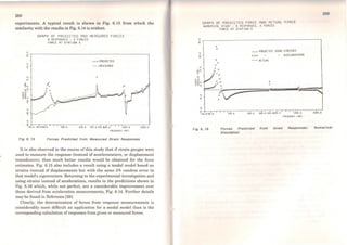
![290
References
(1) Kennedy, C.C., & Pancu, C.D.P. 1947. 'Use of vectors in vibration
measurement and analysis'. J. Aero. Sei., 14(11)
[2) Bishop, R.E.D., & Gladwell, G.M.L. 1963. 'An investigation into the
theory of resonance testing'. Proc. R. Soe. Phil. Trans., 255(A), p. 241
[3) Salter, J.P. 1969. "Steady State Vibration". Kenneth Mason Press
[4) Allemang, R.J. 1984. 'Experimental modal analysis bibliography'.
Proc. IMAC2
[5) Mitchell, L.D., & Mitchell, L.D. 1984. 'Modal analysis bibliography -
An update-1980-1983'. Proc. IMAC2
(6) Ewins, D.J., & Griffin, J. 1981. 'A state-of-the-art assessment of
mobility measurement techniques - Results for the mid-range
structures'. J. Sound & Vib., 78(2), pp. 197-222
[7] Cooley, J.W., & Tukey, J.W. 1965. 'An algorithm for the machine
calculation of complex Fourier series'. Maths. of Comput., 19(90),
pp.297-301
[8) Newland, D.E. 1975. "Random Vibrations and Spectral Analysis".
Longman Press
[9] Bendat & Piersol. 1971. "Random Data: Analysis and Measurement
Procedures". Wiley-lnterscience
[10] International Organisation for Standardisation (ISO). "Methods for
the Experimental Determination of Mechanical Mobility".
Part 1: Basic definitions
Part 2: Measurements using singJe-point translation excitation with
an attached vibration exciter
Part 3: Measurement of rotational mobility
Part 4: Measurement of the complete mobiJity matrix using attached
exciters
:w1
Part 5: Measurements using impact cxcilution with ou t•iu•itt•r· whll'h
is not attached to the structure
[11] White, R.G., & Pinnington, R.J. 1982. 'Praclical applicolio11 of 1ho
rapid frequency sweep technique for structural frcqucncy rt•Hpo11110
measurement'. J. Roy. Aero. Soe.
[12] Halvorsen, W.G., & Brown, D.L. 1977. 'Impulse tochniqW for
structural frequency response testing'. J. Sound & Vib., pp. 8-21
[13] Simon, M., & Tomlinson, G.R. 1984. 'Application of thc Hillwrt
transfonns in the modal analysis of non-linear systoms'. J. So1mcl &
Vib., 96(3)
[14] Gaukroger, D.R., Skingle, C.W., & Heron, K.H. 1973. 'Nunwncol
analysis ofvector response loci'. J. Sound & Vib., 29(3), pp. 341 :Jõ:l
[15] Copley, J.C. 1980. Numerical analysis of vector responscs'. lloynl
Aircraft Establishment Technical Report 80135
[16] Ewins, D.J., & Gleeson, P.T. 1982. 'A method for modal identificai ion
oflightly damped structures'. J. Sound & Vib., 84(1), pp. 57- 79
[17] Brown, D.L., Allemang, R.J., Zimmerman, R., & Mergeay, M. 19W.
'Parameter estimation techniques for modal analysis'. SAE Conirr<'Rll
and Exposition, Detroit
(18] Pappa, R.S., & Ibrahim, S.R. 1981. 'A parametric study of the lbrahim
time domain modal identification algorithm'. Shock & Vib. Bull., 51(:l)
(19] Goyder, H.G.D. 1980. Methods and application ofstructural modolling
from measured structural frequency response data'. J. Sound & V1b.,
68(2), pp. 209-230
(20] Vold, H., Kundrat, J., Rocklin, G.T., & Russell, R. 1982. 'A multi-input
modal estimation algorithm for mini-computers'. SAE Int. Congrcss
and Exposition, Detroit
(21] Berman, A., & Wei, F.S. 1981. 'Automated dynamic analytical modcl
improvement'. NASA Contract Report 3452
[22] Targoff, W.P. 1976. 'Orthogonal check and correction of measured
modes'. AIAA J., 14
(23) Baruch, M. 1980. 'Proportional optimal orthogonalisation ofmeasurcd
modes'. AIAA J., U~7)
[24) Dobson, B.J. 1984. 'Modification of finite element modela using
experimental modal analysis'. Proc. IMAC2
[25] Ewins, D.J., & Sidhu, J. 1984. 'Correlation of finito clcmcnt ond
modal test studies of a practical structure'. Proc. IMAC2](https://image.slidesharecdn.com/133501854-d-j-ewins-modal-testing-theory-and-practice-150524151503-lva1-app6891/85/133501854-d-j-ewins-modal-testing-theory-and-practice-155-320.jpg)
![292
(26] Ewins, D.J., Silva, J.M.M., & Malcci, G. 1980. 'Vibrat.ion analysis of a
helicopter with an externally-att.ached carrier structure'. Shock &
Vib. Bull., 50, Part 2, pp. 155-171
(27) Ghlaim, K.H., & Martin, K.F. 1984. 'Reduced component modes in a
damped system'. Proc. IMAC2
(28) Hillary, B., & Ewins, D.J. 1984. 'The use of strain gauges in force
determination and frequency response function measurements'. Proc.
IMAC2
(29) Zaveri, K. "Modal Analysis of Large Structures - Multiple Exciter
Systems". Bruel and Kjaer Publication
[30) Cawley, P. 1984. 'The reduct.ion of bias error in transfer function
estimates using FFT-based analysers'. Trans. ASME, J. Vib. Ac.
Stress & Rel., 106(1)
..
Notation
This list is extracted from the Notation for Modal Analysis and
Testing, proposcd and adopted in 1993. Also used by the Dynamic Testing
Agency.
1. Basic Terms, Dimensions and Subscripts
X, y, Z
f(t)
t
m
N
n
s
r
j, k, l
p
(1)
translational degrees of freedom/coordinates
(time-varying)
rotational degrees of freedom/coordinates (time-
varying)
timc-varying excit.ation force
timo variable
numbor ofincluded/etrective modes
total numbcr of dcgrecs of frcedom/coordinates
number ofprimary/mastcr/measured DOFs
numbcr of sccondary/slave/unmeasured DOFs
currcnt modo numbor or matrix rank
int.cgcrs
principal/modal coordinate
frcqucncy ofvibration (in rad.s-
1
; Hz)
.J-i
2. Matrices, Vectors and Scalars
( ) mat.rix
( } column vector
( ) singlc elcment (ofmatrix or vector)
t .J diagonal matrix](https://image.slidesharecdn.com/133501854-d-j-ewins-modal-testing-theory-and-practice-150524151503-lva1-app6891/85/133501854-d-j-ewins-modal-testing-theory-and-practice-156-320.jpg)
![['Ll
[ ]21
r r
[ J*; { r; (r
transpose ofa matrix; vector (i.e. row vector)
complex conjugate (Herrnitian) transpose of a
matrix
identity matrix
inverse of a matrix
generaliscd/pseudo inverse ofa matrix
complex conjugate of matrix; vector; single
element
matrices ofleft and right singular vectors
rectangular matrix of singular values ( crj is jth
singular value)
transformation matrix
reduced, expanded matrix
p-norm ofa matrix/vector
value ofa norm/error/perturbation
3. Spatial Model Properties
(M), (K), (C), (D] mass, stiffness, viscous damping,
(hysteretic) damping matrices
analytical/theoretical/predicted/FE
matrix
structural
mass,
[Mx] •...
(õM) =(Mx )- (MA), ...
experimentally derived/test mass, ... matrix
mass, ... error/modification matrix
[
[M)u (M)i2 l.......... .......... ' ...
(MJ21 [MJ22
partitioned mass, ... matrix
4. Modal Properties
(l)r natural frequency ofrth mode (rad.s- 1)
Çr viscous damping ratio of rth mode
11r structural damping loss factor of rth mode
mr modal/effective mass of rth mode
kr modal/effective stiffness ofrth mode
Cr modal/effective viscous dampfng of rth mode
(proportional damping)
Q Qfactor
ô logarithmic decrement
eigenvalue matrix
mode shape/eigenvector matrix
mass-normalised mode shape/eigenvector matrix
rth mode shape/eigenvector
jth element orrth mode shape/eigenvector
['I'] ] eigenvector matrix for viscously
[~1~ r~~j.. damped system
r th mode shape/eigenvector for viscously damped
system
5. Response Properties
(H((I))] Frequency Response Function (FRF) matrix
H jk ((!)) individual FRF element between coordinates j
and k (response at coordinate j due to excitation
at coordinate k)
Response Para.meter
Displacement
Velocity
Acceleration
rAJK =~jr ·~kr
(R)
N
R jk = L rAjk /(!);
r =m+l
Response/Force FRF
Dynarnic Compliance
or Receptance [ex((!)))
Mobility l Y((I)))
Accelerance or
Inertance [A((!))]
modal constant/rcsidue
residual matrix
Force/Response FRF
Dynarnic Stiffness
Mcchanicallmpedance
ApparentJEffective
Mass
high -frequency residual for FRF between j and k,
(H jk ((!)))
Impulse Responsc Function (IRF) matrix
individual IRF elemcnt between coordinates j and
k (response at coordinate j due to excitation at
coordinate k)](https://image.slidesharecdn.com/133501854-d-j-ewins-modal-testing-theory-and-practice-150524151503-lva1-app6891/85/133501854-d-j-ewins-modal-testing-theory-and-practice-157-320.jpg)

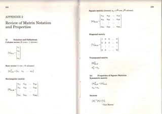
 ~ (B](A)
except for
Symmetry
Symmetric NOT Symmetric
But
Symmetric Symmetric
Also:
and
(iv) Matrix Rank
The product
:101
{<J>}Nxl {<J>}ixN =(A)NxN
<l>~ <l>1 <l>2
where [A] has order N but rank 1.
(v) Pseudo-Inverse
Given equations
we can solve for {y} by:
{Y} =(Ar1 {x}
However, sometimes equations are Overdetermined by redundant data.
Then, we have
where N > M and we cannot solve directly (since (Ar 1
does not exist) so:
from which
(
T )-l T
{y}Mxl = (A) (A) MxM (A)MxN {x}Nxl
or](https://image.slidesharecdn.com/133501854-d-j-ewins-modal-testing-theory-and-practice-150524151503-lva1-app6891/85/133501854-d-j-ewins-modal-testing-theory-and-practice-160-320.jpg)
![302
(Ar is the pseudo-inverse of (A] and gives a least-squares solution of
the redundant equations
303
APPENDIX3
Fourier Analysis
ln this appendix, we list some of the more important features of Fourier
Analysis, as required for most modal testing applications. These will be
summarised in three categories:
(i) Fourier Series
(ii) Fourier Transform
(iii) Discrete Fourier Series (or Transform)
All share the coromon feature of being the means of describing a time-
varying quantity in terms of a set of sinusoids and, conversely, of
reconstituting a time history from a set of frequency components.
Only a summary will be included here. For a more detailed treatment,
refer to a specialist text such as Bendat and Piersol (Reference [9]) or
Newland (Reference [8]). However, it must be noted that there exist slight
differences in definition and terminology which can make cross referencing
from one source to the other somewhat confusing!
(i) Fourier Series
A function x(t) which is periodic in time T can be represented as an
infinite series ofsinusoida:
x(t) = ͪo + °2,(a 0 cosro0 t+ b0 sin ro0 t)
n=l
where](https://image.slidesharecdn.com/133501854-d-j-ewins-modal-testing-theory-and-practice-150524151503-lva1-app6891/85/133501854-d-j-ewins-modal-testing-theory-and-practice-161-320.jpg)
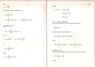


The document discusses modal testing theory and practice, including an overview of applications and measurement techniques, theoretical basis for single and multi-degree-of-freedom systems, and analysis methods to process vibration test data and develop mathematical models of structural dynamics from measurements. Modal testing involves exciting a structure and measuring its vibration response to construct a model of its dynamic properties based on test data rather than theoretical analysis.


![Vibration Fundamentals Training [VFT]](https://cdn.slidesharecdn.com/ss_thumbnails/vftpresentation-130801102551-phpapp01-thumbnail.jpg?width=640&height=640&fit=bounds)


